Comparative analysis of evolving artificial neural network and reinforcement learning in stochastic optimization of multireservoir systems

ABSTRACT

Dynamic programming (DP) has been among the most popular techniques for solving multireservoir problems since the early 1960s. However, DP and DP-based methods suffer from two serious issues: namely, the curses of modelling and dimensionality. Later, reinforcement learning (RL) was introduced to overcome some deficiencies in the traditional DP mainly related to the curse of modelling, but it still encounters the curse of dimensionality in larger systems. Recently, the artificial neural network has emerged as an effective approach to solve stochastic optimization of reservoir systems with high flexibility. In this paper, we develop a single-step evolving artificial neural network (SENN) model that overcomes the curses of modelling and dimensionality in a multireservoir system. Furthermore, a novel efficient allocation technique is developed to ease the allocation of water among different users. A two-reservoir system in Karkheh Basin, Iran, is applied to derive and test the methods. Elitist-mutated particle swarm optimization is used to train the network. A comparison of the results with Q-learning shows the superiority of the SENN, especially during drought periods. Moreover, the SENN performs better in producing more hydropower energy in the system. Thus, the main contributions of this research are (1) development of SENN applications to multireservoir systems, (2) a comparative analysis between SENN and Q-learning especially in prolonged drought conditions and (3) a proposed efficient optimal allocation technique using the simulation method.

Editor D. Koutsoyiannis; Associate editor E. Toth

KEYWORDS:

• Multireservoir system
• evolving artificial neural network
• reinforcement learning
• water allocation
• operating policy
• particle swarm optimization

1 Introduction

Reservoir operation in a basin-wide integrated water resources management (IWRM) scheme is one of the most challenging tasks. This is often due to system complexities and uncertainties. In addition, application of IWRM throughout a river basin with multiple reservoirs can create computational difficulties due to many variables and competing objectives, including the legal contracts and traditions affecting water allocations in a stochastic hydro-meteorological environment (Oliveira and Loucks 1997, Rieker and Labadie 2012). Powerful and adaptive optimization approaches are required to properly handle these issues.

Advances in optimization methods for reservoir operation have been reviewed by several authors including Yeh (1985), Simonovic (1992), Wurbs (1993), Labadie (2004) and Rani and Moreira (2010). These state-of-the-art articles show that simplifications and approximations are required in traditional optimization models for solving real-world reservoir operation problems.

With the advent of metaheuristic algorithms (MAs) as part of the artificial intelligence (AI) techniques, some restrictions inherent in traditional methods including linearity, convexity and derivativity were reduced (e.g. Esat and Hall 1994, Oliveira and Loucks 1997, Wardlaw and Sharif 1999, Kumar and Reddy 2007, Baltar and Fontane 2008, Dariane and Momtahen 2009). Genetic algorithm (GA) (Goldberg 1989, Michalewicz 1996) and particle swarm optimization (PSO) (Kennedy and Eberhart 1995) are among the most popular techniques of MAs with capabilities to solve complex reservoir systems.

Recently, the application of some machine learning techniques such as reinforcement learning (RL) and artificial neural networks (ANNs) in reservoir system operations has drawn attention. RL techniques based on a dynamic programming (DP) framework follow a trial-and-error learning procedure. They are applied to solve Markovian decision problem formulation and thus require a discretized grid over the state-action space, which could lead to dimensionality problems in large-scale systems. To avoid this, some methods such as interpolation, regression, neural networks and fuzzy logic are suggested for value function approximation in RL (Sutton and Barto 1998, Gosavi 2003, Wu 2010, Castelletti et al. 2010). However, these techniques introduce other issues (Gosavi 2003) and may even reduce the system performance. The main advantage of using RL is to overcome “the curse of modelling”, since there is no need to construct the transition probability matrices (TPM) known as the theoretical model of a system (for more details see Gosavi 2003).

The first application of RL in water-related areas was reported by Wilson (1996) for real-time optimal control of hydraulic networks. Later, Bouchart and Chkam (1998) applied RL to a multireservoir operation system in Scotland, where they presented an approach to avoid the curse of dimensionality in RL. In addition, the Q-learning algorithm in RL was first proposed for optimizing the daily operation of a single reservoir system in Italy by Castelletti et al. (2001), and was shown to outperform the implicit stochastic dynamic programming. Lee and Labadie (2007) applied the Q-learning technique for long-term operation of a multipurpose two-reservoir system in South Korea, and then compared it to implicit stochastic dynamic programming and sampling stochastic dynamic programming. The results indicated the superiority of Q-learning over the other two approaches. Other examples of Q-learning applied for water resources systems can be found in Bhattacharya et al. (2003), Mariano-Romero et al. (2007), Mahootchi et al. (2007, 2010), and Rieker and Labadie (2012). Castelletti et al. (2010) applied the fitted Q-iteration combined with tree-based regression to form a suitable function approximator in daily operation of a single reservoir system in Italy. Likewise, a version of multi-objective reinforcement learning was proposed by Castelletti et al. (2013), which is capable of obtaining the Pareto frontier in a single run, and was applied to a single reservoir system operation in Vietnam.

On the other hand, a single step ANN (SENN) model overcomes issues such as the curses of modelling and dimensionality and may thereby be more flexible for solving complex large-scale reservoir system problems. It is worthwhile to mention that the modelling effort in SENN is similar to RL but less than the parametric rule-based metaheuristics. The reason lies in the fact that a complex nonlinear function of operating policy is built implicitly by SENN and RL approaches as opposed to the parametric rule-based metaheuristic models in which a function, often linear, must be defined explicitly and its parameters must be optimized by a metaheuristic. The latter is known as the parameterization–simulation–optimization or parametric method (Koutsoyiannis and Economou 2003). Note that the relationship between state and action variables in reservoir systems is highly nonlinear and, therefore, defining an adaptive and suitable operating policy based on the parametric rule-based metaheuristic models can increase the modelling effort and assumptions about the system.

Common practice to find optimum reservoir operation is through a two-step ANN model coupled with an optimization algorithm. In the first step, the optimization algorithm is used to determine the optimal releases for a long-term period. These optimal actions are then used as the target release patterns to train the ANN model in the second step where if–then operating rules are found. The two-step approach is very similar to the one adopted by Young (1967), in which he used optimal releases by DP to derive reservoir operating rules. Some other similar research has been reported on reservoir systems (e.g. Raman and Chandramouli 1996, Cancelliere et al. 2002, Chandramouli and Deka 2005). In these papers DP was applied to determine optimal actions; however, as mentioned earlier, DP suffers from the dimensionality problem in large systems. Obviously, it is also possible to use MA techniques to obtain optimal actions (e.g. Chang and Chang 2001). However, metaheuristic algorithms also face problems such as low quality of solutions and extremely high computational time when the size of the optimization horizon becomes very long (Dariane and Moradi 2010). Some researchers have applied the observed or simulated operation rules instead of optimal actions derived by DP or MAs (e.g. Wang et al. 2010). However, these target releases may not be optimal and as a result the operation rules obtained by such a method could be suboptimal. Overall, the two-step ANN method suffers from excessive computational time as well as dimensionality issues in the optimization step when applied to large systems with long time horizons regardless of the optimization algorithm used in the process.

Recently, Chaves and Chang (2008) adopted a single-step approach and directly applied ANN to reservoir operation systems. In their approach, ANN is considered as a reservoir controller (the decision maker) applied to control reservoir systems directly. In this approach, unlike the two-step method, ANN does not require optimal target actions. Chaves and Chang (2008) applied this method for the operation of a single reservoir system in Taiwan, using a genetic algorithm (GA) for training the parameters of the ANN model. Also, instead of implementing an allocation model to demand sites, they directly determined water allocation by adding some neuron units to the neural network output layer. Another application of ANN-based control was reported by Pianosi et al. (2011). They coupled ANN with the multi-objective genetic algorithm (NSGA-II) for optimal operation of a single reservoir system in Vietnam.

According to the literature, both applications of single-step ANN-based control were limited to systems with single reservoirs and there seems to be no application for multireservoir systems. It is worthwhile mentioning that the complexity inherent in multireservoir systems has been the focus of many papers in the past. These systems require special attention to the selection of a proper optimization algorithm. In addition, the complications in the system configuration (i.e. reservoir and demand sites and their relative location) could intensify the system complexity. Therefore, an allocation method must be devised to distribute optimum releases from upstream reservoirs and other available water sources in the system among different water users during each time step. On the other hand, the spatial and temporal correlations of reservoir inflows are key factors in multireservoir systems. It is important to know how ANN-based models can cope with the complex stochastic processes of inflows. This paper develops a model and shows the application of a single-step ANN (SENN) approach to multipurpose multireservoir system operation in the Karkheh River basin in southwestern Iran. The results are then compared to those of the Q-learning method in RL, especially in prolonged drought periods. In these periods the system would experience more stresses; therefore, it is important to know how the policies derived by the models would perform under these conditions. Likewise, for training the parameters of the ANN model, the algorithm of elitist-mutated particle swarm optimization (EMPSO) (Kumar and Reddy 2007) is applied. In addition, for allocating water to the demand sites, a novel technique is proposed which is faster and easier than the method applied in WEAP software (WEAP 2011).

2 Intelligent learning techniques

2.1 Reinforcement learning

RL employs the concept of interaction of a learning agent with its environment using the notion of states, actions and rewards (Sutton and Barto 1998). Q-learning as a well-known technique of RL was first introduced by Watkins (1989). It is based on the Q-factor and the Robbins-Monro algorithm. The value function of DP known as the Bellman optimality equation is used for many RL techniques; hence, RL is derived from DP (Gosavi 2003).

The general steps of the Q-learning technique are described as follows. At the beginning of the algorithm one state i from the lookup table is randomly selected (i.e. one storage volume as the state variable at the beginning of period t). The lookup table is the archive of feasible discrete storage (state) and release (action) volumes. Then action a based on an action selection rule, often an ε-greedy rule, is chosen (i.e. one release volume over period t as an action is selected from the lookup table based on a policy of action selection). State j (feasible discrete storage volume at the end of period t) is calculated by simulating the reservoir system. This calculation is performed based on equations related to the reservoir systems (for more details see Section 4.3). The immediate reward function, r(i, a, j), is found by the transition from state i to state j under action a by simulating the system. The immediate cost/reward function is indeed the objective function for measuring the performance of the entire system over period t. The Q-learning relationship defined by the Bellman equation is expressed as follows (Gosavi 2003):

(1)

The above equation illustrates the value function of the Q-learning technique which has the capability of being updated. The indices t and k show operation periods (month, week, day, etc.) and iterations (updates) of the Q-learning function, respectively. The variable α is called the learning rate (step size) and its value is usually equal to , where AA is an assumed value between 0 and 1, and is the number of samples produced in state i and by action a, i.e. the number of times the agent sees state i and action a up to the kth update. The discount rate constant has a positive value less than 1. A(j) implies the set of all feasible discrete actions in state j. Optimal action policy after the kth iteration (i.e. k_max) is obtained as . 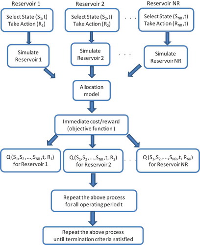This process is repeated until termination criteria are satisfied (e.g. k reaches k_max). The allocation model applied for reservoir systems is described in Section 3. Figure 1 shows the Q-learning modelling technique adapted for multireservoir systems. According to this figure, S and R are respectively the storage and release applied to reservoir systems. Moreover, seasonality index t is used as an additional state variable in order to enhance the results. NR is the total number of reservoirs. Other terms are as defined earlier.

Figure 1. Schematic diagram for Q-learning modelling of multireservoir systems.

As was mentioned earlier, the ε-greedy rule is usually applied to select actions. The ε-greedy action selection employs both greedy and nongreedy rules but with more probability weight on the greedy side. When the nongreedy rule is selected (i.e. taking a random feasible action in state i), then the current knowledge among actions in state i is explored. However, when greedy rule is selected (i.e. selecting the feasible action in state i with the best Q-learning value as ), the current knowledge is exploited. This is a way to balance exploration and exploitation among actions in each state (for more details see Sutton and Barto 1998). An action in state i is selected by ε-greedy as follows:

(2)

where ε is between 0 and 1. If ε is equal to 1 then the ε-greedy becomes greedy. If ε is equal to 0 then the ε-greedy becomes nongreedy.

Likewise, the transition probability matrix (TPM) can be approximated by using a simulator provided that the probability density functions (pdf) of random variables (e.g. reservoir inflow) are determined (Gosavi 2003). In this regard, historical observations can also be applied instead of their pdf (e.g. Lee and Labadie 2007, Castelletti et al. 2010).

2.2 Artificial neural network

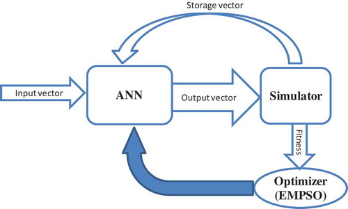
In this research a single-step evolving ANN (SENN) model is developed for optimization of a multipurpose multireservoir system. The basic concept of control processes via ANN-based models is to provide a complex nonlinear relationship between input vector as state variables and output vector as action variable to obtain operating rules without using any target pattern. In this method, the output vector of SENN is adjusted through a reservoir system simulator. The output vector can be either reservoir release or end of period reservoir storage. Here, we used reservoir release as the output of the SENN model. Then simulated variables (e.g. release, storage, evaporation, etc.) are used to evaluate the objective and/or fitness function. Under the proposed procedure the objective function of the SENN model can be the maximization of system performance or the minimization of system losses and costs. It is worthwhile to mention that the back-propagation method is limited to minimizing the sum of error indices. Therefore, unlike the common practice, a training method other than back-propagation must be adopted to handle such objective functions. From this perspective, metaheuristic optimization algorithms can be applied to train the network and find the optimal solution. This process is called the optimizer engine of a system. Figure 2 shows schematically the modelling of a reservoir system using the proposed SENN method and could be applied for single or multiple-reservoir problems.

Figure 2. Schematic diagram for the proposed SENN modelling of reservoir systems.

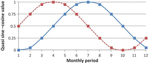
Input vector components (input patterns) can be reservoir storage, inflow, release and also demand in current time t or delayed time t − 1, t − 2, etc. In addition, a pattern of quasi sine–cosine for representing seasonality in the annual cycle (Fig. 3) can also be applied to help the ANN model distinguish among different time periods within the year. It is clear that using a large dimensional input vector would increase the number of synaptic weights of the ANN model and thus could cause computational issues. Therefore, among several components the best ones are chosen by trial and error in order to increase the system performance and decrease the run time.

Figure 3. The seasonality indices (the pattern of quasi sine–cosine).

A feed-forward ANN with one hidden layer can be generally expressed as:

(3)

(4)

where and are the numbers of neurons in the hidden layer and output layer, respectively; and are related to adjustable synaptic weights (connections); and denote the activation functions (using a Log-sigmoid function for the hidden layer and a linear function for the output layer); is input vector; and imply the network outputs of the hidden layer and output layer, respectively; r is the index used to denote each reservoir and NR is the total number of reservoirs.

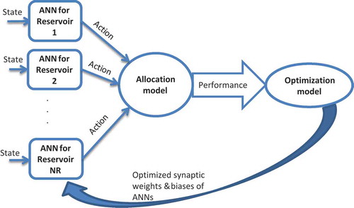
This modelling can be also expressed for multireservoir systems in more detail as shown in Fig. 4. To train the parameters of ANN, a metaheuristic technique must be applied. Therefore, in this research EMPSO is chosen based on the authors’ experience.

Figure 4. A typical SENN approach proposed for multireservoir systems.

2.2.1 Elitist-mutated particle swarm optimization

Particle swarm optimization (PSO) was first introduced by Kennedy and Eberhart (1995). Like many MAs, PSO is based on a solution archive that is often initiated at random. Each solution in the feasible continuous space of the problem is implied as a particle. All particles are stored in an archive called a swarm. The position of each particle i () related to the parameters of ANN (i.e. synaptic weights and biases) is defined by its velocity as follows:

(5)

The velocity of particle i is expressed by the following formula:

(6)

where and are called the constriction coefficient and inertial weight constant, respectively; and are positive acceleration coefficients defined by the user; and are valued by a uniform random number generator to between zero and one; and respectively stand for the best position of particle i and the best position among all particles found up to the current moment.

Kumar and Reddy (2007) proposed the technique of elitist-mutated particle swarm optimization (EMPSO) to overcome the issue of premature convergence in PSO. They applied EMPSO for optimization of a reservoir system operation. The main concept of the EMPSO approach is that the mutation operator acts on the best particles and makes small turbulence among them so that they can discover new positions and overcome getting trapped in local optimal solutions. These new positions are replaced with those of the worst particles. This physical concept can also be shown by the following mathematical formula:

(7)

where, randn is the Gaussian random number with mean 0 and standard deviation 1 known as the standard normal random number; and domain is the parameter’s range in the optimization algorithm. Here, parameters that consist of synaptic weights and biases of the ANN model usually have a range between −1 and 1. Finally, is the ith worst particle that is improved by the mutation operator, as described above.

3 Allocation model

Some researchers have applied LP for allocating water among different demand sites (e.g. Chang et al. 2010). In their procedure LP is used for minimizing water shortages among demand sites within the reservoir system, so that release allocations are part of the system’s decision variables. Application of this procedure introduces many extra decision variables into the problem which may cause dimensionality issues and excessive computer run time. Also, more linearization simplifications are needed for solving a hydropower problem owing to the nonconvexity of the objective function. Another methodology can be used where the reservoir system operation and allocation of releases are dealt with through two separate models. In this approach, the inputs of the allocation model are the optimal releases by the reservoir system at each iteration. This methodology seems to be more flexible and uses fewer decision variables. Water allocation among different users is usually carried out through a presumed general rule. In many cases where equal priority is assumed, the objective is to allocate water by keeping equal percentages of fulfilled demand or deficit among different users, as much as possible. Obviously, when users have different priorities during water shortages, the allocation process becomes simpler by following the water rights. In addition, when some sites are given one priority and others another one, it is clear that demands of sites with priority 1 are met first using the above-mentioned procedure (i.e. same percentage of demand met among elements with the same priority), then the remaining water is used to fulfil demands of sites with priority 2, again following the same procedure for allocating it among different users in this category. Some water resources software such as WEAP (2011) solves the allocation problem using an LP method with an iterative process. The iterative LP method is suitable for simulation programs but it is very time consuming when the procedure is used by a heuristic optimization method that works through a tremendous amount of iterations. Here, for each iteration of the optimization model, the allocation model must complete its own iteration cycle for all allocation sites, causing excessive time consumption for each run of the optimization model. The extent of the problem becomes more evident by noting that one might need up to 20 optimization runs just to evaluate one single alternative of the problem. This is due to the randomness property of the metaheuristic optimization method which is required to run the model several times.

In this paper an allocation method is proposed that considerably reduces the computer time consumption. Although the proposed procedure employs a trial and error method to obtain the optimal values, unlike the WEAP program it does not require any optimization process (i.e. LP). The end result is a considerable reduction in computer time usage by the allocation process as compared to the one using WEAP. The proposed method strives to allocate water to demand sites with priority 1 using the equal percentage rule. Then the remaining water is allocated among those with priority 2, again using the equal percentage rule. The process is repeated until all priorities are fulfilled. A detailed description of the method is presented in the following.

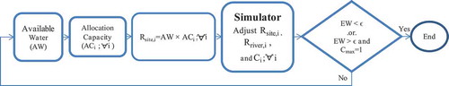
The procedure starts by calculating the available water (AW) and allocation capacity (AC_i) for each site i. AW is the sum of water released from upstream reservoirs and that added by the tributaries in upper sub-basins. AC_i is equal to where D is water demand at site i. Then the flow that must be diverted to each site with the same priority (i.e., i) is determined. This is carried out by multiplying AW and AC_i. Here is a defined value and must be improved by the simulator. As shown by Fig. 5, instream flow demand (R_river,_i) and the actual ratio of supplied demand (C_i) at each site are determined by the simulator. Downstream flow at the end of the system in excess of the minimum instream flow requirement, called the excess water (EW), must be reused if (1) it is greater than ( is a value near zero), and (2) the maximum of parameter C among different sites is less than 1. At the second iteration AW decreases to EW obtained at the previous iteration; and AC_i reduces to . This process is stopped either when EW is less than (i.e. EW) or when EW is significant and greater than but all demands are fulfilled (i.e. EW > and C_max = 1). It is obvious that the value of the actual ratio of supplied demand (C_i) for each site i is limited by 1. As mentioned before, the process presented above is first repeated for the sites with priority 1 and then for the sites with priority 2, and so on.

Figure 5. Proposed allocation technique for complex configurations in multireservoir systems.

Although the result of this approach is exactly the same as those of WEAP software, the computer time consumption by the proposed method is much less. Therefore, the proposed method, which is capable of optimally allocating water to the demand sites without employing any optimization methods, would be very valuable in decreasing computational time, especially for complex and large-scale systems.

4 Case study: Karkheh River basin, Iran

4.1 Overview

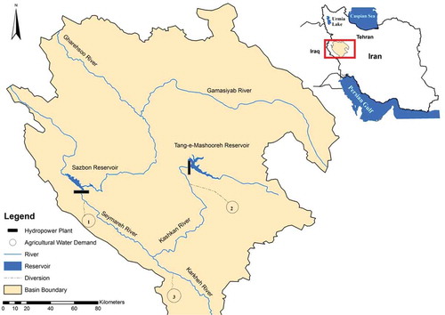
The Karkheh River basin, within geographical coordinates of 46° 23'–49° 12' eastern longitude and 33° 40'–35° 00' northern latitude, is located in southwestern Iran with a basin area of 51 527 km², where 33 674 km² of that is in the highlands and the rest (17 853 km²) is in the plains and foothills. Figure 6 shows the river and reservoir network in the basin. The main Karkheh River is formed by contributions from the Gamasiyab, Gharehsoo, Seymareh and Kashkan rivers. In the eastern part of the basin, the Kashkan River drains a large area of Lorestan province. The Gamasiyab River located in this part of the basin originates from the Malayer and Nahavand plains. In the western part, the Gharehsoo and Gamasiyab join to form the Seymareh River, which flows southward to form the main Karkheh after receiving the Kashkan River. The Karkheh River enters the Hawr-Al-Azim wetland at its end.

Figure 6. Karkheh basin upstream from Karkheh reservoir.

4.2 Data and assumptions

The Sazbon and Tang-e-Mashooreh reservoirs (Fig. 6), which are currently under a feasibility study with the objectives to provide irrigation water for agricultural areas and to produce hydropower energy, are chosen for evaluating the application of the models. For allocating water to users, the proposed allocation technique is incorporated into optimization models. It should be mentioned that the irrigation water demand in this part of the basin is increased by fourfold in order to create stress conditions in the system. Stress conditions make the problem solution more challenging and therefore should be suitable for better model evaluation. Initial storage volumes at each reservoir for both training and testing phases are the same and equal to the average active storage.

The minimum and maximum storage volumes (S_min and S_max) are 957.4 and 1609 million cubic meters (mcm) for Sazbon and 352 and 950 mcm for Tang-e-Mashooreh. The minimum storage for generating hydropower energy (P_min) in the Sazbon and Tang-e-Mashooreh reservoirs is 1132.3 and 352.4 mcm, respectively. In addition to releases from upstream reservoirs, there are also two tributaries in the downstream that help to meet the demands. Agricultural areas 1 and 3 have demands extending from October to April of each year; however, for area 2 the demand period is from April to November. In this research, all three water demand sites have the same priority in receiving water.

The available historical observations include a 47-year period from October 1954 to September 2001, of which the initial 35 years (October 1954 to September 1989) of data are used for training and the last 12 years (October 1989 to September 2001) are employed for testing the trained models. After some investigation, the input layer was determined to include patterns of reservoir inflow, starting reservoir storage, and quasi sine/cosine vectors. The quasi sine/cosine vectors are used to reflect the seasons’ index in the problem. It helps the network to differentiate among seasons within the year by linking each data point with a specific seasonal index. Another approach to model a seasonal problem is either to ignore seasonality links and assume one single time series without any seasonal dependence or to develop one separate model for each season (i.e. 12 models in the case of monthly time steps). Garbrecht (2006) compared several approaches and showed that seasonality differentiation is necessary. Meanwhile, Nilsson et al. (2006) developed a model that included seasonality using two time series representing an annual cycle consisting of quasi sine/cosine vectors. The values of seasonality indices are obtained from Fig. 3.

4.3 Mathematical optimization model formulation

The system considered in this research is a multipurpose optimization problem with the goal of minimizing water demand deficits and reservoir spills as convex functions, while maximizing hydropower energy production as a nonconvex function. These goals are combined into a single objective function with the priority weighting factors in the form of normalized cost functions as follows:

(8)

where T, ND and NR are the number of operation periods, the number of demand sites, and the number of reservoirs in the system; , and are constant weighting coefficients of the objective function based on priority for diversion at site i, hydropower energy production, and reservoir spill, respectively; and are target demand and flow diverted to site i in month t, respectively. The function is the electricity generation at power plant i with the components of and as the average head and turbine discharge during period t, respectively; , and are storage at the beginning and at the end of the period t, respectively; is the installed plant capacity at power plant i and is the number of hours in period t to generate the total energy (firm and secondary); and are spill and the maximum spill at reservoir i over period t. Maximum spill is defined as the difference between reservoir inflow and controlled release. All the objectives are normalized between 0 and 100 in percentage terms to form into a single function. Thus, the goal is to minimize the objective function F. Clearly, the positive signs in the first and last of the three components of the objective function are implemented to minimize the irrigation demand deficits and spillage from reservoirs, respectively. The second term with negative sign is used with the aim of maximizing hydropower energy production. A single objective method is used to handle the problem.

Constraints include the continuity equation and lower and upper bounds on reservoir storage and release. The mass balance equation at reservoir i is:

(9)

where , and are inflow, release and evaporation from reservoir in period t, respectively. Other terms are as defined earlier. It should be mentioned that all the variables in this paper are volumetric and determined in the unit of million cubic metres (mcm), unless otherwise stated.

The reservoir storage and release are subjected to their minimum and maximum bounds as follows:

(10)

(11)

where, R_min,i and are the minimum instream flow requirement and maximum allowable river flow below reservoir i, respectively.

The total generation of electricity includes the firm and secondary energies (in the unit of kilowatt hour, kWh), which are bounded by their upper limits due to plant capacity as follows:

(12)

(13)

where , and are the firm, secondary and total turbine discharge; is the plant efficiency; and is the plant factor over period t at power plant i.

To calculate turbine discharge needed to generate the firm energy, it is first assumed that the energy is equal to its maximum value as:

(14)

If reservoir release is greater than and water level is also above the penstock over period t, then firm energy is generated fully. Otherwise, this amount is reduced to the extent possible. Whenever firm energy is generated fully, secondary energy will be also produced. The production process of secondary energy is similar to that of the firm energy. It is worthwhile to mention that excess reservoir spills can also be utilized to generate firm or secondary electricity.

4.4 System performance measures

Some in-depth performance measures for considering the reliability and vulnerability of the system (Hashimoto et al. 1982, Loucks et al. 2005) are presented as follows:

(15)

(16)

(17)

where is defined as a failure threshold. Its value is in the range of 0 to 1; j and t are year and season indices. In M1, T is the total number of periods considered for computation. Failure threshold is defined as the least percentage of demand that must be met to consider the action a success. All other abbreviations are as defined earlier. In each period, if is less than , then the system has failed and as a result receives 1. Obviously, shows the occurrence of satisfactory performance of the system for site i over period t. The equation for M1 gives the reliability of the system. The system vulnerability is usually defined by the average (M2) and maximum (M3) vulnerabilities as illustrated above.

4.5 Model settings

4.5.1 Q-learning settings

The appropriate setting for the parameters of Q-learning (Section 2.1) for this system were found to be AA = 1, , and . For infeasible policies, a penalty was added to the Q-learning equation (value function). In addition, it was found that a dense state discretization grid may not improve the operating policy while it increases the computational requirements and run time as mentioned by Castelletti et al. (2010), especially for larger dimensional systems. In fact, according to the uncertainties in reservoir operations it seems that using a coarse state discretization grid could lead to the generation of a suitable operating policy with lower computational time consumption. It was also found that applying an efficient discretization grid can improve the quality of operating policy. Therefore, among different values of reservoir storage state discretizations, settings of 15 and 10 grid points for Sazbon and Tang-e-Mashooreh reservoirs, respectively, provided the best policy. The range of storage volume discretizations of Sazbon and Tang-e-Mashooreh reservoirs are from 957.4 to 1609 and 352 to 950 mcm, respectively. Also, among different values of reservoir release discretizations, setting 30 grid points for both reservoirs provided the best policy. Thus, releases of both reservoirs were discretized assuming 10 points for the range [0–R_min,_i] and 20 points for the range [R_min,_i–R_max,_i] for each month. In Q-learning, two different models were developed. Model 1 uses storage as the only state variable. In model 2, seasonality was added as another state variable. Two cases were also defined that are different in the number of Q-learning equation (function evaluation) updates. In case 1, the number of function evaluations is the same as that of case 1 of SENN (see the next subsection). However, in case 2 the number of Q-learning function updates was set equal to 4 000 000. The actions, which are assumed to be reservoir releases in all Q-learning models, are taken by applying the ε-greedy policy. Moreover, the solutions are evaluated based on the results obtained through 10 independent runs for each model scenario, due to the randomness of the technique.

4.5.2 SENN settings

Suitable values for EMPSO parameters (Section 2.2.1) were determined through a trial and error process. They were found to be , = 0.9 and , with the size of swarm equal to 100. In addition, the number of iterations before the mutation process, the number of particles to be elitist-mutated and the probability of mutation were chosen as 50, 0.05 per cent of the size of swarm (0.05 ) and 0.03, respectively, based on previous experience.

Furthermore, it was noticed that the training process of the SENN model can be categorized into two different cases. The distinction is mainly based on including or excluding a validation period in the training process. As we know, in the normal training process of any ANN model a validation period is used to determine the stopping epoch in order to avoid overfitting by the model. As we will discuss later in Section 4.6, the possibility of an overfitting by the ANN model is very small when trained by a heuristic method (Sexton et al. 1998). Therefore, it is possible to omit the validation period and combine it into the training period to take advantage of longer calibration datasets. In case 1, the regular method of using a validation period is employed where the data for the first 28 years are used for training and the next 7 years are set for validation. However, in case 2 the validation period is removed and data for the whole 35 years are included for training the model. The last 12 years of data in both cases are used to test the model.

The stopping condition for case 1 in the SENN model is when the objective function does not improve using the validation data after 300 iterations. For a better comparison, case 2 is evaluated using two different numbers of function evaluations. In case 2a the number of function evaluations of each model is the same as that of case 1. However, in case 2b it is assumed to be a large number of function evaluations (4 000 000). To further demonstrate the impact of different inputs on the model performance, a stepwise method was adopted. Accordingly, four different model alternatives were developed in cases 1 and 2(a, b) that vary only in input variables (Table 1). Model 1 uses reservoir storage as the only input. In model 2, reservoir inflow is also added to the input. In model 3, reservoir storage and seasonality indices are the model inputs. Finally, model 4 includes reservoir storage, inflow and seasonality indices as the input matrix. Similarly to Q-learning, the action variable in each SENN model is assumed to be the reservoir release.

Table 1. Comparison of testing period results of SENN models: 10 runs.

Evaluation criterion	Objective function
	Case 1				Case 2a using number of function evaluations as Case1				Case 2b using large number of function evaluations
	1	2	3	4	1	2	3	4	1	2	3	4
State variables:	S	S, I	S, t1, t2	S, I, t1, t2	S	S, I	S, t1, t2	S, I, t1, t2	S	S, I	S, t1, t2	S, I, t1, t2
Best	−9.63	−11.08	−12.98	−14.47	−9.67	−11.18	−12.95	−14.53	−9.71	−11.18	−13.60	−15.51
Worst	−8.74	−9.11	−11.38	−13.05	−9.32	−10.70	−12.30	−13.15	−9.40	−10.70	−12.57	−14.17
Mean	−9.31	−10.51	−12.53	−13.78	−9.53	−10.96	−12.67	−13.80	−9.59	−10.88	−13.12	−14.84
St. dev.	0.345	0.61	0.47	0.46	0.13	0.16	0.19	0.43	0.11	0.15	0.37	0.38
Mean number of function evaluations	42 400	46 300	100 400	158 800	424 000	46 300	100 400	158 800	4 000 000

Using a trial and error method, it was found that a set of four neurons in the hidden layer is suitable for all ANN models. The initial values of synaptic weights and biases were randomly selected in the range [−1, 1]. Moreover, this range was then developed to [−10, 10] for better performance and more flexibility in finding optimal solutions. The minimum and maximum velocities for the particles (V_min and V_max) were set to −100 and 100, respectively. The initial value of velocity for all particles was also set to zero. As was mentioned earlier, the input layer for the ANN model includes patterns of reservoir inflow, starting reservoir storage and seasonality index. The output vector is the reservoir release during the current period. Similarly to the Q-learning, 10 independent runs are carried out for each SENN model.

4.6 Results of SENN in different set-ups

Table 1 shows the results of SENN models in different set-ups. A unique objective function is used by all models as described earlier. It is clear from Table 1 that, in all cases, model 1 cannot achieve an acceptable reservoir operation policy. The result of model 2 reveals that the reservoir inflow is an effective signal to improve the operation policy. Comparing the results of models 1 and 3, and models 2 and 4, indicates the importance of seasonality index in these models. It can be seen that the seasonality indices can improve the objective function value more than the reservoir inflow does. For example, a comparison of models 1, 2 and 3, again in all cases, shows that on average the inclusion of seasonality indices beside the reservoir storage improves the objective function by more than 3 units, while improvement when inflow is added is barely over 1 unit.

A comparison of results by the SENN model in cases 1 and 2(a, b) shows that when validation is removed and more data are used by the training process, the overall performance of the model is improved. It can also be concluded that, as expected, using a higher number of function evaluations (case 2b) helps to further improve the results. By comparing the results, model 2b.4 (case 2b model 4) is chosen for further analysis.

Overfitting is known as an important issue in most data-driven methods, including the artificial neural networks, and proper precautions must be used to avoid it. A review of results indicates that since performances improve over the test set in cases 2a and 2b, overfitting does not occur in this application. Among other factors, the training method of ANN can have an important role in preventing the overfitting (Pendharkar 2007). On the other hand, Sexton et al. (1998) indicate that overfitting in ANNs trained by evolutionary algorithms is not a serious problem as opposed to ANNs trained by back-propagation techniques. Moreover, since evolutionary algorithms are search-based techniques, they obtain solutions via generating the random numbers to reach global optimum, and most of them work with an archive of potential solutions. These inherent properties cause the diversity between the solutions, helping ANN to learn the general patterns (Pendharkar and Rodger 2004), and not fitting each point including noise and error. Therefore, they can find the true underlying function. Thus we can conclude that, in order to improve the results in evolutionary ANN, the validation period can be omitted and the datasets can be included for training the model.

4.7 Comparative analysis of SENN and Q-learning

As mentioned earlier, in Q-learning two different model alternatives were applied which vary only in input variables (Table 2). Model 1 uses reservoir storage as the only input. In model 2, seasonality was added as another state variable. The actions are taken by applying the ε-greedy policy. As can be seen from Table 2, similarly to the SENN method, the inclusion of seasonality beside the reservoir storage improves the results of the Q-learning model.

Table 2. Comparison of testing period results of Q-learning models: 10 runs.

Evaluation criterion	Objective function: Q-learning
	Case 1		Case 2
	1	2	1	2
State variables	Storage	Storage and seasonality	Storage	Storage and seasonality
Best	−8.72	−11.42	−9.25	−12.46
Worst	−6.80	−10.85	−6.80	−11.73
Mean	−8.05	−11.12	−8.22	−12.07
St. dev.	0.61	0.18	0.82	0.24
Number of function evaluations as SENN	42 400	100 400	4 000 000

Note: Case 1 and Case 2 respectively, equivalent to case 2a and 2b of SENN in Table 1.

A comparison of results indicates that overall the performance of SENN is better than that of Q-learning using either a single (i.e. storage) or multiple state variables (i.e. storage and seasonality). However, it is not possible to conclude the superiority of SENN over Q-learning when more state variables (such as inflow) are added. Nevertheless, the overall evaluation of the two methods should not only be based on the value of objective function but other criteria such as the computational burden must also be considered. Therefore, it is not possible to conclude the superiority of SENN over Q-learning when more state variables (such as inflow) are added.

Further comparison shows that the standard deviation (st. dev.) of 10 runs by SENN is relatively better than Q-learning when only the storage is used. However, Q-learning shows lower standard deviations when both storage and seasonality are used as state variables. Moreover, since SENN can handle as many input variables as necessary with the lowest computational cost within a reasonable run time, it is possible to add more state variables to improve the results. It is also possible to include more input state variables in Q-learning; however, the computational burden would be high.

The final results derived by SENN and Q-learning as well as the perfect solution are presented in Table 3. The input matrix in SENN includes seasonality, reservoir inflow and storage volume as state variables; whereas, in Q-learning the storage volume and seasonality are the state variables. In the perfect model, the problem is solved using the EMPSO algorithm under perfect foreknowledge of the 12-year testing period without any predetermined operating policy. The results of the perfect model can be considered as an upper bound of the solutions by other methods, since unlike the SENN or Q-learning the perfect model is not constrained by any operation policy. In fact, in the perfect model the optimization algorithm finds the optimum route for the testing period assuming that all inflows and demands are known beforehand. However, the result may be different from the global solution since there is no assurance that any heuristic method will reach the global optimum solution. According to research by Moradi and Dariane (2009) for similar problems, the EMPSO is capable of reaching near global optimum solutions.

Table 3. Summary of objective functions found by the models: 10 runs.

Method	SENN	Q-learning	Perfect model
Best	−15.51	−12.46	−18.13
Worst	−14.17	−11.73
Mean	−14.84	−12.07
St. dev.	0.38	0.24

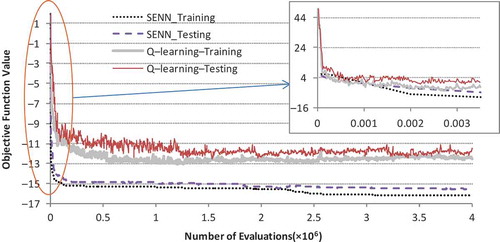
Figure 7 shows that the SENN model has a better convergence toward the optimal solution than the Q-learning. It shows that the SENN model starts faster convergence in the early iterations. To improve the convergence speed of the Q-learning model, metaheuristic methods can be incorporated into that model (see, e.g. Iima and Kuroe 2008, Iima et al. 2010). In addition, the results obtained by the SENN are closer to the solution by the perfect model.

Figure 7. Comparison of solution convergence by SENN and Q-learning.

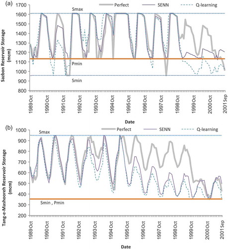
The results for the Sazbon reservoir, as shown in Fig. 8, indicate that over the prolonged drought period from October 1998 to September 2001, unlike the Q-learning method, the SENN model was able to keep the reservoir storage from falling under the penstock level (P_min). A similar trend is observed for the Tang-e-Mashooreh reservoir (Fig. 8(b)) where the P_min and S_min are nearly the same. In both reservoirs, the storage levels obtained by the SENN are higher than those of Q-learning. As can be seen from Fig. 8(a), in some periods the perfect model allows the Sazbon reservoir level to fall under P_min. This is normal due to the fact that the perfect model optimizes the operation of the system for the whole 12-year period using predetermined inflows. In other words, it has knowledge about the inflows of the whole 12-year period when making decisions on releasing water in year 1. Other models also use deterministic information, but their optimal decision variables are determined during an earlier training stage using different information. SENN and Q-learning follow an offline approach during the testing period and are no longer able to adjust the decision parameters of their operating policy using the current information.

Figure 8. Comparison of reservoir storage during the testing period for (a) Sazbon and (b) Tang-e-Mashooreh reservoirs.

The proposed SENN method provides the advantage that it can easily be scaled to use a higher quantity of input information, which is the key factor in improving the operation performance. On the other hand, although in principle Q-learning may also include more input information, in practice it is severely limited by the increase in computing time and dimensional problems generated by any new state variable, especially when it is applied for large-scale systems. It is worth mentioning that the policy derived by Q-learning can likely be improved by revising the performance function (Lee and Labadie 2007) or using a hedging rule so that it could be suitable for droughts. Also, using a suitable discretization grid over the state-action space can improve the operating rules (Castelletti et al. 2010).

Although not shown here, a comparison of firm energy production by the three models in the Sazbon reservoir made it clear that while SENN is very close to the perfect model, Q-learning fails to produce the required firm energy in most periods of the drought years.

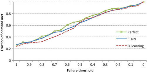
In general, as can be seen from Fig. 9, the SENN model has been able to increase the reliability (M1) and decrease the vulnerability (M2, M3) of the system. In deriving these figures, a failure is assumed to occur whenever the quantity of water provided to a site is less than its target demand during each time step (i.e. as discussed earlier in Section 4.4). As a further analysis, several threshold levels for demand are assumed and their corresponding reliabilities are estimated following different models. Figure 10 compares the results of such analysis. Once again, as can be seen from Figure 10, the SENN outperforms Q-learning and is close to the perfect model.

Figure 9. Comparison of performance measures (M1, M2 and M3 denote reliability, and average and maximum vulnerability of the system, respectively).

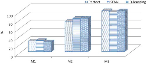
Figure 10. Reliability with several failure thresholds.

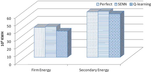
It is interesting to note that, as Figure 11 shows, overall the firm and secondary energy production by the SENN model is higher than those of Q-learning and even the perfect model. It can be seen that optimal operating rules derived by SENN allow increasing total hydropower generation up to 10% by increasing water supply for water users in comparison to Q-learning. Perhaps a question may be raised as to why the perfect model has not provided the best result in energy production. It is clear that the problem is solved in a multiple-objective environment and the solution found by the perfect model for all the objectives must be the best. However, there might be inconsistencies in reaching the best solutions for each objective. In fact, each model performs a trade-off among different objectives and tries to optimize the whole objective function and not necessarily each single one.

Figure 11. Long-term mean monthly hydropower energy generation.

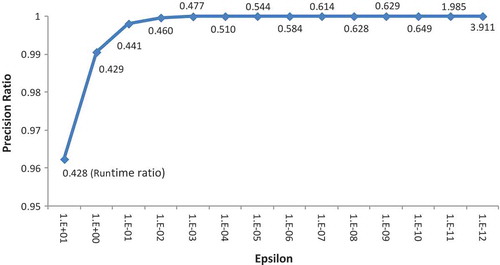
A comparison of the allocations obtained by the proposed allocation technique and the LP method based on the WEAP procedure show that they perform similarly. However, as was mentioned earlier, the main advantage of the new allocation approach is the noticeable reduction in the computational time. Figure 12 shows the results of precision ratio and computational time ratio derived by the proposed allocation technique in comparison with the LP-based (WEAP) method. By the precision ratio we mean the ratio of the optimal solution obtained by the proposed method to that of the LP method. Also, the computational time ratio (numbers next to the curve in Fig. 12) indicates the ratio of time consumption by the proposed method to that of the LP (WEAP). It can be seen that by reducing the value of epsilon (, the parameter of allocation precision, see Section 3) the allocation precision ratio increases; however, the computational time increases accordingly. The results of the two methods nearly become the same when the epsilon value reaches 0.001. At this level the proposed method uses about 48% (nearly half) of the time used by LP. The proposed allocation method outperforms the LP in time consumption for epsilons up to about 1E-10. After that, the proposed method uses more time than the LP method. However, it is not necessary to decrease the value of epsilon that far. In fact, a value of = 0.1, where the time consumption by the proposed allocation method is 44% of that by the LP method, would be suitable for the required precision.

Figure 12. A sensitivity analysis of epsilon parameter with regard to precision ratio (the ratio of the optimal solution obtained by the proposed method to that of the LP-based one) and run time ratio (the ratio of time consumption by the proposed method to that of the LP in WEAP).

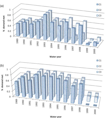
As a further analysis, an example of the actual ratio of supplied demand in each site C_i (see Fig. 3) for October (a period with relatively low inflow and high demand) during the testing phase using Q-learning and SENN models is given in Fig. 13(a) and (b), respectively. It can be seen that the SENN has been able to satisfy the target demands better than Q-learning, especially over the drought years of 1999 and 2000. In addition, the results of Q-learning show that the demand fulfilment ratios for area 2 (C₂) are very low during the dry period of 1996 to 2000. However, the SENN model has been able to avoid such a problem through exploring more enhanced operation rules.

Figure 13. Comparison of October allocations using (a) Q-learning model and (b) SENN model.

5 Summary and conclusions

Stochastic optimization in integrated basin-wide water resources systems is one of the major technical challenges. Although some stochastic techniques based on dynamic programming have been developed in the past, they have all suffered from serious problems including the curse of modelling and the curse of dimensionality so that they cannot be applied to large-scale multireservoir systems. It has also been revealed that reinforcement learning techniques can overcome some problems of traditional methods; however, they are still plagued by the curse of dimensionality in larger problems. Lately, artificial neural networks have been presented to solve stochastic optimization of reservoir systems so that they can solve large-scale systems without any simplification and approximation. ANNs are capable of overcoming the two major issues of the curse of dimensionality and the curse of modelling if a single-step approach is adopted. In this paper a single-step approach was used to develop an ANN model (SENN) for long-term optimum operation of a multipurpose multireservoir system. For this purpose, the algorithm of elitist-mutated particle swarm optimization (EMPSO) was applied to train the ANN model developed for a multipurpose two-reservoir system. The results were then compared to those of Q-learning as a reinforcement learning technique. The models were evaluated using 47 years of data from a two-reservoir system in the Karkheh River basin located in southwestern Iran.

It was found that the SENN model outperformed Q-learning both when the storage was used as the state variable and when seasonality was added. The performance of SENN improved further when inflow (I) was added to the state variables of the model.

The proposed SENN method provides the advantage that it can easily be scaled to use a higher quantity of input information, which is the key factor in improving the operation performance. On the other hand, although in principle Q-learning may also include more input information, in practice it is severely limited by the increase in computing time and dimensional problems generated by any new state variable, especially when it is applied for large-scale systems.

Overall, the results of the SENN model are better than those of Q-learning for the state variables (storage and seasonality) tested in this research and are very close to those of the perfect model. However, it is not possible to conclude the superiority of SENN over Q-learning for cases where more state variables (such as inflow) are considered. The SENN model was able to meet the irrigation demand with higher reliability and lower vulnerability as compared to Q-learning. Moreover, it was able to produce more firm and secondary hydropower energy than Q-learning. The operation rule derived by the SENN demonstrated high performance, specifically during the drought periods.

In addition, a fast allocation method was introduced and compared to the LP method of WEAP to overcome the heavy time consumption problem of the LP. It was found that the proposed allocation method can reach the same solution as the LP in a much shorter time. The proposed method was found to be about 2.3 times faster than LP.

Disclosure statement

No potential conflict of interest was reported by the authors.

References

- Baltar, A.M. and Fontane, D.G., 2008. Use of multiobjective particle swarm optimization in water resources management. Journal of Water Resources Planning and Management, 134 (3), 257–265. doi:10.1061/(ASCE)0733-9496(2008)134:3(257)
- Bhattacharya, B., Lobbrecht, A., and Solomatine, D., 2003. Neural networks and reinforcement learning in control of water systems. Journal of Water Resources Planning and Management, 129 (6), 458–465. doi:10.1061/(ASCE)0733-9496(2003)129:6(458)
- Bouchart, F.-C. and Chkam, H., 1998. A reinforcement learning model for the operation of conjunctive use schemes. In: International conference on hydraulic engineering software, September 1998. Southampton, ROYAUME-UNI: Computational Mechanics Publications, 319–329.
- Cancelliere, A., et al., 2002. A neural networks approach for deriving irrigation reservoir operating rules. Water Resources Management, 16 (1), 71–88. doi:10.1023/A:1015563820136
- Castelletti, A., et al., 2001. A reinforcement learning approach for the operational management of a water system. In: Modeling and Control in Environmental Issues, 22–23 August 2001 Yokohama, Japan.
- Castelletti, A., et al., 2010. Tree-based reinforcement learning for optimal water reservoir operation. Water Resources Research, 46 (9), W09507. doi:10.1029/2009WR008898
- Castelletti, A., Pianosi, F., and Restelli, M., 2013. A multiobjective reinforcement learning approach to water resources systems operation: Pareto frontier approximation in a single run. Water Resources Research, 49 (6), 3476–3486. doi:10.1002/wrcr.20295
- Chandramouli, V. and Deka, P., 2005. Neural network based decision support model for optimal reservoir operation. Water Resources Management, 19 (4), 447–464. doi:10.1007/s11269-005-3276-2
- Chang, L.C. and Chang, F.J., 2001. Intelligent control for modelling of real‐time reservoir operation. Hydrological Processes, 15 (9), 1621–1634. doi:10.1002/hyp.226
- Chang, L.-C., Ho, -C.-C., and Chen, Y.-W., 2010. Applying multiobjective genetic algorithm to analyze the conflict among different water use sectors during drought period. Journal of Water Resources Planning and Management, 136 (5), 539–546. doi:10.1061/(ASCE)WR.1943-5452.0000069
- Chaves, P. and Chang, F.-J., 2008. Intelligent reservoir operation system based on evolving artificial neural networks. Advances in Water Resources, 31 (6), 926–936. doi:10.1016/j.advwatres.2008.03.002
- Dariane, A.B. and Moradi, A.M., 2010. Application of ant-colony-based algorithms to multi-reservoir water resources problems. Journal of Water and Wastewater, 76, 81–91, (In Farsi language).
- Dariane, A.B. and Momtahen, S., 2009. Optimization of multireservoir systems operation using modified direct search genetic algorithm. Journal of Water Resources Planning and Management, 135 (3), 141–148. doi:10.1061/(ASCE)0733-9496(2009)135:3(141)
- Esat, V. and Hall, M., 1994. Water resources system optimization using genetic algorithms. In: Proceedings of the first International Conference on Hydroinformatics. Balkema, Rotterdam, The Netherlands, 225–232.
- Garbrecht, J.D., 2006. Comparison of three alternative ANN designs for monthly rainfall-runoff simulation. Journal of Hydrologic Engineering, 11 (5), 502–505. doi:10.1061/(ASCE)1084-0699(2006)11:5(502)
- Goldberg, D.E., 1989. Genetic algorithms in search, optimization, and machine learning. Menlo Park: Addison-wesley Reading.
- Moradi, A.M. and Dariane, A.B., 2009. Particle swarm optimization: application to reservoir operation problems. In: Advance computing conference, 6 March 2009, Patiala. IEEE International, 1048–1051.
- Gosavi, A., 2003. Simulation-based optimization: parametric optimization techniques and reinforcement learning. Boston, MA, US: Kluwer Academic Press.
- Hashimoto, T., Stedinger, J.R., and Loucks, D.P., 1982. Reliability, resiliency, and vulnerability criteria for water resource system performance evaluation. Water Resources Research, 18 (1), 14–20. doi:10.1029/WR018i001p00014
- Iima, H. and Kuroe, Y., 2008. Swarm reinforcement learning algorithms based on particle swarm optimization. In: International Conference on Systems, Man, and Cybernetics (SMC), 12–15 October 2008. Singapore: IEEE, 1110–1115.
- Iima, H., Kuroe, Y., and Matsuda, S., 2010. Swarm reinforcement learning method based on ant colony optimization. In: IEEE International Conference on Systems, Man, and Cybernetics (SMC), 10–13 October 2010. Istanbul: IEEE, 1726–1733.
- Kennedy, J. and Eberhart, R., 1995. Particle swarm optimization. In: Conference on Neural Networks. IEEE, 1942–1948.
- Koutsoyiannis, D. and Economou, A., 2003. Evaluation of the parameterization-simulation-optimization approach for the control of reservoir systems. Water Resources Research, 39, 6. doi:10.1029/2003WR002148
- Kumar, D.N. and Reddy, M.J., 2007. Multipurpose reservoir operation using particle swarm optimization. Journal of Water Resources Planning and Management, 133 (3), 192–201. doi:10.1061/(ASCE)0733-9496(2007)133:3(192)
- Labadie, J.W., 2004. Optimal operation of multireservoir systems: State-of-the-art review. Journal of Water Resources Planning and Management, 130 (2), 93–111. doi:10.1061/(ASCE)0733-9496(2004)130:2(93)
- Lee, J.-H. and Labadie, J.W., 2007. Stochastic optimization of multireservoir systems via reinforcement learning. Water Resources Research, 43 (11), W11408. doi:10.1029/2006WR005627
- Loucks, D.P., et al., 2005. Water resources systems planning and management: an introduction to methods, models and applications. Paris: UNESCO.
- Mahootchi, M., Ponnambalam, K., and Tizhoosh, H., 2010. Comparison of risk-based optimization models for reservoir management. Canadian Journal of Civil Engineering, 37 (1), 112–124. doi:10.1139/L09-165
- Mahootchi, M., Tizhoosh, H., and Ponnambalam, K., 2007. Opposition-based reinforcement learning in the management of water resources. In: International Symposium on Approximate Dynamic Programming and Reinforcement Learning (ADPRL), 1–5 April 2007. Honolulu, HI: IEEE, 217–224.
- Mariano-Romero, C.E., Alcocer-Yamanaka, V.H., and Morales, E.F., 2007. Multi-objective optimization of water-using systems. European Journal of Operational Research, 181 (3), 1691–1707. doi:10.1016/j.ejor.2006.08.007
- Michalewicz, Z., 1996. Genetic algorithms+ data structures= evolution programs. Berlin: Springer.
- Moradi, A.M., and Dariane, A.B., 2009. Particle swarm optimization: application to reservoir operation problems. In: IEEE international conference on advance computing, 6–7 March, Patiala, 1048–1051.
- Nilsson, P., Uvo, C.B., and Berndtsson, R., 2006. Monthly runoff simulation: Comparing and combining conceptual and neural network models. Journal of Hydrology, 321 (1), 344–363. doi:10.1016/j.jhydrol.2005.08.007
- Oliveira, R. and Loucks, D.P., 1997. Operating rules for multireservoir systems. Water Resources Research, 33 (4), 839–852. doi:10.1029/96WR03745
- Pendharkar, P.C., 2007. A comparison of gradient ascent, gradient descent and genetic algorithm based artificial neural networks for the binary classification problem. Expert Systems, 24 (2), 65–86. doi:10.1111/j.1468-0394.2007.00421.x
- Pendharkar, P.C. and Rodger, J.A., 2004. An empirical study of impact of crossover operators on the performance of non-binary genetic algorithm based neural approaches for classification. Computers & Operations Research, 31 (4), 481–498. doi:10.1016/S0305-0548(02)00229-0
- Pianosi, F., Thi, X.Q., and Soncini-Sessa, R., 2011. Artificial neural networks and multi objective genetic algorithms for water resources management: an application to the HoaBinh reservoir in Vietnam. In: Proceedings of the 18th IFAC World Congress, 28 August– 2 September 2011. Milan, Italy: International Federation of Automatic Control (IFAC), 10579–10584.
- Raman, H. and Chandramouli, V., 1996. Deriving a general operating policy for reservoirs using neural network. Journal of Water Resources Planning and Management, 122 (5), 342–347. doi:10.1061/(ASCE)0733-9496(1996)122:5(342)
- Rani, D. and Moreira, M.M., 2010. Simulation–optimization modeling: a survey and potential application in reservoir systems operation. Water Resources Management, 24 (6), 1107–1138. doi:10.1007/s11269-009-9488-0
- Rieker, J.D. and Labadie, J.W., 2012. An intelligent agent for optimal river-reservoir system management. Water Resources Research, 48 (9), W09550. doi:10.1029/2012WR011958
- Sexton, R.S., Dorsey, R.E., and Johnson, J.D., 1998. Toward global optimization of neural networks: a comparison of the genetic algorithm and backpropagation. Decision Support Systems, 22 (2), 171–185. doi:10.1016/S0167-9236(97)00040-7
- Simonovic, S.P., 1992. Reservoir systems analysis: closing gap between theory and practice. Journal of Water Resources Planning and Management, 118 (3), 262–280. doi:10.1061/(ASCE)0733-9496(1992)118:3(262)
- Sutton, R.S. and Barto, A.G., 1998. Reinforcement learning: an introduction. Cambridge, MA, US: MIT Press.
- Wang, Y.-M., Chang, J.-X., and Huang, Q., 2010. Simulation with RBF neural network model for reservoir operation rules. Water Resources Management, 24 (11), 2597–2610. doi:10.1007/s11269-009-9569-0
- Wardlaw, R. and Sharif, M., 1999. Evaluation of genetic algorithms for optimal reservoir system operation. Journal of Water Resources Planning and Management, 125 (1), 25–33. doi:10.1061/(ASCE)0733-9496(1999)125:1(25)
- Watkins, C.J.C.H., 1989. Learning from delayed rewards. Thesis (PhD). Cambridge University.
- WEAP, 2011. Water evaluation and planning system–user guide. Somerville, MA, US: Stockholm Environment Institute (SEI).
- Wilson, G., 1996. Reinforcement learning: A new technique for the real-time optimal control of hydraulic networks. In: Hydroinformatics Conference. Taylor and Francis, 893–900.
- Wu, C., 2010. Novel function approximation techniques for large-scale reinforcement learning. Thesis (PhD). Northeastern University.
- Wurbs, R.A., 1993. Reservoir-system simulation and optimization models. Journal of Water Resources Planning and Management, 119 (4), 455–472. doi:10.1061/(ASCE)0733-9496(1993)119:4(455)
- Yeh, W.W.G., 1985. Reservoir management and operations models: a state of the art review. Water Resources Research, 21 (12), 1797–1818. doi:10.1029/WR021i012p01797
- Young, G.K., 1967. Finding reservoir operating rules. In: Proceedings of the American Society of Civil Engineers, 297–321.