New fuzzy neural network–Markov model and application in mid- to long-term runoff forecast

ABSTRACT

In this paper, a mid- to long-term runoff forecast model is developed using an ideal point fuzzy neural network–Markov (NFNN-MKV) hybrid algorithm to improve the forecasting precision. Combining the advantages of the new fuzzy neural network and the Markov prediction model, this model can solve the problem of stationary or volatile strong random processes. Defined error statistics algorithms are used to evaluate the performance of models. A runoff prediction for the Si Quan Reservoir is made by utilizing the modelling method and the historical runoff data, with a comprehensive consideration of various runoff-impacting factors such as rainfall. Compared with the traditional fuzzy neural networks and Markov prediction models, the results show that the NFNN-MKV hybrid algorithm has good performance in faster convergence, better forecasting accuracy and significant improvement of neural network generalization. The absolute percentage error of the NFNN-MKV hybrid algorithm is less than 7.0%, MSE is less than 3.9, and qualification rate reaches 100%. For further comparison of the proposed model, the NFNN-MKV model is employed to estimate (training and testing for 120-month-ahead prediction) and predict river discharge for 156 months at Weijiabao on the Weihe River in China. Comparisons among the results of the NFNN-MKV model, the WNN model and the SVR model indicate that the NFNN-MKV model is able to significantly increase prediction accuracy.

Editor D. Koutsoyiannis; Associate editor Y. Gyasi-Agyei

KEYWORDS:

• mid- to long-term runoff
• NFNN-MKV hybrid algorithm
• Si Quan Reservoir
• Weijiabao

1 Introduction

Mid- to long-term runoff forecasting is important for the study and guidance of water resources management. However, accurate forecasts are difficult because hydrological signals are nonlinear, highly complex and have severe variations in time and space (Yang et al. 2013). At present, the research in mid- to long-term runoff prediction is still in the development stage. A variety of mid- to long-term runoff forecasting models have been developed based on physical considerations or other numerical theories, such as Markov prediction models (Wang et al. 2005) based on Markov chain theory; linear regressive analysis methods and nonlinear regressive analysis methods (Shamseldin et al. 1997) based on stochastic theory; SVM (support vector machine) models (Lin et al. 2006) based on nonlinear time series analysis; fuzzy prediction models (Nayak et al. 2004) based on fuzzy theory; and ANN (artificial neural network) models (Dibike and Solomatine 2001) based on black-box theory. However, because of some inaccurate initial conditions and limited parameterization schemes, those models are generally insufficient for making accurate predictions (Gardner et al. 2009, Shi 2010b).

It is a hot issue for scholars all over the world to improve the accuracy of mid- to long-term runoff prediction. A variety of methods have been developed to improve the accuracy of the predictions, including physical models, time series methods, conceptual models, ANN models, and many hybrid models. Now, models integrating two or more of these approaches have been proposed as predictors to improve the accuracy of mid- to long-term runoff forecasts, such as multiple regression–ANN models (Elshorbagy et al. 2000), fuzzy pattern recognition models (Xiong et al. 2001), the wavelet–ANN model (Anctil and Tape 2004, Adamowski et al. 2012, Wei et al. 2012), the wavelet–ANFIS hybrid model (Moosavi et al. 2013, Nourani et al. 2013), the wavelet–neuron fuzzy model (Partal and Kişi 2007, Shiri and Kisi 2010), the fuzzy–SVM model (Guo et al. 2010, Hu et al. 2012), the support vector regression (SVR) model (Lin et al. 2006, Hong and Pai 2007, Wu et al. 2008, Behzad et al. 2009) and the wavelet regression model (Kişi 2009, 2010, 2011). These hybrid models have shown different advantages for accurate predictions due to their capabilities in utilizing present information effectively. Among these hybrid models, FNN (fuzzy neural network) and ANN models are the most popularly utilized sub-models for signal forecasting due to their capability of effectively learning complex and nonlinear relationships (Deka and Chandramouli 2003). The wavelet–ANN (WNN) model (Wei et al. 2012, 2013) has been popularly used in hydrological multiple forecasts in recent years by a number of researchers (Adamowski and Sun 2010, Yang et al. 2013). The SVR model has been successfully used in the hydrological sciences in recent years (Behzad et al. 2009). However, high nonlinearity and nonstationarity are properties of runoff time series, and it is still difficult for these hybrid models to replicate these properties.

As mentioned above, these methods have both advantages and disadvantages. Regression analysis can solve the transient nonequilibrium relationship between climate and runoff. The pattern recognition method is suitable for small regional runoff forecasts, but it is unable to deal with runoff forecasts in large regions. A fuzzy system can deal with the nonlinear characteristics, but it lacks the qualification of self-learning. At the same time, how to generate and adjust the membership functions and fuzzy rules (Kwan and Cai 1994, Wang and Hung 2013, Shi 2010a) automatically is still an open problem. The back propagation (BP) neural network has nonlinear recognition and self-learning ability, and is a common intelligence method in mid- to long-term runoff forecasting. But the BP neural network has its inherent defects, such as being prone to oscillation, easily falling into local minima, slow convergence, and the initial value, the threshold value and the number of neurons in the hidden layer are difficult to determine (Shi 2009, Maier et al. 2010).

The fuzzy neural network forecasting method is based on fuzzy set theory, artificial intelligence and many historical data. Historical data are properly segregated and given appropriate membership functions. Fuzzy neural network forecasting is good at solving the problem of stationary random processes, but poor in the forecast of volatile random questions (Chang et al. 2002, Jain and Kumar 2007). Markov models are stochastic models that capture variability in a process through time. Markov chain and hidden Markov models are probably the simplest models that can be used to model sequential data, i.e. data samples that are not independent of each other (Bolch et al. 2006). Markov chain models have been successfully applied to model daily rainfall processes (Marshall et al. 2004). Because of the “no backward effect” property of the Markov chain (Jothityangkoon et al. 2000, Kottegoda et al. 2000, Hlynka 2007, Jackson 2009, Li et al. 2010, Pachet et al. 2011), it is good at solving prediction problems with volatile strong random processes. Hydrological systems have the characteristics of a stationary random change tendency and nonstationary random processes, so we can combine the advantages of the fuzzy neural network forecasting method and the Markov forecasting model, which can form a fuzzy neural network–Markov prediction method, to deal with the forecasting of hydrological systems.

As mentioned above, the crucial and most difficult point is the development of effective models to reduce error accumulation and increase the accuracy of mid- to long-term runoff forecasts (Yang et al. 2013). In view of this, the main purpose of this paper is to develop an ideal point fuzzy neural network (NFNN)–Markov hybrid algorithm (NFNN-MKV) to estimate and predict mid- to long-term (annual and monthly) runoff using the Si Quan Reservoir on the Han River in China as one case study, and Weijiabao (Wei et al. 2012, 2013) on the Weihe River in China as one comparison case study. The main objectives include:

1. developing an NFNN-MKV hybrid model that can predict mid- to long-term runoff using the annual data and monthly data of the previous year and month to improve the accuracy of mid- to long-term serial prediction;

2. applying this model to simulate annual runoff and monthly runoff of the Si Quan Reservoir, and simulate instream flow at Weijiabao on the Weihe River in China;

3. comparing the fitting and prediction performances of the NFNN-MKV hybrid model with the traditional fuzzy neural network model, the Markov prediction model, the wavelet–ANN model (Wei et al. 2012, 2013) and the SVR model (Behzad et al. 2009);

4. investigating network generalization improvement of the ideal point fuzzy neural network.

This paper is organized as follows. Section 2 presents the proposed approach for mid- to long-term runoff forecasting, and provides the different criteria used to evaluate the forecasting accuracy. Section 3 provides the simulation results from a case study based on the Si Quan Reservoir on the Han River in China. Section 4 provides the simulation results from one comparison case study based on Weijiabao on the Weihe River in China. Section 5 gives the conclusions and discussion.

2 Materials and methods

The proposed approach is based on the combination of an NFNN and a Markov hybrid algorithm. The NFNN is used to carry out suppositional prediction, and the Markov algorithm is employed to improve the prediction accuracy.

According to the clustering principle, the percentage error sequence of the suppositional prediction is divided into a number of state intervals, then the transition probability matrix and the frequency probability matrix are identified and calculated, and the state transition probability of the Markov chain can be obtained. Finally, selecting the following state point with the maximum probability and the change rate of the following state, according to the change rate and data of the previous state, data for the following state can be calculated.

2.1 New fuzzy neural network algorithm and structure

Since the runoff forecasting procedure follows the dynamics of a nonlinear system, a common approach is to configure and train a neural network to represent the nonlinear autoregressive model structure. It is a natural perception to reflect the dynamic nature of the problem by sequential information processing. A major factor affecting the neural model prediction accuracy is the data coding method. The literature (Andrews et al. 2001, Aqil et al. 2007) has pointed out that the acquisition of expert knowledge and the parameter initialization capability constitute the two major advantages of FNN over ANN. In this paper, we develop the ideal point fuzzy neural network with Markov algorithm technique to improve the accuracy of the mid- to long-term serial prediction. This fuzzy system, called NFNN, combines the fuzzy inference principles with the neural network structure and learning abilities into an integrated neural-network-based ideal point fuzzy decision system. Its data coding method is called data fuzzification encoding (FE). According to the FE technique, each data value is represented as the mean value of a fuzzy pattern of excitation over several nodes at the network input and output. The reverse procedure is applied at the network output to decode the values back into the original variable range. Also, decoding of the network output using the FE method is performed by computing a weighted summation of the node excitations.

NFNN is a class of adaptive multilayer feedforward networks, which can be applied to nonlinear forecasting, whose past samples are used to forecast the sample ahead. NFNN incorporates the self-learning ability of NN with the linguistic expression function of fuzzy inference (Kasabov and Song 2002, Rong et al. 2006).

The NFNN architecture comprises an input layer, a hidden (interface) layer and an output layer. The NFNN network is composed of three layers. Each layer contains several nodes described by the node function. Its details are given as follows.

Assume there are n training sample sets, and m characteristic values of each sample. The predictors’ eigenvalue matrix is as follows:

(1)

a_ij is the ith predictor’s characteristic value of the training sample j.

The sample set is made up of n prediction objects. Its feature vector is:

(2)

The prediction object’s membership formula is:

(3)

where min b_j and max b_j are the minimum and maximum characteristic values of the prediction object.

The positively correlated predictors’ relative membership formula is:

(4)

The negatively correlated predictors’ relative membership formula is:

(5)

where min a_ij and max a_ij are the ith predictor’s minimum and maximum characteristic values of the training sample j.

The generalized delta rule is applied to adjust the weights of the feedforward networks, thus minimizing a predetermined cost error function. The weight adjustment rule is deduced by using a Sugeno-type function, and its expression is as follows:

(6)

The weights of the output layer are:

(7)

The weights of the hidden layer are:

(8)

The fuzzy optimization model is used as the activation function (Shi 2010a). The weights are as follows:

The weight of the hidden layer k is:

(9)

where ; η is the learning efficiency; α is the momentum operator; n is the number of the iteration; δ_{k j} is the error signal of the hidden layer.

The weight of the output layer is:

(10)

where ; δ_hj is the error signal of the output layer.

Thus, the output formula of the hidden layer k can be introduced by the model of the fuzzy ideal point, and its expression is as follows:

(11)

where j is sequence number of the sample; r_ij is the input layer’s input elements; ω_ik are the connection weights between the layer i and the layer k; d_kj are the output values of the layer k.

The output formula of the output layer h can be introduced by the model of the fuzzy ideal point, and its expression is as follows:

(12)

where d_kj are the input values of the hidden layer; ω_kh are the connection weights between the layer k and the layer h; d_hj are the output values of the layer h.

Thus, an ideal point fuzzy neural network is functionally equivalent to an adaptive Sugeno-type fuzzy inference system network.

2.2 Markov prediction algorithms

A Markov process is a special, perhaps the most important, subclass of a stochastic process (Bolch et al. 2006). In particular, a stochastic process provides a relation between the elements of a possibly infinite family of random variables. A series of random experiments can thus be taken into consideration and analysed as an ensemble. Figure 1 shows a schematic of the Markov prediction method.

The core of the Markov prediction method is “no backward effect”; the object must pass the change of state process from one random state to another state. The previous state, following state and state transition probability have the following relation:

Figure 1. Explanatory diagram of the Markov prediction algorithm, where S_n−1 is the previous state, S_n is the following state, P is the state transition probability matrix, and S_n = S_n−1P.

(13)

where S_n is the following state, S_n−1 is the previous state, P is the state transition probability.

According to expression (13), two results can be derived: (a) if the state transition probability is known, it can predict the following state result according to the information of the previous state; (b) it can predict the change result of the next or the next several periods according to the information of the current state and the state transition probability.

Starting with state i, the Markov chains will go to some state j (including the possibility of j = i), the one-step transition probabilities p_ij are usually summarized in a non-negative number. Usually, the stochastic transition matrix P is as follows:

(14)

where j and i are the states of state space, i = 1, 2, …, n; j = 1, 2, …, n; p_ij is the state transition probability, and , where .

Assuming the number of state variables is n, state variables are denoted as S₁, S₂, …, S_n. The state transition probability is that the state S_i goes to the state S_j in the step r. The transition probability matrix of r is as follows:

(15)

Repeatedly applying one-step transitions generalizes immediately to r-step transition probabilities. The r-step transition probability matrix can be computed by the (r − 1)-fold multiplication of the one-step transition matrix by itself. So, the transition probability matrix of step r can be concluded:

(16)

where is the transition probability matrix of the step r. is the transition probability matrix of the step r − 1. is the first transition probability matrix, which is usually denoted by P.

2.3 Hybrid approach

In this section, the algorithm used to implement the proposed approach is described step-by-step.

Step 1: Suppositional prediction. According to historical data, carry out the object’s suppositional prediction with the fuzzy neural network forecast method; find the percentage error sequence of the object.

Step 2: The percentage errors are classified according to the classification of percentage errors; the percentage error sequence of the object is divided into a number of state intervals.

Step 3: Form the state transition probability matrix based on Step 2.

Step 4: According to the previous state of history point based on Step 3, predict the most likely state and solve the change rate of the following state (the next forecast point).

Step 5: Calculate the prediction value of (the following state) the next point, according to the change rate of Step 4 and the actual value of the previous state.

2.4 Model evaluation

Since the developed models are applied for management and planning, appropriate model evaluation methods are essential. The accuracy of developed models can be assessed using many measures. In this study, the following error statistics are used to evaluate the models. The criteria for comparing the performance are the percentage error (PE), mean absolute percentage error (MAPE), absolute percentage error (APE), mean squared error (MSE), the maximum APE (Max-APE), the minimum APE (Min-APE) and forecast accuracy rate (FAR) in this paper, which indicate the accuracy of recall.

These criteria are defined as follows:

(17)

(18)

(19)

(20)

(21)

where is the actual value, is the forecast value, and n is the total number of values predicted.

3 Application of hybrid algorithm to the Si Quan Reservoir

3.1 Results of annual runoff

3.1.1  Data and parameters

The Si Quan Reservoir is not entirely an annual regulating reservoir. The annual distribution of runoff of the Si Quan Reservoir is as much as 75–80% in summer, about 10–15% in spring, and only about 5% in winter. The main flood season is July to September and the flood water is abundant. The annual maximum flow appears in July and September; the flood runoff of the Han River has obvious characteristics of bimodal type. The river discharge also has clear seasonal character, and the highest discharge occurs from July to October and the lowest discharge occurs from December to March. So, the neural network model’s input values are the previous history data, such as rainfall, annual inflow and average inflow for 5–10 months, and the output values are predicted annual inflow.

According to the characteristics of runoff in the Han River, setting the training sample sequence, the training samples include rainfall, annual inflow and the average 5–10 monthly inflow for years 1954 to 1987 for the Si Quan Reservoir, and the test samples have data from years 1988 to 2008. Applying the fuzzy neural network, we forecast the annual inflow of the Si Quan Reservoir from years 2009 to 2013.

In this context, we used the previous annual data (rainfall, the average 5–10 monthly inflow and annual inflow) as inputs and the following annual data (annual inflow) as the targets for network training (Table 1).

Table 1. Data division for model training, testing and prediction. P: input vectors; T: target vectors; Ri: signal, i.e. observed rainfall dataset; AMi: signal, i.e. observed average 5–10 monthly inflow dataset; Ai: signal, i.e. observed annual inflow dataset.

	Input	Target
Training (1954–1987)	P1 = [R1, AM1, A1]	T1 = [A2/]
	P2 = [R2, AM2, A3]	T2 = [A4]
	P3 = [R3, AM3, A5]	T3 = [A6]
	………………	………
Testing (1988–2008)	P35 = [R35, AM35, A35]	T35 = [A36/]
	P36 = [R36, AM36, A37]	T36 = [A38]
	P37 = [R37, AM37, A39]	T37 = [A40]
	………………	………
Prediction (2009–2013)	P55 = [R55, AM55, A55]	T56
	P56 = [R56, AM56, A56]	T57
	P57 = [R57, AM57, A57]	T58
	P58 = [R58, AM58, A58]	T59
	P59 = [R59, AM59, A59]	T60

The structure of the fuzzy neural network is as follows: there are three input layer nodes; hidden layer nodes are determined by the test method; and the output layer has only one node representing the following annual inflow.

3.1.2  Results of NFNN

The prediction test results are shown in Table 2. The prediction results are shown in Table 3. Evaluation of the NFNN model performance is shown in Table 4.

Table 2. Actual annual inflow and prediction testing annual inflow of the Si Quan Reservoir and APE of NFNN.

Year	Actual inflow (m^3/s)	Prediction testing inflow (m^3/s)	APE (%)	Year	Actual inflow (m^3/s)	Prediction testing inflow (m^3/s)	APE (%)
1988	472.34	447.920	5.17	1999	484.83	457.873	5.56
1989	535.80	656.355	22.50	2000	419.00	323.091	22.89
1990	316.80	257.590	18.69	2001	517.34	616.048	19.08
1991	339.50	290.646	14.39	2002	562.00	478.936	14.78
1992	437.00	494.072	13.06	2003	434.00	492.373	13.45
1993	355.00	316.163	10.94	2004	537.00	480.347	10.55
1994	561.6	711.772	26.74	2005	434.00	551.744	27.13
1995	837.84	1196.184	42.77	2006	256.00	145.510	43.16
1996	458.77	445.741	2.84	2007	575.12	593.696	3.23
1997	892.57	947.552	6.16	2008	270.58	252.857	6.55
1998	578.77	767.449	32.60

Table 3. Actual annual inflow and predicted annual inflow for the Si Quan Reservoir and APE of NFNN.

Year	Actual inflow (m^3/s)	Predicted inflow (m^3/s)	APE (%)	Year	Actual inflow (m^3/s)	Predicted inflow (m^3/s)	APE (%)
2009	555.00	738.095	32.99	2012	770.00	843.612	9.56
2010	336.00	412.272	22.70	2013		335.735
2011	321.00	291.725	9.12

Table 4. Evaluation of the NFNN model performance.

Item	MAPE (%)	Max-APE (%)	Min-APE (%)	MSE ((m^3/s)^2)
Training (1954–1987)	16.486	41.89	2.196	19.568
Testing (1988–2008)	17.143	43.16	2. 84	21.456
Prediction (2009–2012)	17.784	32.99	9.12	20.198

Table 2 shows that the APE of NFNN in the prediction test results is uneven, with the Max-APE being 43.16% and the Min-APE, 3.23%. This reveals that the prediction test period was appropriate.

Table 3 shows that APE of NFNN from year 2009 to 2012 is uneven, with the Max-APE being 32.99% and the Min-APE, 9.12%.

Tables 2, 3 and 4 show that the predicted test annual inflow and predicted annual inflow of the Si Quan Reservoir using the NFNN show some discrepancies with the actual inflow. However, the error indexes show that the errors on the training set, testing and prediction have almost no difference. This reveals that the network is able to memorize the training examples, and learn how to generalize the new situations. The range of the APE is uneven, at 2.84–43.16%. According to regulation SL250-2000 “Standard of Hydrology Information Forecast”, the qualified rate is 64%. This indicates that a fuzzy neural network forecasting model’s prediction accuracy needs to be improved with respect to its fitting and prediction ability.

3.1.3  Prediction process of NFNN-MKV

Step 1: Division state of the absolute percentage errors (APE). The APE is divided into nine state intervals according to the APE of the fuzzy neural network model, and the division result is shown in Table 5.

Step 2: Calculating the one-step transition probability matrix. According to the division state of the percentage errors of the NFNN model and the frequency probability matrix, we can obtain the state transition probability R. The state transition probability matrix R is shown in Table 6.

Step 3: Calculating the initial state vector. According to the one-step transition probability matrix, calculating the initial state vector, the initial state vector can be known from the reference P(0) = (0,0,0,0,0,0,0,0,1).

Step 4: We can predict the inflows of the Si Quan Reservoir from 1988 to 2013. The formula is as follows:

(22)

We calculate the state probability of the inflows from year 1988 to year 2013, and select the maximum annual probability and the inflow’s change rate for the predicted year. Combining the inflow of the last history point, we can deduct the inflow of the next forecast point.

Table 5. Division of the status space.

State interval	<5%	5–10%	10–15%	15–20%	20–25%	25–30%	30–35%	35–40%	>40%
State	S1	S2	S3	S4	S5	S6	S7	S8	S9
Number	2	6	6	3	3	2	2	0	2

Table 6. State transition probability matrix R.

Next state Previous state	S1	S2	S3	S4	S5	S6	S7	S8	S9
S1	1/2	1/6	0	0	0	0	0	0	0
S2	0	5/6	1/6	0	0	0	0	0	0
S3	0	0	5/6	1/3	0	0	0	0	0
S4	0	0	0	2/3	1/3	0	0	0	0
S5	0	0	0	0	2/3	1/2	0	0	0
S6	0	0	0	0	0	1/2	1/2	0	0
S7	0	0	0	0	0	0	1	0	0
S8	0	0	0	0	0	0	0	0	1/2
S9	0	0	0	0	0	0	0	0	1/2

3.1.4 Results of NFNN-MKV

Prediction results for the Si Quan Reservoir with the NFNN-MKV model are shown in Tables 7 and 8.

Table 7. Actual annual inflows and predicted annual inflows for the Si Quan Reservoir and percentage errors (PE) of the NFNN-MKV model from 1988 to 2013.

Year	Actual inflow (m^3/s)	NFNN-MKV predicted inflow (m^3/s)	PE of NFNN-MKV (%)	Year	Actual inflow (m^3/s)	NFNN-MKV predicted inflow (m^3/s)	PE of NFNN-MKV (%)
1988	472.34	485.509	2.788	2001	517.34	501.690	−3.025
1989	535.80	546.436	1.985	2002	562.00	524.992	−6.585
1990	316.80	309.643	−2.259	2003	434.00	410.017	−5.526
1991	339.50	344.586	1.498	2004	537.00	522.313	−2.735
1992	437.00	421.071	−3.645	2005	434.00	456.290	5.136
1993	355.00	336.689	−5.158	2006	256.00	272.937	6.616
1994	561.60	526.798	−6.197	2007	575.12	581.303	1.075
1995	837.84	856.030	2.171	2008	270.58	264.400	−2.284
1996	458.77	459.807	0.226	2009	555.00	566.688	2.106
1997	892.57	855.448	−4.159	2010	336.00	347.461	3.411
1998	578.77	591.335	2.171	2011	321.00	314.952	−1.884
1999	484.83	505.319	4.226	2012	770.00	749.934	−2.606
2000	419.00	440.616	5.159	2013		425.446

Table 8. Evaluation results of the NFNN-MKV, Markov and FNN model performances from 1988 to 2012.

Item	Average actual annual inflow (m^3/s)	Average forecast annual inflow (m^3/s)	MAPE (%)	MSE ((m^3/s)^2)	Qualified rate (%)
NFNN-MKV	490.314	487.691	3.385	3.806	100
Markov	490.314	461.677	12.655	14.483	80
FNN	490.314	528.385	17.464	20.874	64

Table 7 shows that the predicted annual inflows of the fuzzy neural network– Markov forecasting model are close to the actual values. The range of the APE is relatively uniform, and the floating range of the APE is 0–7.0%, and the qualified rate is 100%.

Table 8 shows the prediction results of three forecasting models for 25 years. It also shows evaluation results of the NFNN-MKV, Markov and FNN model performances for years 1988 to 2012.

Tables 7 and 8 show that the mean absolute percentage errors (MAPE) of the NFNN-MKV model are less than those of the other forecasting models in all periods: the APE do not exceed 7% in each period, the MAPE is less than 3.385%, and the MSE is 3.806 with the NFNN-MKV model. While the MAPE is more than 12% and the MSE is more than 14.0 with the Markov model, the MAPE is more than 17% and MSE is more than 20.0 with FNN model. Tables 7 and 8 show that the MAPE and MSE of the NFNN-MKV model are lower than those of the other forecasting models. Further, they show that the prediction accuracy of the NFNN-MKV model is higher than that of the Markov or FNN models in terms of MAPE and MSE. They indicate that the NFNN-MKV model can improve prediction accuracy in the Si Quan Reservoir.

3.2 Results of monthly runoff

3.2.1  Monthly data and parameters

The data used are the natural time series of monthly inflow and rainfall for the Si Quan Reservoir between January 1954 and October 2013 (718 months). The training samples include monthly rainfall and monthly inflow from January 1954 to December 1998, and the testing samples have monthly data from January 1999 to December 2008. Applying the fuzzy neural network–Markov hybrid algorithm (NFNN-MKV), the Markov forecasting model (Markov) and the new fuzzy neural network (NFNN), we can forecast the average monthly inflow for the Si Quan Reservoir between January 2009 and November 2013. We count 179 monthly inflows for each forecasting model.

In this context, we used the previous 12-month data (the average monthly rainfall, and the average monthly inflow) as inputs and the following 12-month data (monthly inflow) as the targets for fuzzy neural network training (Table 9).

Table 9. Data division for model training, testing and prediction. P: input vectors; T: target vectors; Ri: signal, i.e. observed rainfall dataset; Ai: signal, i.e. observed monthly inflow dataset.

	Input	Target
Training 1954–1998 (540 months)	P1 = [R1, R2, …, R12, A1, A2, …, A12];	T1 = [A13, A14, …, A24];
	P2 = [R13, R14, …, R24, A13, A14, …, A24];	T2 = [A25, A26, …, A36];
	P3 = [R25, R26, …, R36, A25, A26, …, A36];	T3 = [A37, A38, …, A48];
	………………	………
Testing 1999–2008 (120 months)	P541 = [R6481, R6482, …, R6492, A6481, A6482, …, A6492];	T541 = [A6493, A6494,…, A6504];
	P542 = [R6493, R6494, …, R6504, A6493, A6494, …, A6504];	T542 = [A6505, A6506,…, A6516];
	………………	………
Prediction 2009~2013 (60 months)	P661 = [R7921, R7922, …, R7932, A7921, A7922, …, A7932];	T661 = [A7933, A7934, …, A7944];
	P662 = [R7933, R7934, …., R7944, A7944, A7934, …, A7944];	T662 = [A7945, A7946, …, A7956];
	………………	………
	P718 = [R8605, R8606, …., R8616, A8605, A8606, …, A8616];	T719 = [A8617, A8618, …, A8628];

The structure of the fuzzy neural network is as follows: there are 24 input layer nodes (the average monthly rainfall, the average monthly inflow); hidden layer nodes are determined by the test method; and the output layer has 12 nodes representing the prediction 12-monthly inflow.

3.2.2  Monthly runoff prediction process of NFNN-MKV

First, the NFNN is used to carry out suppositional prediction. According to the absolute percentage errors (APE) of the prediction testing and prediction using the NFNN, the APE is divided into nine parts, which are nine state intervals of the Markov chain algorithm. Then, the state transition probability R and the initial state vector are calculated. Finally, we can predict the monthly inflows for the Si Quan Reservoir from January 2009 to November 2013. The formula is as follows:

(23)

where P(0) = (0,0,0,0,0,0,0,0,1).

We calculate the state probability of the monthly inflows from January 2009 to November 2013, and select the maximum probability and the inflow’s change rate for the predicted month. Combining monthly inflow for the previous history point, we can deduct monthly inflow for the following forecast point.

3.2.3 Prediction results of NFNN-MKV

Prediction results for the Si Quan Reservoir are shown in Tables 10 and 11, and Figures 2–5. Table 10 contrasts values of actual monthly inflows and the predicted inflows of the NFNN-MKV, Markov model and fuzzy neural network (FNN) from January 2012 to November 2013. Table 10 also contrasts values of prediction model percentage errors (PE) from January 2012 to November 2013.

Table 10. Actual monthly inflows and predicted monthly inflows for the Si Quan Reservoir and percentage errors (PE) of three forecasting models from January 2012 to November 2013.

Month (Y/M)	Actual inflow (m^3/s)	NFNN-MKV prediction inflow (m^3/s)	Markov prediction inflow (m^3/s)	FNN prediction inflow (m^3/s)	PE of NFNN-MKV (%)	PE of Markov (%)	PE of FNN (%)
2012/1	65.63	67.773	73.594	76.758	3.265	12.134	16.955
2012/2	51.83	54.099	63.212	64.513	4.377	21.961	24.470
2012/3	98.87	99.590	102.323	103.812	0.728	3.492	4.998
2012/4	92.83	89.228	84.901	113.021	−3.880	−8.541	21.750
2012/5	128.42	124.978	117.036	114.823	−2.680	−8.865	−10.588
2012/6	298.97	301.000	323.880	263.198	0.679	8.332	−11.965
2012/7	290.71	295.562	345.794	228.216	1.669	18.948	−21.497
2012/8	555.58	590.909	670.457	687.725	6.359	20.677	23.785
2012/9	1134.17	1111.747	1050.400	1511.656	−1.977	−7.386	33.283
2012/10	664.39	642.498	631.921	606.635	−3.295	−4.887	−8.693
2012/11	180.63	172.348	164.420	146.319	−4.585	−8.974	−18.995
2012/12	86.74	88.376	90.946	80.991	1.886	4.849	−6.628
2013/1	85.45	80.925	69.306	65.804	−5.295	−18.893	−22.991
2013/2	58.67	54.593	45.839	44.731	−6.949	−21.869	−23.759
2013/3	50.56	51.330	48.342	45.106	1.523	−4.387	−10.788
2013/4	71.67	73.791	81.468	85.021	2.959	13.671	18.628
2013/5	139.75	145.221	154.794	160.423	3.915	10.765	14.793
2013/6	311.65	300.007	290.218	344.975	−3.736	−6.877	10.693
2013/7	537.98	511.312	421.620	417.144	−4.957	−21.629	−22.461
2013/8	622.62	649.611	702.185	751.297	4.335	12.779	20.667
2013/9	1027.98	1066.725	1099.712	1283.783	3.769	6.978	24.884
2013/10	312.66	317.953	343.591	371.703	1.693	9.893	18.884
2013/11	201.88	205.482	221.408	244.067	1.784	9.673	20.897

Table 11. Evaluation results of the NFNN-MKV, Markov and FNN model performances from January 2012 to November 2013.

Item	Average actual monthly inflow (m^3/s)	Average forecast monthly inflow (m^3/s)	MAPE (%)	MSE ((m^3/s)^2)	Qualified rate (%)
NFNN-MKV	307.38	308.481	3.317	3.706	100
Markov	307.38	312.929	11.585	13.034	82.6
FNN	307.38	339.640	17.759	19.212	60.9

Figure 2. Actual monthly inflows and forecast monthly inflows of three forecasting models from January 2009 to December 2011.

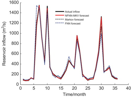
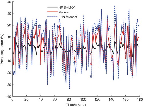
Figure 3. Percentage errors of three forecasting models from January 2009 to December 2011.

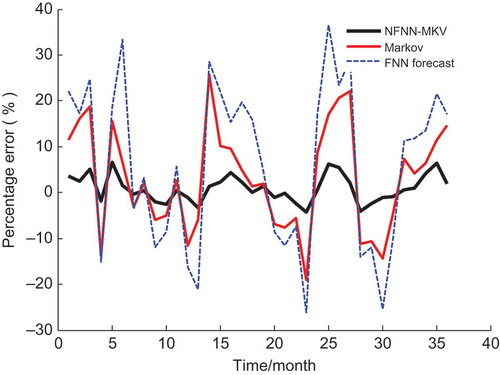
Figure 4. Actual monthly inflows and forecast monthly inflows of the NFNN-MKV model from January 1999 to November 2013.

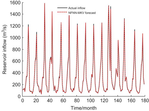
Figure 5. Percentage errors of three forecasting models from January 1999 to November 2013.

Table 10 shows that the predicted monthly inflows for the NFNN-MKV model are better than those for the Markov model and the FNN model. The predicted monthly inflow for the NFNN-MKV model is closer to the actual value in each month. The APE for the NFNN-MKV model is smaller than that for the Markov model and the FNN model in each month. The prediction precision of the NFNN-MKV model is higher than that of the other forecasting models in terms of PE.

Table 11 gives the reservoir’s prediction results for three forecasting models in 23 months, which are also the evaluated results of the NFNN-MKV, Markov and FNN model performances from January 2012 to November 2013.

Tables 10 and 11 show that the PE and APE of the NFNN-MKV model are lower than those of the other forecasting models in each month. The APE of the NFNN-MKV model does not exceed 7% in each period, the MAPE is less than 3.4%, and the MSE is 3.706. But the MAPE of the Markov model is higher than11%, the MSE is higher than 13.0, and the qualified rate is 82.6%. The MAPE of the FNN model is higher than 17%, the MSE is higher than 19.0, and the qualified rate is 60.9%. The MAPE and MSE of the NFNN-MKV model are lower than those of the other forecasting models. The PE of the NFNN-MKV model is relatively uniform, the floating range of its APE is 0–7.0%, and the qualified rate is 100%. This indicates that the NFNN-MKV model has much better prediction results than the Markov model and the FNN model in terms of MSE, MAPE, PE and APE. It shows that prediction accuracy of the NFNN-MKV model is higher than that of the Markov and FNN models. For further comparison of these better models, the maximum APE (Max-APE) and minimum APE (Min-APE) of the forecasting models, called the extreme error indices, were considered. The Max-APE (33.283) and Min-APE (4.998) of the FNN proved that this model had weaker prediction ability than the NFNN-MKV model (Table 10).

Figure 2 shows the contrast curve of actual monthly inflows and predicted monthly inflows for the NFNN-MKV model, the Markov model and the FNN model from January 2009 to December 2011.

Figure 3 shows the contrast curve of percentage errors for the NFNN-MKV, Markov and FNN forecasting models from January 2009 to December 2011.

Figure 4 shows the contrast curve of actual monthly inflows and predicted monthly inflows of the NFNN-MKV model from January 1999 to November 2013.

Figure 5 shows the contrast curve of percentage errors for the NFNN-MKV, Markov and FNN forecasting models from January 1999 to November 2013.

The prediction ability of the NFNN-MKV model is superior to that of the Markov and FNN models, as indicated by direct comparison of prediction results and observed data (Figs 2–5). Figures 2–5 and Tables 10 and 11 show that the predicted monthly inflows of the NFNN-MKV model are closer to the actual monthly inflows in all periods. The prediction precision of the NFNN-MKV model is higher than that of the Markov and FNN models. Figures 2 and 4 show that the percentage errors of the NFNN-MKV are smaller than those of the Markov and FNN models. The percentage error of the NFNN-MKV model is relatively uniform, and the floating range of its APE is 0–7.0%. This shows that the NFNN-MKV model is stable, and has higher prediction accuracy. Comparison of extreme error (Max-APE = 6.949, Min-APE = 0.679) indices indicates that the NFNN-MKV model is able to accurately forecast mid- to long-term runoff of rivers and reservoirs. Comparing the evaluation indices of the NFNN-MKV, Markov and FNN models, in terms of the smallest errors (MSE = 3.706, MAPE = 3.317, Max-APE = 6.949, Min-APE = 0.679), reveals that the NFNN-MKV model has the best performance to estimate general river and peak discharge. The NFNN-MKV model is suitable for mid- to long-term runoff prediction for rivers and reservoirs with respect to targets.

Table 12 shows forecast monthly inflow accuracy rates (FAR) for the NFNN-MKV model from January 2010 to November 2013.

Table 12. Forecast monthly inflow accuracy rate (FAR) of NFNN-MKV model for the Si Quan Reservoir.

Date (Y/M)	Accuracy rate (%)	Date (Y/M)	Accuracy rate (%)	Date (Y/M)	Accuracy rate (%)	Date (Y/M)	Accuracy rate (%)
2010/1	97.4	2010/2	98.7	2010/3	97.3	2010/4	94.4
2010/5	97.2	2010/6	98.1	2010/7	94.8	2010/8	97.3
2010/9	97.1	2010/10	96.5	2010/11	97.1	2010/12	97.2
2011/1	95.6	2011/2	96.1	2011/3	98.2	2011/4	96.3
2011/5	97.3	2011/6	97.8	2011/7	97.5	2011/8	96.9
2011/9	98.4	2011/10	98.1	2011/11	97.5	2011/12	96.1
2012/1	95.8	2012/2	94.7	2012/3	99.1	2012/4	96.6
2012/5	96.6	2012/6	99.2	2012/7	99.3	2012/8	94.2
2012/9	97.8	2012/10	96.5	2012/11	96.4	2012/12	97.2
2013/1	96.7	2013/2	95.2	2013/3	97.2	2013/4	96.5
2013/5	95.7	2013/6	96.3	2013/7	95.5	2013/8	95.7
2013/9	96.8	2013/10	98.8	2013/11	98.6

Table 12 shows that the accuracy rate for the NFNN-MKV model is about 96% from the continuous 47 months, the lowest accuracy rate is 94.2%, and the highest accuracy rate is 99.3%. The prediction accuracy has been significantly improved. This proves that the NFNN-MKV model has good prediction performance.

4 Application comparison of hybrid algorithm

4.1 Data and parameters

The datasets used for this comparison study include monthly rainfall and monthly river discharge time series for Weijiabao, referred to hereafter as the WJ series. The WJ series includes 696 months (58 years) of data from January 1956 to December 2013. The dataset was divided into three parts for network training, testing and prediction. We reserved the first 420 months (January 1956 to December 1990) of the data series for network training, used 120 months (January 1991 to December 2000) of the data series for network prediction testing, and used the rest (156 months: January 2001 to December 2013) of the data for prediction.

We compare the model fitting and prediction performance of the ideal point fuzzy neural network–Markov hybrid algorithm (NFNN-MKV) through selecting the wavelet–ANN (WNN) model (Wei et al. 2012, 2013) and the support vector regression (SVR) model (Behzad et al. 2009) with good performances. The performance of the method is validated via out-of-sample comparisons using real data from the runoff systems of Weijiabao. The performance of the NFNN-MKV method is tested by comparing the modelling results of the training, testing and prediction with the WNN model and the SVR model.

In this context, we used the previous 12-month data (average monthly rainfall and average monthly discharge) as inputs and the following 12-month data (monthly inflow) as the targets for neural network training (Table 9).

The structure of the neural network is as follows: there are 24 input layer nodes (average monthly rainfall, average monthly discharge); hidden layer nodes are determined by the test method; and the output layer has 12 nodes representing the targets for the following 12-month data (monthly inflow).

4.2 Simulation results

In the experiment, we adopt the monthly flow time series for Weijiabao to verify the effectiveness of the learning and forecasting for the NFNN-MKV method, the WNN model and the SVR model. The criteria used to compare the performance are the mean absolute percentage error (MAPE), the percentage error (PE), the absolute percentage error (APE) and the mean square error (MSE) in this paper, which indicate the accuracy of recall. In addition, for comparative study, numerical simulations comparing with the WNN and SVR methods are also conducted. First, according to the training, testing and prediction stages, we calculate the PE, MAPE, APE and MSE for three forecasting models. At the same time, to verify the effectiveness of the NFNN-MKV method, the performance of the proposed approach is studied.

Numerical results from the NFNN-MKV, WNN and SVR models are shown in Fig. 6 and 7 and Tables 13–15.

Table 13. Evaluation of the NFNN-MKV, WNN and SVR model performances for the whole training stage from January 1956 to December 1990.

Item	Model	MAPE (%)	Max-APE (%)	Min-APE (%)	MSE ((m^3/s)^2)
Training 1956–1990 (420 months)	NFNN-MKV	3.037	5.970	0.053	3.383
	WNN	9.627	26.475	0. 624	10.982
	SVR	17.579	36.652	1.946	18.929

Table 14. Evaluation results of the NFNN-MKV, WNN and SVR model performances in prediction testing stage from January 1991 to December 2000.

Item	Average actual monthly discharge (m^3/s)	Average prediction testing monthly discharge (m^3/s)	MAPE (%)	Max-APE (%)	Min-APE (%)	MSE ((m^3/s)^2)
NFNN-MKV	92.756	93.307	3.033	7.751	0.015	3.568
WNN	92.756	96.567	9.514	27.862	1.264	11.756
SVR	92.756	96.568	18.494	37.209	4.075	20.028

Table 15. Evaluation results of the NFNN-MKV, WNN and SVR model performances for the forecasting stage from January 2001 to December 2013.

Item	Average actual monthly discharge (m^3/s)	Average forecast monthly discharge (m^3/s)	MAPE (%)	Max-APE (%)	Min-APE (%)	MSE ((m^3/s)^2)
NFNN-MKV	140.397	140.59	2.768	5.904	0.0447	3.256
WNN	140.397	140.066	8.158	21.749	0.0064	9.952
SVR	140.397	141.704	16.954	35.797	2.8057	18.389

Figure 6. Comparison of simulated results and observed actual data of the NFNN-MKV, WNN and SVR models.

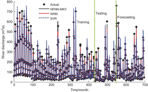
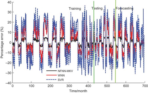
Figure 7. Comparison of simulated results and the percentage errors of the NFNN-MKV, WNN and SVR models.

The visualized comparison of the simulated and observed discharge series between the NFNN-MKV, WNN and SVR models is illustrated in Fig. 6. This figure clearly illustrates that, comparing the NFNN-MKV, WNN and SVR models, each model had very good performance for fitting historical data during training, but the simulated results of the NFNN-MKV model are closer to the actual monthly discharges in the training, testing and forecasting periods, so are better than those of the WNN and SVR models.

The general training, testing and forecasting evaluation results of the NFNN-MKV, WNN and SVR models using the observed discharge data and the percentage errors are showed in Fig. 6 and 7. Comparing the results shown in Fig. 6 and 7 indicates that the performance of the NFNN-MKV model is better than the WNN and SVR models. The percentage errors of the NFNN-MKV model are smaller in all periods, so better than those of the WNN and SVR models. The percentage errors for the NFNN-MKV model are relatively uniform, and the floating range of its APE is 0–6.0%, which indicates that the stability and robustness of the NFNN-MKV model are better than those of the WNN and SVR models.

The MAPE, Max-APE, Min-APE and MSE of the three models for performance comparison over the whole training stage from January 1956 to December 1990 are summarized in Table 13.

In general, the results show that the NFNN-MKV, WNN and SVR models meet the performance goal quickly. Comparison of the training results of the NFNN-MKV, WNN and SVR models suggests that they have very good simulated performances in terms of MAPE, Max-APE, Min-APE as well as MSE. However, the training results of the NFNN-MKV model with smaller errors (MAPE = 3.037%, Max-APE = 5.97%, Min-APE = 0.053% and MSE = 3.383) show that this model has the best performance for fitting historical data, better than that of the WNN and SVR models.

The general testing evaluation results for model prediction ability of the NFNN-MKV, WNN and SVR models using the observed discharge data from January 1991 to December 2000 are summarized in Table 14. In terms of MAPE, Max-APE, Min-APE and MSE, the NFNN-MKV, WNN and SVR models exhibit good correlation between observed data and simulated results. However, the NFNN-MKV model has much better prediction results than the WNN and SVR models in terms of MAPE, Max-APE, Min-APE, MSE as well as average prediction testing monthly discharge.

Table 15 shows a comparison between the NFNN-MKV approach and two other approaches (WNN and SVR models) regarding the MAPE, Max-APE, Min-APE and MSE criteria. The NFNN-MKV approach presents better forecasting accuracy: the MAPE, Max-APE, Min-APE and MSE over the forecasting months (156 months: from January 2001 to December 2013) for Weijiabao on the Weihe River have values of 2.768%, 5.904%, 0.0447% and 3.256(m³/s)², respectively. Improvement in the MAPE of the NFNN-MKV approach with respect to the WNN and SVR models is 66.1% and 83.6%, respectively. Improvement in the Max-APE of the NFNN-MKV approach with respect to the WNN and SVR models is 72.9% and 83.5%, respectively. Improvement in the MSE of the NFNN-MKV approach with respect to the WNN and SVR models is 67.3% and 82.3%, respectively. From the three tables and two figures, clearly the NFNN-MKV outperforms the WNN and SVR models in almost all situations. It can be seen that the NFNN-MKV approach is much better than the WNN and SVR models and can be considered high in terms of accuracy.

Figures 6 and 7 and Tables 13–15 show that the NFNN-MKV, WNN and SVR models have very good performance for fitting historical data during training, testing and prediction, but the NFNN-MKV model values are closer to the actual monthly discharges in all periods, better than those of the WNN and SVR models. In terms of MAPE, Max-APE, Min-APE and MSE, the stability and robustness of the NFNN-MKV model are better than those of the WNN and SVR models; the former has the higher prediction accuracy.

5 Conclusions

In this paper, a mid- to long-term runoff forecasting model has been developed using an ideal point fuzzy neural network–Markov (NFNN-MKV) hybrid algorithm to improve the forecasting precision. Prediction application results for the Si Quan Reservoir show that the NFNN-MKV hybrid algorithm has good performance in terms of faster convergence, better forecasting accuracy and significant improvement of neural network generalization in comparison with the traditional fuzzy neural network or Markov models. The absolute percentage error of the NFNN-MKV hybrid algorithm is less than 7.0%, MSE is less than 3.9, and qualification rate reaches 100%.

Another comparison case study illustrates the performance of the NFNN-MKV hybrid algorithm to improve forecasting accuracy. The NFNN-MKV, WNN and SVR models have been employed to estimate (training (420-month) and testing for 120-month-ahead prediction) and predict river discharge (156 months). Numerical comparison results confirm the efficiency of the NFNN-MKV method, which indicates that the NFNN-MKV model is able to significantly increase prediction accuracy. The NFNN-MKV approach presents better forecasting accuracy: the MAPE, Max-APE, Min-APE and MSE over the forecasting months (156 months: from January 2001 to December 2013) for Weijiabao on the Weihe River have values of 2.768%, 5.904%, 0.0447% and 3.256 (m³/s)², respectively. In terms of MAPE, Max-APE, Min-APE and MSE, the stability and robustness of the NFNN-MKV model are better than those of the WNN and SVR models; the former has the higher prediction accuracy. The NFNN-MKV model takes the advantages of the ideal point fuzzy neural network and the Markov prediction model, which can solve the problem of a stationary or volatile strong random process. The NFNN-MKV hybrid algorithm enhances the efficiency of mid- to long-term runoff forecasting for a reservoir system, and it is a scientific and effective forecasting model. The mid- to long-term runoff forecasting method based on the NFNN-MKV hybrid algorithm has promotional values.

Disclosure statement

No potential conflict of interest was reported by the authors.

Additional information

Funding

This work was financially supported by the China National Funds for Distinguished Young Scientists (61025014), National Natural Science Foundation (61304001), the China Ministry of Science Technology Innovation Funds (12C26213714122), the China Ministry of Industry and Information Technology Special Funds ([2011] 353), the Ning Xia Natural Science Funds (NZ12112), the Ning Xia Department of Education Reform Project Funds ([2012] 348), the China Postdoctoral Science Foundation (2012M512147), the China Postdoctoral Science Special Foundation (2013T60929) and Innovation team project of Chang Jiang Scholars and Innovative Research Team of Ministry of Education (IRT1067).

References

- Adamowski, J., et al., 2012. Comparison of multivariate adaptive regression splines with coupled wavelet transform artificial neural networks for runoff forecasting in Himalayan micro-watersheds with limited data. Journal of Hydroinformatics, 14, 731. doi:10.2166/hydro.2011.044
- Adamowski, J. and Sun, K., 2010. Development of a coupled wavelet transform and neural network method for flow forecasting of non-perennial rivers in semi-arid watersheds. Journal of Hydrology, 390 (1–2), 85–91. doi:10.1016/j.jhydrol.2010.06.033
- Anctil, F. and Tape, D.G., 2004. An exploration of artificial neural network rainfall-runoff forecasting combined with wavelet decomposition. Journal of Environmental Engineering and Science, 3 (S1), S121–S128. doi:10.1139/s03-071
- Andrews, R., et al., 2001. A review of techniques for extracting rules from trained artificial neural networks. Clinical Applications of Artificial Neural Networks, 256–297. doi:10.1017/CBO9780511543494.012
- Aqil, M., et al., 2007. A comparative study of artificial neural networks and neuro-fuzzy in continuous modeling of the daily and hourly behaviour of runoff. Journal of Hydrology, 337 (1–2), 22–34. doi:10.1016/j.jhydrol.2007.01.013
- Behzad, M., et al., 2009. Generalization performance of support vector machines and neural networks in runoff modeling. Expert Systems with Applications, 36 (4), 7624–7629. doi:10.1016/j.eswa.2008.09.053
- Bolch, G., et al., 2006. Queueing networks and Markov chains: modeling and performance evaluation with computer science applications. Hoboken, NJ: John Wiley & Sons.
- Chang, F., Chang, L.-C., and Huang, H.-L., 2002. Real-time recurrent learning neural network for stream flow forecasting. Hydrological Processes, 16 (13), 2577–2588. doi:10.1002/hyp.1015
- Deka, P. and Chandramouli, V., 2003. A fuzzy neural network model for deriving the river stage-discharge relationship. Hydrological Sciences Journal, 48 (2), 197–209. doi:10.1623/hysj.48.2.197.44697
- Dibike, Y.B. and Solomatine, D.P., 2001. River flow forecasting using artificial neural networks. Physics and Chemistry of the Earth, Part B: Hydrology, Oceans and Atmosphere, 26 (1), 1–7. doi:10.1016/S1464-1909(01)85005-X
- Elshorbagy, A., Simonovic, S.P., and Panu, U.S., 2000. Performance evaluation of artificial neural networks for runoff prediction. Journal of Hydrologic Engineering, 5 (4), 424–427. doi:10.1061/(ASCE)1084-0699(2000)5:4(424)
- Gardner, L.R., 2009. Assessing the effect of climate change on mean annual runoff. Journal of Hydrology, 379 (3–4), 351–359. doi:10.1016/j.jhydrol.2009.10.021
- Guo, X., et al., 2010. Study on prediction model of the chaotic runoff time series using fuzzy support vector machines and a case study. Shuili Fadian Xuebao (Journal of Hydroelectric Engineering), 29 (3), 51–55.
- Hlynka, M., 2007. Queueing networks and markov chains (modeling and performance evaluation with computer science applications). Technometrics, 49 (1), 104–105. doi:10.1198/tech.2007.s457
- Hong, W.-C. and Pai, P.-F., 2007. Potential assessment of the support vector regression technique in rainfall forecasting. Water Resources Management, 21 (2), 495–513. doi:10.1007/s11269-006-9026-2
- Hu, X.J., et al., 2012. Index of multiple factors and expected height of fully mechanized water flowing fractured zone. Journal of China Coal Society, 4, 016.
- Jackson, A., 2009. Markov Analysis with Non-constant Hazard Rates. Thesis (Master). California State University.
- Jain, A. and Kumar, A.M., 2007. Hybrid neural network models for hydrologic time series forecasting. Applied Software Computing, 7 (2), 585–592. doi:10.1016/j.asoc.2006.03.002
- Jothityangkoon, C., Sivapalan, M., and Viney, N.R., 2000. Tests of a space-time model of daily rainfall in southwestern Australia based on nonhomogeneous random cascades. Water Resources Research, 36 (1), 267–284. doi:10.1029/1999WR900253
- Kasabov, N.K. and Song, Q., 2002. DENFIS: dynamic evolving neural-fuzzy inference system and its application for time-series prediction. IEEE Transactions on Fuzzy Systems, 10 (2), 144–154. doi:10.1109/91.995117
- Kisi, O., 2010. Wavelet regression model for short-term stream flow forecasting. Journal of Hydrology, 389 (3–4), 344–353. doi:10.1016/j.jhydrol.2010.06.013
- Kisi, O., 2011. Wavelet regression model as an alternative to neural networks for river stage forecasting. Water Resources Management, 25 (2), 579–600. doi:10.1007/s11269-010-9715-8
- Kişi, Ö., 2009. Wavelet regression model as an alternative to neural networks for monthly stream flow forecasting. Hydrological Processes, 23 (25), 3583–3597. doi:10.1002/hyp.7461
- Kottegoda, N.T., Natale, L., and Raiteri, E., 2000. Statistical modeling of daily stream flows using rainfall input and curve number technique. Journal of Hydrology, 234 (3–4), 170–186. doi:10.1016/S0022-1694(00)00252-3
- Kwan, H.K. and Cai, Y., 1994. A fuzzy neural network and its application to pattern recognition. IEEE Transactions on Fuzzy Systems, 2 (3), 185–193. doi:10.1109/91.298447
- Li, Z., et al., 2010. Analysis of parameter uncertainty in semi-distributed hydrological models using bootstrap method: A case study of SWAT model applied to Yingluoxia watershed in northwest China. Journal of Hydrology, 385 (1–4), 76–83. doi:10.1016/j.jhydrol.2010.01.025
- Lin, J.-Y., Cheng, C.-T., and Chau, K.-W., 2006. Using support vector machines for long-term discharge prediction. Hydrological Sciences Journal, 51 (4), 599–612. doi:10.1623/hysj.51.4.599
- Maier, H.R., et al., 2010. Methods used for the development of neural networks for the prediction of water resource variables in river systems: current status and future directions. Environmental Modelling & Software, 25 (8), 891–909. doi:10.1016/j.envsoft.2010.02.003
- Marshall, L., Nott, D., and Sharma, A., 2004. A comparative study of Markov chain Monte Carlo methods for conceptual rainfall-runoff modeling. Water Resources Research, 40, 2. doi:10.1029/2003WR002378
- Moosavi, V., et al., 2013. A wavelet-ANFIS hybrid model for groundwater level forecasting for different prediction periods. Water Resources Management, 27 (5), 1301–1321. doi:10.1007/s11269-012-0239-2
- Nayak, P.C., et al., 2004. A neuro-fuzzy computing technique for modeling hydrological time series. Journal of Hydrology, 291 (1–2), 52–66. doi:10.1016/j.jhydrol.2003.12.010
- Nourani, V., et al., 2013. Using self-organizing maps and wavelet transforms for space-time pre-processing of satellite precipitation and runoff data in neural network based rainfall-runoff modeling. Journal of Hydrology, 476, 228–243. doi:10.1016/j.jhydrol.2012.10.054
- Pachet, F., Roy, P., and Barbieri, G., 2011. Finite-length Markov processes with constraints. In: Proceedings of the 22nd International Joint Conference on Artificial Intelligence, IJCAI. Menlo Park, CA: AAAI Press, 635–642.
- Partal, T. and Kişi, Ö., 2007. Wavelet and neuro-fuzzy conjunction model for precipitation forecasting. Journal of Hydrology, 342 (1–2), 199–212. doi:10.1016/j.jhydrol.2007.05.026
- Rong, H.-J., et al., 2006. Sequential adaptive fuzzy inference system (SAFIS) for nonlinear system identification and prediction. Fuzzy Sets and Systems, 157 (9), 1260–1275. doi:10.1016/j.fss.2005.12.011
- Shamseldin, A.Y., O’Connor, K.M., and Liang, G.C., 1997. Methods for combining the outputs of different rainfall-runoff models. Journal of Hydrology, 197 (1–4), 203–229. doi:10.1016/S0022-1694(96)03259-3
- Shi, B., 2009. Short-term load forecast based on modified particle swarm optimizer and back propagation neural network model. Journal of Computer Applications, 29 (4), 1036–1039. doi:10.3724/SP.J.1087.2009.01036
- Shi, B., 2010a. Short-term load forecasting based on modified particle swarm optimizer and fuzzy neural network model. System Engineering-Theory & Practice, 30 (1), 157–166.
- Shi, B., 2010b. Long-term runoff forecast method based on dynamic adjustment particle swarm optimizer algorithm and Holt-Winters linear seasonal model. Transactions of the CSAE, 26 (7), 8–13.
- Shiri, J. and Kisi, O., 2010. Short-term and long-term stream flow forecasting using a wavelet and neuro-fuzzy conjunction model. Journal of Hydrology, 394 (3–4), 486–493. doi:10.1016/j.jhydrol.2010.10.008
- Wang, C.-H. and Hung, K.-N., 2013. Intelligent adaptive law for missile guidance using fuzzy neural networks. International Journal of Fuzzy Systems, 15 (2), 182–191.
- Wang, Z., Liang, H., and Liu, G., 2005. Mid and long term hydrology forecast model and its application. Journal of Hydroelectric Engineering, 2, 008.
- Wei, S., Song, J., and Khan, N.I., 2012. Simulating and predicting river discharge time series using a wavelet-neural network hybrid modelling approach. Hydrological Processes, 26 (2), 281–296. doi:10.1002/hyp.8227
- Wei, S., et al., 2013. A wavelet-neural network hybrid modelling approach for estimating and predicting river monthly flows. Hydrological Sciences Journal, 58 (2), 374–389. doi:10.1080/02626667.2012.754102
- Wu, C.L., Chau, K.W., and Li, Y.S., 2008. River stage prediction based on a distributed support vector regression. Journal of Hydrology, 358 (1–2), 96–111. doi:10.1016/j.jhydrol.2008.05.028
- Xiong, L., Shamseldin, A.Y., and O’connor, K.M., 2001. A non-linear combination of the forecasts of rainfall-runoff models by the first-order Takagi–Sugeno fuzzy system. Journal of Hydrology, 245 (1–4), 196–217. doi:10.1016/S0022-1694(01)00349-3
- Yang, J.-S., Yu, S.-P., and Liu, G.-M., 2013. Multi-step-ahead predictor design for effective long-term forecast of hydrological signals using a novel wavelet-NN hybrid model. Hydrology & Earth System Sciences Discussions, 10, 9239–9269. doi:10.5194/hessd-10-9239-2013