Seasonal river flow forecasts for the United Kingdom using persistence and historical analogues

Abstract

Seasonal river flow forecasting methods are currently being developed for country-wide application in the United Kingdom, using several different techniques. In this paper, methods based on persistence and historical flow analogues are presented. New 1- and 3-month forecasts are made each month using monthly river flows at 93 stations with records at least 30 years long. The method that performs best is selected for each separate month, catchment and forecast duration. The forecasts based on persistence of the previous month’s flow generally outperform the analogues approach, particularly for slowly responding catchments (mainly in the southeast) with large underground water storage in aquifers. Historical analogues make a useful contribution to the forecasts in the northwest of the country. Correlations between hindcasts and observations that exceed 0.23 and are significant at the 5% level for a one-sided test are found for 81% (70%) of the station–month combinations for the 1-month (3-month) forecast.

Editor Z. W. Kundzewicz Associate editor Not assigned

Keywords:

• Seasonal forecasting
• river flow
• persistence
• historical analogue
• United Kingdom

1 Introduction

Predictions of water availability on a seasonal time scale are useful for managers and planners involved in a range of activities, such as agriculture, water supply and reservoir management. In the United Kingdom (UK), the development of seasonal river flow forecasting methods has previously been limited to either a few catchments, and/or covered mainly the summer season (e.g. Wilby 2001, Wedgbrow et al. 2002, 2005, Wilby et al. 2004, Svensson and Prudhomme 2005). These methods are all based on empirical relationships between hydrological indicators and climate indices in the preceding months, and are therefore not easily transferrable to other locations and seasons.

The recent long-lasting drought (2010–2012) and its spectacular termination leading to major flooding (e.g. Marsh et al. 2013) have prompted a renewed interest in seasonal hydrological forecasting in the UK. A range of methods for application year-round and nationwide is currently being developed jointly by the Centre for Ecology & Hydrology (CEH), the British Geological Survey, the UK Met Office and the UK environment agencies (Hydrological Outlook UK, http://www.hydoutuk.net/). These methods include river flow and groundwater modelling approaches using either seasonal rainfall forecasts or historical rainfall series as input. Akin to the previously developed empirical methods, regression-based models for river flow forecasting using large-scale forcings, such as sea surface temperatures and airflow indices, as predictors are also under development. However, this is a longer-term effort because new teleconnection patterns need to be identified for the different regions of the UK, and for all seasons.

As alternatives that are more straightforward to implement in the short-term, the present paper outlines approaches to flow forecasting based on flow persistence and historical flow analogues. The underlying assumption for the latter is that sequences of river flow in the historical record that are similar to the recent past will provide valuable information on what flows will occur in the near future. River flow can be seen as an aggregation of the rain falling onto the catchment and the evaporative losses from it, plus the change in storage. Over a succession of months, the rainfall and potential evaporation will depend on the state and evolution of large-scale atmospheric circulation patterns. The river flow response will depend also on the state and characteristics of the catchment (e.g. Sivapalan et al. 2005), and if no rain falls the rate of flow recession may be reasonably well-known. The underlying assumption for using analogues as a forecast method is that there are particular “trajectories” that the hydro-climatic system may follow, which may repeat themselves.

van den Dool (2007) provides a comprehensive discussion of the use of historical analogues for climate prediction. He concludes that although using a single “natural” analogue may have limited applicability, “constructed” analogues have been shown to be useful for forecasting. Here, a constructed analogue means an analogue derived based on the combination of a range of historical sequences rather than on a single sequence. In hydrology, Yao and Georgakakos (2001) selected several sequences from a historical record of inflows to a reservoir on the American River, California, and used the flows following the analogues as possible future realisations on which to base probabilistic multi-lead forecasts. Koutsoyiannis et al. (2008) formed the mean of the flow sequences following the selected historical analogues, and used this as a prediction of Nile River flows 1 month ahead. For the United States, van den Dool et al. (2003) made linear combinations of spatial fields of soil moisture at the same time of year in years past, to reproduce the initial condition at the end of the current month to within a small tolerance. The coefficients assigned to the years past were then made to persist, and the subsequent development in the historical years was linearly combined to form a forecast.

In the present study, two types of analogue forecast are used to predict mean river flows 1 and 3 months ahead. The forecasts are made each month of the year, at 93 individual river flow stations across the UK. First, for each (transformed) monthly flow series, the most similar analogues in the historical record compared with the flows observed in the most recent 6 or 9 months are found based on the root mean square error (RMSE). There is one potential analogue per year, as the season of each analogue is kept the same as the season of the recent past. A weighted mean forecast is then made by using the RMSEs to construct weights, which are applied to the flow sequences following the historical analogues. Second, a shifted weighted mean forecast is derived by increasing or decreasing the weighted mean forecast, so that the weighted mean flows in the last month of the historical analogues equals the flow in the last month of the recent past.

The slowly changing river flows in catchments with large groundwater stores means that simple persistence forecasts based on the last month’s observed river flow anomaly can be very successful. The use of anomalies allows the forecast to follow the seasonal cycle, rather than persisting a fixed flow value. Persistence forecasts are made together with the two historical analogues approaches, and the forecast method that performs best for each catchment and month is used.

2 Data and catchment selection

Daily mean river flow data from the National River Flow Archive were used. The selection of river flow stations was restricted by the requirement that they should be included in the National Hydrological Monitoring Programme (NHMP, http://www.ceh.ac.uk/data/nrfa/nhmp/nhmp.html), which means that CEH receives monthly updates for them (e.g. Dixon et al. 2013). This is necessary for obtaining the most recent months’ data up to the point of the start of the forecast, which is the time period used for comparison with the historical data and finding the analogues. Data are currently delivered by the 5th working day of the month (this is expected to soon become even earlier), and a brief quality check is carried out and any queries sent back to the provider. The stations in the NHMP programme have a generally good data quality. In total 93 stations in the UK were selected, all of which have at least 30 years of observations to 30 June 2013. The two earliest records commence in 1883. The bulk of the records start in the early 1960s, which is reflected in the median record length of 50.7 years and the mean of 51.8 years. The mean record length is reduced to 51.5 years when missing data are removed.

The flows in the selected catchments are not unduly influenced by reservoirs and lakes, having a value of Flood Attenuation of Reservoirs and Lakes (FARL) ≥ 0.9 (see Marsh and Hannaford (2008)). However, four stations were included in the study despite them not fulfilling this criterion: the Tay at Ballathie because it is the largest river in the country in terms of flow magnitude, and three stations in northwest Scotland (The Carron at New Kelso, the Ewe at Poolewe and the Naver at Apigill) to improve the spatial coverage. Considerable proportions of these latter three catchments drain through lakes, but the flow regimes are otherwise nearly natural (i.e. largely unaffected by abstractions, hydro-power schemes, etc.). Two stations fulfilling the above criterion were omitted: the Dee at Manley Hall because it has a maintained low flow, and the Usk at Trostrey Weir because it gauges low flows only. Naturalised flows are available and used for two of the stations: the Thames at Kingston and the Lee at Feildes Weir. The naturalised flow is the gauged river flow adjusted to take account of net abstractions and discharges upstream of the gauging station. Although these two catchments are the most affected, many of the other catchments are also subject to varying degrees of human influence. However, 31 of the catchments are part of the so called benchmark network (Bradford and Marsh 2003) and are relatively undisturbed.

3 Methods

Calculation of mean monthly flow anomalies

Monthly mean river flows were calculated for each station. The monthly means were calculated from daily mean flows, and data was set to missing for a month if there were fewer than 25 valid daily observations available. A log-transform was then carried out on the monthly mean flows. This makes the distribution of the flows more similar to a normal distribution, and when assessing the similarity of the analogues to the recent past, the very highest river flows become less outstanding.

Because river flow has a clear seasonal cycle both in the monthly mean and in the standard deviation, standardised river flow anomalies were used for the analysis and were calculated as follows. For each of the 12 calendar months, mon, the climatological mean flow, m_i, mon, and standard deviation, s_i, mon, were calculated for each station, i, from the log-transformed monthly mean flows, q_i, t. A series of standardised monthly anomalies, a_i, t, were then calculated as

(1)

Here, t denotes the serial number of the month, starting from January 1883, and mon refers to the calendar month that t pertains to.

Forecast methods

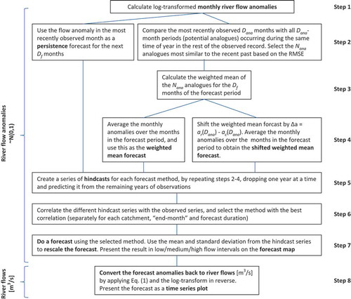
Forecasts can be made once all the data observations for the latest month, the “end-month”, have been received. Every month, three types of seasonal river flow forecasts are made: persistence of the previous month’s flow, and two types of historical analogue forecasts. Forecasts are made for the mean flow in the coming 1 and 3 months. For each catchment, “end-month” and forecast duration, the method that has performed best in the past is chosen. The methods are described in detail below, and a summary flowchart is provided in Fig. 1.

Figure 1. Flowchart summary of the forecasting methodology.

Persistence forecast

The persistence forecast uses the standardised anomaly from the most recent month with observations, and uses this anomaly as the forecast for the next 1 or 3 months. Hence, the seasonal cycle in the flows is preserved in the forecast.

Weighted mean analogue forecast

For the weighted mean analogue forecast, the monthly anomalies of the most recently past months are compared with all possible historical sequences of anomalies covering the same months of the year. That is, if the recent past covers, say, the months February to July, then potential analogues are sought only in the February to July sequences of the historical record. This means that there is one potential analogue available per year. From this annual series of potential analogues, the N_ana historical analogues most similar to the recent past are selected, based on the root mean square error (RMSE). The inverse of these RMSEs are then used to weight the flow anomalies in the months following the analogues, to form a weighted mean analogue forecast.

The RMSE is calculated for each potential analogue in the observed record, as

(2)

where a_p(k) is the flow anomaly for each month k in the potential analogue of duration D_ana, and a_r(k) is the corresponding flow anomaly in the recent past. When there is missing data in an analogue, or in the period following it that would be required for a forecast, that analogue is not included in the analysis.

The RMSEs for the selected N_ana analogues are used to calculate the weight, w, for each analogue, as

(3)

where b = 1, …, N_ana is the rank of the ordered RMSEs (the potential analogue a_p(b) with the smallest RMSE has rank b = 1). The weighted mean forecast anomalies, a_f(m), for each month m = 1, …, D_f in the forecast duration, D_f, form the last part of the constructed analogue, a_c, and are calculated as

(4)

where a_p,b is the vector of flow anomalies for the potential analogue with rank b.

When the forecast period, D_f, is longer than a month, the forecast anomalies are averaged over all the months in the forecast duration.

Because of the averaging over the number of analogues, and over the months in the 3-month forecast, the variance of the forecast flow anomaly will no longer be 1, it will be smaller. This means that a forecast will tend to be neither particularly high, nor particularly low, but rather middling (and therefore seemingly uninformative). This does not matter when assessing forecast performance using contingency tables or the correlation between hindcasts and observations, since in these cases the co-variation of the two series is the only consideration. However, it does matter for a forecast in absolute terms, when converting the forecast anomaly back to river flows (m³/s). If the anomalies have mean = 0 and standard deviation = 1, then the river flows can be obtained by reversing the standardisation of equation (1). Therefore, the variance of the forecast anomaly is re-inflated by re-standardising the anomalies to obtain mean = 0 and standard deviation = 1. This is done by subtracting the mean and dividing by the standard deviation of the record of hindcasts for the appropriate station and time of year. See the section on Jack-knife validation for further details on the hindcasts. The subtraction of the mean counteracts any bias that may result from the forecast method.

Shifted weighted mean analogue forecast

When, say, the river flow in the most recent month has been unusually or even unprecedentedly high, the selected analogues may fail to reflect the extremeness of the prevailing flow situation. In slowly responding catchments flows will take time to recede and the weighted mean analogue forecast is likely to be too low. In an attempt to take this discrepancy into account, a shifted weighted mean analogue forecast is carried out. That is, the weighted mean analogue forecast, before its re-standardisation, is shifted up or down. The magnitude and direction of the shift, Δa, depends on the flow anomaly in the last month of the constructed analogue, a_c(D_ana), which is moved so that it equals the observed flow anomaly in the most recent month, a_r(D_ana):

(5)

Although this shift means that the variance does not shrink as much as for the non-shifted forecast, it still needs re-standardising using the hindcasts to obtain a mean = 0 and standard deviation = 1. This is necessary for a correct conversion from anomalies back to flows (in m³/s).

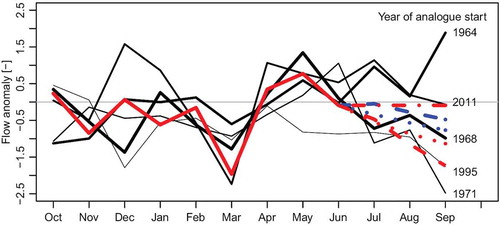
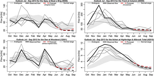
Figure 2 shows an example of flow anomalies for all three types of forecasts, for July to September 2013 at the Spey at Boat o Brig in northeast Scotland. The blue dashed line shows the weighted mean forecast based on the five analogues. The forecast anomaly is different for each month, as this plot shows intermediate results before the forecast is averaged across the months in the forecast period. The red dashed line shows the same forecast after the re-standardisation based on the hindcasts. The blue dotted line shows the shifted weighted mean forecast, and is shifted downwards from the blue dashed line, reflecting the difference between the observed flow and the weighted mean of the analogues in June. The red dotted line shows the shifted weighted mean forecast after it has been re-standardised based on the hindcasts. The dash-dotted red line shows the persistence forecast.

Figure 2. River flow forecasts (anomalies) for July to September 2013 for the Spey at Boat o Brig (hydrometric station number 8006), before averaging across the 3 months in the forecast period. The final forecasts are shown in red: weighted mean analogue (dashed line), shifted weighted mean analogue (dotted line) and persistence (dash-dotted line). Un-standardised forecasts for the analogues approaches are shown in blue. The five analogues (solid black lines) are shown with different line thickness depending on similarity to the recently observed flow (solid red line).

Jack-knife validation

For each calendar month, the forecast method that has shown the best performance for that “end-month” in the past is selected for making the monthly forecast. Performance is based on “jack-knife” hindcasts for the period of observations available at each station (30–130 years). This involves dropping 1 year at a time from the record, and forecasting the flow anomalies in this missing year using the remaining years in the record. In this way, a hindcast will be made for each year which can be compared with the flow anomaly that was actually observed in that year. For each method, the correlation between its hindcast record and the observed record is calculated for each calendar month, and is used as a measure of its performance. Contingency tables of the same anomaly series are also used for assessing the methods.

Re-standardisation of the forecasts using the hindcast series

The mean and standard deviation from the hindcast series are used to rescale the analogue forecast anomaly to have mean = 0 and standard deviation = 1 before it is converted back to flow (in m³/s). This brings about the question of whether or not to also re-standardise the persistence forecast. This should be done for consistency, to ensure that the forecast anomaly comes from a distribution with mean = 0 and standard deviation = 1, before converting it back to flows. Appendix 1 shows a worked example that illustrates the effects of the re-standardisation.

Individual stations versus regional analysis

Initially, the analysis was carried out for a range of clusters (up to five) of stations, rather than for individual stations. This was done because of a wish to obtain longer series by averaging the flows regionally, and to reduce noise in the forecasts. The clustering was based on the monthly flow anomalies. K-means and complete linkage methods both first divide the country into a hilly, windward region comprising catchments in the north and west, and a more sheltered lowland region in the south and east. When three clusters were used, the very slowly responding catchments, predominantly on the Chalk outcrop, were separated out from the southeast region. However, regardless of the number of clusters used, persistence was the predominant forecast method for most regions and months of the year. It therefore seemed sensible to make use of the local flow observations for the persistence forecasts by using individual stations rather than regional flows based on clusters of stations. (Similar to the results for using individual stations, forecasts for the northern and western regions were often not successful).

4 Results

Optimum number of analogues and analogue duration

The analogue forecasts can be made using different numbers of analogues of different durations. The performance of the various options (2, 3, 5, 7 and 9 analogues, and durations of 3, 6, 9 and 12 months) was assessed based on the correlations between the hindcast anomalies and the observed anomalies for all the stations and “end-months”.

The number of station-month combinations with (Pearson) correlations ≥0.23, that was significant at the 5% level for a one-sided test, was counted. The threshold 0.23 is the correlation for which a 51-year long series (a typical record length) is significant at the 5% level. Because the significance level has to be met, shorter records need to have a higher correlation in order to be counted. A one-sided test is applied because we are only interested in positive correlations. For these, the one-sided test with a 5% significance level rejects the null hypothesis of the correlation being smaller than 0 for the same station-months as a two-sided test would reject the null hypothesis of the correlation being equal to 0 at a 10% significance level.

To assess the performance of the different numbers of analogues and analogue durations, the number of significant forecasts was counted for each combination of number and duration. The counts vary from 896 to 911 for the 1-month forecasts and from 762 to 780 for the 3-month forecasts, when applying the counts to the forecast system as a whole (i.e. choosing the best method for each of the 12 “end-months” and 93 stations). This allows the analogues to be optimised for the catchments where they are actually used, rather than optimising them also for catchments where the persistence method performs better. Overall, the counts show that the analogue durations that result in the largest number of usable forecasts are the 6-month analogue for the 1-month forecast, and the 9-month analogue for the 3-month forecast. However, the number of analogues to use is less clear, and a pragmatic choice of using five analogues for both forecast durations was selected. Five analogues comprise 10% of all possible analogues for a typical 51-year long series.

Numbers and types of usable forecasts

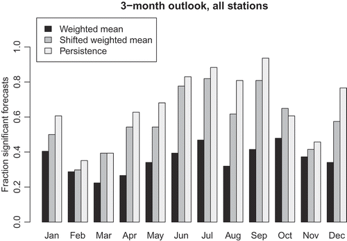
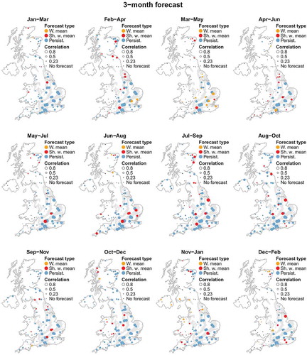
As discussed above, a forecast is considered to be usable if the correlation between the series of hindcast anomalies and observed anomalies exceeds 0.23 and is significant at the 5% level. When considering persistence forecasts only, usable forecasts can be made for 78% and 66% of station-month combinations for the 1- and 3-month forecast durations, respectively. The corresponding figures when using the best of the two historical analogue approaches are 70% and 59%. The ratios of usable forecasts for each method separately, for each forecast duration and time of year are shown in Figs 3 and 4. It can be seen that all methods generally perform better in the summer than in the winter.

Figure 3. Ratio of usable forecasts for each forecast method and time of year, for the 1-month forecast duration. The time of year denotes the last month of observations, i.e. the bars for January show the ratios for the February forecasts.

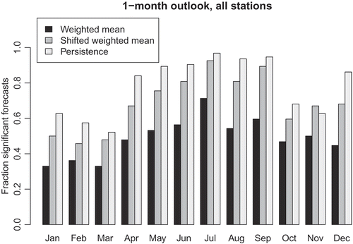
Figure 4. Ratio of usable forecasts for each forecast method and time of year, for the 3-month forecast duration. The time of year denotes the last month of observations, i.e. the bars for January show the ratios for the February–April forecasts.

When selecting the best option from all three approaches, usable forecasts can be made for 81% and 70% of station–month combinations for the 1-month and 3-month forecasts, respectively. The bulk of these are persistence forecasts. The historical analogues make up roughly the same number for the 1- and 3-month durations (about 13%), whereas the success rate of the persistence forecasts drops for the longer duration. Out of the number of usable forecasts only, historical analogue forecasts therefore make up 16% and 19% for the 1-month and 3-month duration, respectively.

Forecasts that are too uncertain to be made use of are mainly for locations in northwest Britain and in Northern Ireland (Figs 5 and 6). The 3-month forecasts are poor for many months of the year in these areas. The best forecasts are for the slowly responding permeable catchments draining the aquifer outcrop areas in the south and east of Britain, largely with correlations exceeding 0.5. The very best correlations are for the Chalk outcrops, where correlations reach 0.9 and above for several catchments. The highest correlations are 0.98 and 0.96 for the 1-and 3-month forecasts, respectively. The bulk of the forecasts for the groundwater-fed southeastern catchments are persistence forecasts. The historical analogues make useful contributions to the few usable forecasts in the north and west, particularly in autumn and winter.

Figure 5. One-month mean river flow forecasts for all months of the year. Different forecast methods are used for each individual location and are shown using different marker colours: orange denotes the weighted mean analogue forecast, red denotes the shifted weighted mean analogue forecast, and blue denotes the persistence forecast. The correlation between hindcasts and observations are shown by the size of the marker. Principal aquifer outcrops are shown using grey shading.

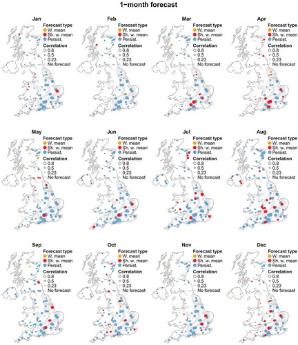
Figure 6. As for Fig. 5, but for the 3-month forecast.

Negative persistence

There seems to exist a weak to moderately strong negative relationship (correlation ≤ −0.23) between flow in February and flow in the following 3 months, for a dozen catchments in the mountainous north and west (marked with green dots in Fig. 7). Two such negative correlations also occur between flow in March and in the following 3 months, and for two catchments in west Scotland for flow in June and flows in the next 3 months. The spring-time correlations may be related to snow-melt, and the summer-time ones to problems with low flow measurements. In winter, precipitation may fall as snow which remains on the ground for some considerable time rather than produce an immediate runoff response. Come spring the accumulated snow will melt, resulting in a negative correlation between the suppressed winter flows and the subsequent high spring flows. Negative correlations do not occur for the 1-month forecast duration, except for one of the west Scotland catchments, between flow in June and July. These negative relationships have not been used for forecasting, because the reasons behind them have not been fully explored. However, the bottom left panel of Fig. 8 shows an example of spring-time high river flows in the Dee at Woodend (the northernmost green dot on the left panel of Fig. 7), which drains the Cairngorm Mountains in northeast Scotland. This is a catchment known to be strongly influenced by patterns of snow accumulation and melt (e.g. Baggaley et al. 2009). The high flow in Fig. 8 was associated with observed April precipitation exceeding the climatological average at Braemar in the upper reaches of the Dee catchment (64.0 and 54.3 mm/month, respectively). However, it followed a colder than average winter and early spring with average daily maximum temperatures only a few degrees above zero (http://www.metoffice.gov.uk/public/weather/climate-historic/#?tab=climateHistoric), which indicate that snow is also likely to have played a part.

Figure 7. Similar to Fig. 6, but also showing negative persistence forecasts (green).

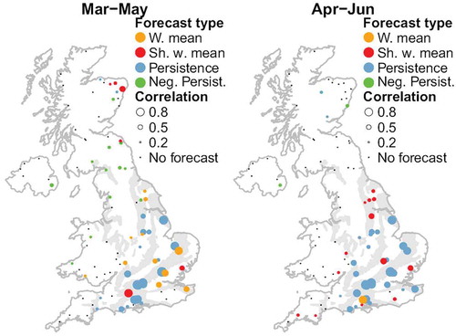
Figure 8. The July to September 2013 river flow forecast for the Spey at Boat o Brig (top left), the Dee at Woodend (bottom left), the Trent at Colwick (top right) and the Itchen at Highbridge & Allbrook Total (bottom right) shown as time series. The numbers in parentheses in the figure titles are the hydrometric station numbers. Which forecast method has been used in each case is stated on each diagram, and the forecasts are shown as red dashed lines. The actual flows that occurred are shown as dashed black lines. The recent past (thick solid black line) and the five closest historical analogues (thin solid black lines) are also shown. The area shaded grey shows the normal range of monthly river flows, i.e. the middle 44% of the empirical distribution of observed flows for the recent past, and the middle 44% of the empirical distribution of the hindcast flows for the forecast period.

Illustrative examples

Figure 8 shows river flow forecasts as monthly time series plots for a selection of catchments. The panels on the left show forecasts based on analogue methods, and in both cases the forecasts are near the lower envelope of the analogues. For the Spey (Fig. 8, top left) in northeast Scotland (yellow dot in Fig. 6 July–September forecast), the downward adjustment is due to the re-standardisation using the hindcasts, as the original weighted forecast lies just above the middle analogue (see Fig. 2). The bottom left panel of Fig. 8 shows the shifted weighted mean forecasts for the Dee, also located in northeast Scotland (the northernmost green dot in the left panel of Fig. 7). Here, the downward adjustment is due mainly to the shift aligning the forecast to the most recent flow observation, with the re-standardisation making a smaller contribution. The panels on the right in Fig. 8 show persistence forecasts, although the individual historical analogues are shown as well. There is not necessarily much difference in performance between the persistence forecast and the historical analogues for these examples of large (the Trent in central England, top right panel) or permeable (the Itchen in southern England, bottom right panel) catchments, but as discussed above persistence tends to do better overall.

Precision of the forecasts

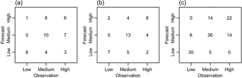
The historical analogues approach has the advantage that a range of outcomes is provided, which gives an indication of the uncertainty in the estimates. As can be inferred from the diagrams in Fig. 8 the uncertainty can be large, particularly in more quickly responding catchments. An alternative way of presenting the forecast precision, which can be applied to any type of forecast, is as a contingency table (Fig. 9). These tables cross-reference the hindcast flow anomalies with the actual observed flow anomalies. Here, flows are lumped into one of three intervals: high, medium and low. The intervals comprise the highest 28% of flows, the middle 44% of flows, and the lowest 28% of flows (in the empirical distributions). For the hindcasts, the 28th and 72nd percentiles come from the jack-knife validation, whereas for the observed flows the interval limits are based on the observed flow series. It can be noted that the use of the shifted forecast and the persistence forecast means that forecasts can be made that exceed the historical envelope of observations.

Figure 9. Examples of contingency tables. The corresponding correlations between hindcasts and observations are (a) 0.24, (b) 0.50 and (c) 0.83.

The middle interval of the contingency table spans the same percentiles as the middle interval (the “normal range”) in the monthly UK Hydrological Summary (http://nrfa.ceh.ac.uk/monthly-hydrological-summary-uk), whereas the various intervals for increasingly higher/lower flows in the Summary have been collapsed into single intervals for high and low flows, respectively. The Summary shows what river flows occurred across the UK in the previous month, and provides a source for continuous verification of the forecast provided in the Hydrological Outlook.

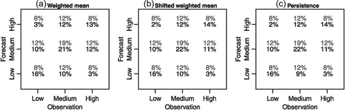
If all hindcasts were perfect, then all counts would be in the boxes along the diagonals, i.e. the number of hindcast low (medium/high) flows would be the same as the number of observed low (medium/high) flows. For correlations just above 0.23, there is still a large proportion of the hindcast flows which does not occur in the correct interval (Fig. 9). Instead, they occur in the neighbouring interval, and to a lesser extent in the opposite interval (for example, a high flow is predicted when, in fact, a low flow is observed). Although a correlation of 0.23 explains only about 5% of the variability, the contingency table shows that there is already some skill in avoiding the prediction of the opposite extreme. For correlations exceeding 0.7, more than 50% of the variability is explained and the risk of predicting the opposite extreme becomes smaller. The examples in Fig. 9 suggest that the risk of unpredicted extremes occurring is greatest when normal flow has been predicted. This is confirmed by Fig. 10, which shows the contingency tables for the 3-month forecast duration for the network as a whole for each method separately. Here, all stations and times of year for which there are usable forecasts have been lumped together. It can be seen that there is not much difference in precision between the methods once the non-usable forecasts have been removed. Overall, the bins for predicting the correct extreme have about twice as many occurrences as would be expected by chance, whereas the bins for predicting the wrong extreme only have about a third as many occurrences as expected by chance. The corresponding tables for the 1-month forecast are only very marginally better (not shown).

Figure 10. Contingency tables for the 3-month forecast duration for the network as a whole for (a) the weighted mean, (b) the shifted weighted mean and (c) the persistence methods. The tables are shown as percentages, with the expected percentages from a random distribution shown in grey.

Influence of record length on skill

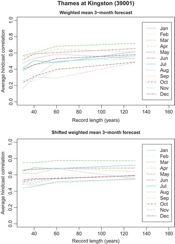
Longer records should make it more likely that better analogues are found. The longest flow record, the Thames at Kingston, starts in 1883 and was used to assess how performance improves with the number of years. Figure 11 shows the correlations between the hindcasts and observations vs record length for the two historical analogue methods, for the 3-month forecast duration. Non-overlapping subsets of 30-, 40- and 60-year periods were chosen, in addition to the full 130-year long record, and correlations were averaged for each record length. Figure 11 reveals that most of the increases in correlation have occurred by the time the record lengths reach 60 years. Because the median record length in the present study is about 51 years, the analogue methods may not yet have reached their full potential. The improvement with time is clearer for the weighted mean method, whereas the persistence element of the shifted weighted mean method means that this approach is comparatively good already for short records. The correlations for the 1-month forecast duration (not shown) are slightly higher than for the 3-month duration, but display similar features.

Figure 11. Correlation between hindcasts and observations vs record length for the Thames at Kingston, for the 3-month forecast duration for the weighted mean analogue method (top) and the shifted weighted mean analogue method (bottom).

The operational forecast map

At the beginning of each month, forecasts for the average flow in the coming 1 and 3 months are made. The main way of presenting the forecasts for the operational Hydrological Outlook is on a map showing whether flows are in the low, medium (“normal”) or high interval (Fig. 12). The forecast at each river gauging station is shown as a dot of a particular colour and size. The colour represents the hindcast flow (anomaly) magnitude interval, using the same percentiles for the interval limits as was used for the contingency tables. The size represents the confidence in the forecast, and is based on the correlations between the hindcast anomalies and the observed anomalies. Results are only presented on the forecast map provided that the correlation between the hindcast and the observed flow anomalies exceed 0.23, and that the correlation is significant at the 5% level (one-sided test).

Figure 12. Monthly mean river flow forecast for the United Kingdom for July 2013, using data up to the end of June 2013.

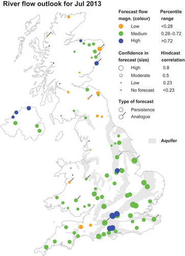
The actual river flows that occurred in July 2013 are shown on the UK Hydrological Summary web page: http://nrfa.ceh.ac.uk/monthly-hydrological-summary-uk. The general patterns of high, medium and low flows across the UK in the July Summary agree with the forecast, although several individual stations have river flows in the neighbouring intervals. Again, note that the interval for medium (“normal”) flows is the same for the Outlook and the Summary, but that the increasingly higher/lower intervals in the Summary have been collapsed into single intervals for high and low flows, respectively, for the Outlook.

5 Discussion

Year-round seasonal flow forecasting methods have only recently become available for the UK (or parts thereof). The present study covers all of the UK, is spatially resolved to individual catchments, and is validated using the correlation between the hindcasts and the observations and using contingency tables. In addition, two more methods for seasonal flow forecasting have been developed within the same cooperation project, as mentioned in the Introduction. Both these methods use hydrological rainfall–runoff models with ensemble inputs, and provide results in a probabilistic framework.

One- and three-month river flow forecasts are provided by running a grid-based rainfall–runoff model (Bell et al. 2013) with the UK Met Office 1- and 3-month ensemble rainfall forecasts as input. Spatially, these rainfall forecasts are currently only available as a single value for the entire country, and the river flow forecasts are presented as regional averages for 17 geographical regions of Great Britain (i.e. not including Northern Ireland).

Forecasts of average river flows 3–12 months ahead (part of the Forward look—river flows in the Environment Agency’s Water Situation Report, http://www.environment-agency.gov.uk/research/library/publications/33995.aspx) are provided by running rainfall–runoff models for about 30 key individual catchments in England only, using ensembles of historical sequences (climatology) of rainfall as input.

At present, the performance of these methods is being investigated. However, in the past seasonal precipitation forecasts have been perceived to be poor in extratropical regions (e.g. Lavers et al. 2009), and much of the skill in seasonal river flow forecasts has been attributed to correctly estimating the initial hydrological state of the catchment (Bierkens and van Beek 2009).

The forecast methods in the present study either approximate or replicate the observed initial state of the river flow at the beginning of the forecast period. The geographical areas and times of year for which these methods do not perform well therefore indicate where there is a particular need for better forecasts based on methods other than persistence. It is recognised that there may be physical limits to predictability, regardless of the sophistication of the forecasting technique.

So far, seasonal river flow forecasts for the UK have focussed on the summer season, because of the increased demand combined with the limited availability of water resources at this time of year. Many of the studies use a longer lead time than the present study, and the results are therefore not directly comparable. However, they flag up areas and seasons for which forecasts have been successful or less successful. For example, Wedgbrow et al. (2002) investigated correlations between winter atmospheric and oceanic indices on the one hand, and summer and autumn monthly river flows for catchments in England and Wales, on the other. They found higher correlations for the summer months (particularly August, |r| < 0.51) than the autumn months. Kingston et al. (2010, 2013) found little evidence of a persistent pattern of sea surface temperature anomalies prior to hydrological drought occurrence in northwest Britain in summer, compared with more pronounced patterns associated with droughts in the south and east. This suggests that predictability for the northwest may be more difficult than for the southeast, even when not relying on hydrological persistence. Using winter (December–February) sea- and land-surface temperatures and air flow indices as predictors in linear regression models, Svensson and Prudhomme (2005) also found lower predictability of regional summer (June–August) river flows (the whole flow regime) in the northwest than in the southeast of Britain. However, overall, the cross-validation correlation of the predicted summer river flows in the northwest region (0.54) is much larger in the Svensson and Prudhomme (2005) study than it is for the individual catchments in the corresponding part of the country in the present study, most of which do not exceed the 0.23 threshold.

With a longer lead time, the predictive power of persistence forecasts diminishes considerably. For example, the present study shows that persistence of May river flows explains 61% of the variance in the following June–August river flows at the Thames at Kingston. In contrast, Wedgbrow et al. (2005) report that the explained variance for a persistence forecast for the same months based on the flow in the preceding January–February is 5%. However, using an expert system to forecast the summer flows in the Thames from winter oceanic and atmospheric predictors, they found the explained variance increased to 27%. Wilby (2001) and Wilby et al. (2004) also used winter atmospheric and oceanic predictors, but for linear regression forecasts of river flows in different months and in different individual catchments in Britain. These models have explained variances up to 46%. Wilby (2001) also investigated the correlation between winter rainfall and river flow on the one hand, and monthly river flows from January to December on the other, and found correlations up to 0.89.

For the present study, the overall statistical significance across the network is likely to be lower than that presented for the individual gauges because of spatial dependence. However, when averaging the flows across two to five regions based on cluster analysis, the results for the regional flow series largely reflect those for the individual gauges in each region. The threshold for usable forecasts in the present study was set to a correlation between hindcasts and observations of 0.23 (for a 51-year series), which corresponds to just over 5% explained variance. Whereas this is low, there is already some skill in not predicting the opposite extreme and these low-confidence forecasts must be seen in this context. Water managers and planners are currently making decisions based on very little or no information, and in some circumstances these statistically significant but low-confidence forecasts may be an improvement on what was available before. However, some users may require a higher precision, and in these cases forecasts with correlations exceeding, say, 0.7 (explaining at least 50% of the variance) may be more appropriate. An advantage of the simple presentation in the forecast map (Fig. 12) is that the level of skill is clearly shown.

The persistence and historical analogues approaches presented in this study are straightforward forecasting methods that use only past river flow data as input. It adds to the collection of other data-based methods which have been applied internationally, for example time series methods such as autoregressive models (e.g. Mondal and Wasimi 2006, Prass et al. 2012), flow recession analysis (e.g. Kienzle 2006), as well other historical analogues methods as outlined in the Introduction.

6 Summary and conclusions

This paper presents methods for seasonal river flow forecasts based on hydrological persistence and on historical flow analogues. Forecasts are made for 93 individual catchments across the United Kingdom, on a monthly basis all year round. The forecasts are validated and presented using the correlations between hindcasts and observations. The methods have the advantage of being simple to implement, using only past river flow data as input, and are currently the only year-round seasonal flow forecasts that are UK-wide and validated. Similar methods have been used successfully where the climate/hydrology has a strong seasonal cycle, such as for example the River Nile (Koutsoyiannis et al. 2008). However, the present study shows that they can be applied also in climates governed by smaller-scale and more frequently changing meteorological influences (competing air masses over the region).

Forecasts with significant (at the 5% level, one-sided test) correlations between hindcasts and observations exceeding 0.23 can be made for 81% and 70% of station–month combinations for the 1-month and 3-month forecasts, respectively. The bulk of these are persistence forecasts. The historical analogues make up roughly the same number, about 13%, for the 1- and 3-month durations, whereas the success rate of the persistence forecasts drops for the longer duration. The highest correlations are 0.98 and 0.96 for the 1-and 3-month forecasts, respectively.

Maps of these hindcast correlations are presented for every month of the year, and show in what areas of the country, and in what seasons, there is good predictability solely from past river flow observations. This can be used as a benchmark for further development of other forecast methods, and suggests that the research effort should be aimed at improving forecasts in the north and west.

Predictability is best in catchments with a high groundwater contribution to flows, particularly catchments on the Chalk outcrops in southeast Britain. Other studies using atmospheric and oceanic predictors in a statistical modelling framework also often find lower predictability in the northwest than the southeast. However, these forecasts are considerably better than the persistence and historical analogues forecasts, and further statistical model development based on these large-scale forcings seems promising for achieving better forecasts in the near-term. Another possible way forward could be to combine or condition the historical analogue methods on large-scale forcings.

Disclosure statement

No potential conflict of interest was reported by the authors.

Acknowledgements

Daily mean flows were provided through the UK National River Flow Archive (NRFA). The use of these data is gratefully acknowledged.

Additional information

Funding

The study was carried out using NERC/CEH National Capability funding.

Appendix

Effects of re-standardising the persistence forecast

This appendix outlines an example of what happens when the persistence forecast is re-standardised, and what the effect would be of not re-standardising it. After re-standardisation the forecast anomaly comes from a distribution with mean = 0 and standard deviation = 1.

The distribution that the persistence forecast anomaly comes from is the series of persistence hindcasts. Generally, the distribution of the hindcasts will be the same as, or very similar to, the distribution of the original monthly series of flow anomalies, that is, approximately having a Normal distribution with mean = 0 and standard deviation = 1. However, the hindcast period will not include the flow observation in the most recent month, so the distributions will be slightly different. This affects the limits of the intervals for low, medium and high flows that are used for validation of the hindcasts (contingency tables) and for presentation of the forecast. To make these interval limits as similar as possible to the corresponding limits from the observed series, the hindcast series needs to be re-standardised. If instead the limits from the observed flows were to be used directly, then the link between the presented forecast and the associated hindcast performance measures would be lost. Also, by keeping the re-standardisation, the presentation and validation methods for the persistence forecasts are kept the same as for the analogue forecasts (for which the re-standardisation is absolutely necessary).

Say that the month of June 2014 has just past, and that we want to make a persistence forecast for July 2014. Let us simulate 30 values from a log-normal distribution that would be typical for June, and let these represent the monthly mean June river flows (m³/s) in the period 1984–2013 (for readability they are ordered): 1.574 1.884 1.992 2.100 2.447 2.603 2.846 2.953 3.202 3.249 3.296 3.626 3.793 3.794 4.706 5.701 5.732 5.746 5.778 5.840 5.847 6.522 7.060 7.746 8.071 8.348 9.030 10.485 11.595 13.087. After log-transformation, the mean and standard deviation of the sample are 1.5239 and 0.5738, respectively. Let us then say that the observed flow in June 2014 amounts to the same amount as the largest value in the previously observed 30-year period of record, 13.087 m³/s. When including this latest observation, the mean and standard deviation of the sample increase to 1.5577 and 0.5947.

The entire 1984–2014 series of June flows are standardised using equation (1), resulting in a series of flow anomalies with mean = 0 and standard deviation = 1. However, the June 2014 anomaly will not be included in the July hindcast series 1984–2013, as there is as yet no observed flow for July 2014 to validate a hindcast against. Therefore the mean and standard deviation of the June anomalies that make up the July hindcasts will be smaller than 0 and 1: −0.0568 and 0.9648, respectively.

This affects the interval limits for the low, medium and high flows. The intervals are separated by the 28th and 72nd percentiles (see section Precision of the forecasts). For a perfect N(0,1) distribution, these percentiles correspond to standardised anomalies of −0.583 and 0.583. However, for our example based on the empirical distribution of the hindcasts, the interval limits are shifted downwards to −0.659 and 0.512. If we use these limits to display the interval for medium flows (see e.g. Figs 8 and 12), it will be different from the medium flows as understood from the observed series. By re-standardising the hindcast series, the distribution is made more similar to that of the observed river flows. In our example, the interval limits become −0.625 and 0.589 after re-standardisation. The re-standardisation have brought the anomalies back to the same distribution as for June before the June 2014 anomaly was included.

The re-standardisation also affects the magnitude of the river flow forecast. If we for simplicity assume that June and July have the same distribution of river flows up until 2013, and apply equation (1) and the log-transform in reverse, the July forecast will be the same as the observed June 2014 value, i.e. 13.087 m³/s. However, if we assume that the distribution for July is more similar to the 1-year longer June series that includes the large June 2014 value, the resulting July forecast becomes 7% larger. Although the complete 31-year long June series includes all the data available and would be the best approximation to the true flow distribution for June, it is not certain that it best represents the July flows up until 2013. Because of serial correlation, the mean and standard deviation for the 1 year shorter July record may be more similar to the mean and standard deviation for the June record without the 2014 extreme, than they are to the mean and standard deviation for the complete June record.

Note that 30 years is the shortest series used in the study, and that the median record length is 51 years. The mean and standard deviation will change less for a longer series than for a shorter one, when a new value is introduced into the record. Most new values will also lie well within the previously observed range, rather than be extremes.

References

- Baggaley, N.J., et al., 2009. Long-term trends in hydro-climatology of a major Scottish mountain river. Science of the Total Environment, 407, 4633–4641. doi:10.1016/j.scitotenv.2009.04.015
- Bell, V.A., et al., 2013. Developing a large-scale water-balance approach to seasonal forecasting: application to the 2012 drought in Britain. Hydrological Processes, 27, 3003–3012.
- Bierkens, M.F.P. and van Beek, L.P.H., 2009. Seasonal predictability of European discharge: NAO and hydrological response time. Journal of Hydrometeorology, 10, 953–968. doi:10.1175/2009JHM1034.1
- Bradford, R.B. and Marsh, T.J., 2003. Defining a network of benchmark catchments for the UK. Proceedings of the ICE—Water and Maritime Engineering, 156, 109–116. doi:10.1680/wame.2003.156.2.109
- Dixon, H., Hannaford, J., and Fry, M.J., 2013. The effective management of national hydrometric data: experiences from the United Kingdom. Hydrological Sciences Journal, 58, 1383–1399. doi:10.1080/02626667.2013.787486
- Kienzle, S., 2006. The use of the recession index as an indicator for streamflow recovery after a multi-year drought. Water Resources Management, 20, 991–1006. doi:10.1007/s11269-006-9019-1
- Kingston, D.G., et al., 2010. North Atlantic sea surface temperature, atmospheric circulation and summer drought in Great Britain. In: Global change: Facing risks and threats to water resources. Proc. Sixth World FRIEND Conference, Fez, Morocco, October 2010. Wallingford, UK: International Association of Hydrological Sciences, IAHS Publ. 340, 598–604.
- Kingston, D.G., et al., 2013. Ocean-atmosphere forcing of summer streamflow drought in Great Britain. Journal of Hydrometeorology, 14, 331–344. doi:10.1175/JHM-D-11-0100.1
- Koutsoyiannis, D., Yao, H., and Georgakakos, A., 2008. Medium-range flow prediction for the Nile: a comparison of stochastic and deterministic methods. Hydrological Sciences Journal, 53, 142–164. doi:10.1623/hysj.53.1.142
- Lavers, D., Luo, L., and Wood, E.F., 2009. A multiple model assessment of seasonal climate forecast skill for applications. Geophysical Research Letters, 36, L23711. 6pp., doi:10.1029/2009GL041365.
- Marsh, T.J. and Hannaford, J., eds., 2008. UK hydrometric register. Hydrological data UK series. Wallingford: Centre for Ecology & Hydrology, 210.
- Marsh, T.J., et al., 2013. The 2010-2012 drought and subsequent extensive flooding—a remarkable hydrological transformation. Wallingford: Centre for Ecology & Hydrology, 54 pp.
- Mondal, M.S. and Wasimi, S.A., 2006. Generating and forecasting monthly flows of the Ganges river with PAR model. Journal of Hydrology, 323, 41–56. doi:10.1016/j.jhydrol.2005.08.015
- Prass, T.S., et al., 2012. Comparison of forecasts of mean monthly water level in the Paraguay River, Brazil, from two fractionally differenced models. Water Resources Research, 48, W05502. ( 13), doi:10.1029/2011WR011358.
- Sivapalan, M., et al., 2005. Linking flood frequency to long-term water balance: Incorporating effects of seasonality. Water Resources Research, 41, W06012. doi:10.1029/2004WR003439
- Svensson, C. and Prudhomme, C., 2005. Prediction of British summer river flows using winter predictors. Theoretical and Applied Climatology, 82, 1–15. doi:10.1007/s00704-005-0124-5
- van den Dool, H., 2007. Empirical methods in short-term climate prediction. Oxford: Oxford University Press, 215.
- van den Dool, H., Huang, J., and Fan, Y., 2003. Performance and analysis of the constructed analogue method applied to U.S. soil moisture over 1981–2001. Journal of Geophysical Research, 108 (No. D16), 8617. doi:10.1029/2002JD003114
- Wedgbrow, C.S., Wilby, R.L., and Fox, H.R., 2005. Experimental seasonal forecasts of low summer flows in the River Thames, UK, using expert systems. Climate Research, 28, 133–141. doi:10.3354/cr028133
- Wedgbrow, C.S., et al., 2002. Prospects for seasonal forecasting of summer drought and low river flow anomalies in England and Wales. International Journal of Climatology, 22, 219–236. doi:10.1002/joc.735
- Wilby, R.L., 2001. Seasonal forecasting of river flows in the British Isles using North Atlantic pressure patterns. Water and Environment Journal, 15 (1), 56–63. doi:10.1111/j.1747-6593.2001.tb00305.x
- Wilby, R.L., Wedgbrow, C.S., and Fox, H.R., 2004. Seasonal predictability of the summer hydrometeorology of the River Thames, UK. Journal of Hydrology, 295, 1–16. doi:10.1016/j.jhydrol.2004.02.015
- Yao, H. and Georgakakos, A., 2001. Assessment of Folsom Lake response to historical and potential future climate scenarios: 2. Reservoir management. Journal of Hydrology, 249, 176–196. doi:10.1016/S0022-1694(01)00418-8