Analyses of suspended sediment loads in Slovenian rivers

ABSTRACT

Suspended solids are present in every river, but high quantities can worsen the ecological conditions of streams; therefore, effective monitoring and analysis of this hydrological variable are necessary. Frequency, seasonality, inter-correlation, extreme events, trends and lag analyses were carried out for peaks of suspended sediment concentration (SSC) and discharge (Q) data from Slovenian streams using officially monitored data from 1955 to 2006 that were made available by the Slovenian Environment Agency. In total more than 500 station-years of daily Q and SSC data were used. No uniform (positive or negative) trend was found in the SSC series; however, all the statistically significant trends were decreasing. No generalization is possible for the best fit distribution function. A seasonality analysis showed that most of the SSC peaks occurred in the summer (short-term intense convective precipitation produced by thunderstorms) and in the autumn (prolonged frontal precipitation). Correlations between Q and SSC values were generally relatively small (Pearson correlation coefficient values from 0.05 to 0.59), which means that the often applied Q–SSC curves should be used with caution when estimating annual suspended sediment loads. On average, flood peak Q occurred after the corresponding SSC peak (clockwise-positive hysteresis loops), but the average lag time was rather small (less than 1 day).

Editor M.C. Acreman; Associate editor Y. Gyasi-Agyei

KEYWORDS:

• suspended sediment load
• frequency analysis
• seasonality
• extreme events
• trends
• lag analysis

1 Introduction

The monitoring and analysis of suspended sediment concentrations (SSCs) are important for understanding processes that are directly connected with soil erosion, extreme hydrological events, and ecological conditions involving catchments and streams. Information about the concentrations of suspended solids in the river network is also necessary in integrated water resources management. Suspended sediments are composed of organic and inorganic materials (Tramblay et al. 2008) and can include, among other particles, nutrients (Walling 1999, Rusjan et al. 2008), pesticides and other chemical pollutants (Nourani et al. 2012). High concentrations of these particles can aggravate the ecological conditions of streams, which can endanger fishes and other aquatic organisms (Bilotta and Brazier 2008, Tramblay et al. 2010b). Most of the suspended sediment load is generally transported during a few extreme events (Lenzi et al. 2003). However, in some cases moderate magnitude and high frequency flows can have an even larger influence on the suspended sediment loads (Tena et al. 2011).

The simplest method of measuring suspended sediment concentrations is via direct sampling with the use of different samplers (e.g. isokinetic samplers or an ordinary bottle). These samplers can be used in one or more verticals of a measuring stream cross-section (Gilja et al. 2009, López-Tarazón et al. 2009, Bonacci and Oskoruš 2010, Harrington and Harrington 2013). Alternatives to direct sampling involve surrogate sampling methods (i.e. laser diffraction, acoustic, optical, nuclear and remote spectral reflectance). An overview of suspended sediment measurement techniques is presented in Wren et al. (2000), whereas Gray and Gartner (2009) present the technological advances being made in surrogate monitoring. An example of the use of surrogate monitoring can be found in López-Tarazón et al. (2009, 2010), Tena et al. (2011) and Harrington and Harrington (2013). Different approaches, such as field observation and mapping, erosion pins, remote sensing, soil erosion plots and terrestrial photogrammetry, were once (more frequently) used to establish suspended sediment sources (Walling et al. 2008). Currently, fingerprinting techniques can also be used for tracing suspended sediment sources in a catchment (Walling 2005, Walling et al. 2008), and with these approaches one can establish the importance of potential sediment sources. This information can be useful for people dealing with water resources management.

Comprehensive analyses of measured data are necessary to improve the understanding of processes that are correlated with suspended sediment movement. Trend analyses, which can be performed at different scales (global, continental, national or basin), are an important aspect of sediment analysis. Walling and Fang (2003) analysed trends in suspended sediment loads around the globe. They did not find an unambiguous trend after sampling more than 145 rivers; however, most of the trends were negative. This is because suspended solid concentrations are sensitive to many different factors, such as land-use change (Khoi and Suetsugi 2014), sediment control programmes and reservoir construction, all of which vary between individual catchments. Tramblay et al. (2008) found a generally negative trend at a continental level (North America). Luo et al. (2013) investigated trends of suspended sediment loads in the major rivers in Japan and presented an important trend analysis at the national scale. They found that most of the stations showed a decreasing trend of suspended sediment concentration. Bonacci and Oskoruš (2010) performed a trend analysis using suspended sediment loads at the basin scale (lower Drava River). However, the results also indicated a downward trend in the suspended sediment loads. We can generalize that trends of suspended sediment loads are generally negative, independently of the investigated scale. Furthermore, frequency analyses of suspended solid concentrations are also important in understanding suspended sediment load behaviour; however, they are usually not performed. Nevertheless, some examples can be found in the literature (Tramblay et al. 2008, Higgins et al. 2011, Benkhaled et al. 2014). Tramblay et al. (2008) performed a frequency analysis of the maximum annual SSC on more than 200 rivers in North America. They also investigated trends, seasonality, and lag between peak discharges and corresponding peak concentrations for the selected dataset. Tramblay et al. (2010a) performed a regional frequency analysis of the SSC data. Simon and Klimetz (2008) also analysed suspended sediment data (and historical suspended sediment load data) in North America in a study of the impact of suspended sediment load rates on the aquatic health of streams. Benkhaled et al. (2014) analysed the annual maximum (AM) suspended sediment concentrations in Algeria (more than 10 years of daily SSC series for one station). Gilja et al. (2009) analysed daily discharge and SSC data for three stations on the Drava River. Similarly to the trend analysis, flood frequency analysis was performed at different scales; nevertheless, the basin scale was used the most often.

This study presents in-depth analyses of suspended sediment loads at a national scale. The aims of this study were as follows: (a) to determine possible trends (negative or positive) in the SSC series in Slovenia; (b) to investigate which distribution function is the most appropriate for the SSC frequency analysis and to find out if one distribution can be used in the cases of all considered stations; (c) to analyse the seasonality of the peaks of SSC and Q, to assess the scatter between them and to find out if the annual maximum Q coincides with the annual maximum SSC event; and (d) to investigate characteristics of the lag between peak Q and the corresponding maximum concentrations of suspended sediments.

2 Materials

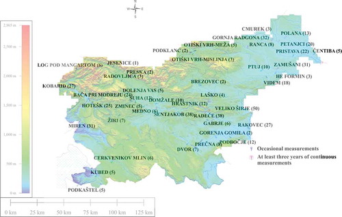
Measurements of suspended solid concentrations and discharges in Slovenia were carried out by the Slovenian Environment Agency (ARSO 2013). Daily time scale datasets were used in this study. The SSC measurements in Slovenia began in 1955. Over more than 50 years of measurements, the network of hydrological monitoring (SSC) gauging stations was modified many times. At most stations, measurements were performed primarily only during high-flow events. Samples of SSC were collected in 1-litre bottles from one point of one vertical of the measuring cross-section, generally between 10 and 20 cm below the water level. In the laboratory, the samples were dried and filtered (Ulaga 2005, Bezak et al. 2013) and eventually SSC concentrations were determined. Figure 1 shows the locations of stations where the monitoring of SSC was performed in the past and a digital elevation model (DEM) of Slovenia. The number of measuring years is given in parentheses, and, in total, more than 500 station-years (not all are complete) of data are available (Fig. 1). A more detailed analysis was performed on the stations that have at least 3 years of continuous daily SSC measurements. These stations have in total more than 300 station-years of data (Bezak et al. 2013). Table 1 shows some basic properties of the analysed catchments and gauging stations that have at least 3 years of daily continuous SSC measurements. Data samples from these stations were analysed in detail. For the Šentjakob (Sava River), Radeče (Sava River) and Veliko Širje (Savinja River) gauging stations, different periods were also examined (Table 1). Continuous daily SSC data are available up to the year 2006; between 2006 and 2012 observations were performed only during high flows, although not all high flows were recorded; and since 2012 SSC monitoring has been interrupted (Bezak et al. 2013). The monitoring is expected to start again at the end of 2015.

Table 1. Basic properties of gauging stations with at least 3 years of continuous SSC measurements.

Station	Stream	Analysed period	Drainage area (km^2)	Mean elevation (m a.s.l.)	Mean daily Q (m^3/s)	Mean daily SSC (g/m^3)	Transported SST (t/year)
Gornja Radgona	Mura	1977–2005	10 197	1012	150.7	49.5	407 388
Petanjci	Mura	1956–1973	10 391	998	171.7	111.0	1 015 948
Polana	Ledava	1963–1973	208	283	1.6	140.7	20 985
Ranca	Pesnica	1967–1973	84	362	1.1	55.1	3 769
Zamušani	Pesnica	1967–1973	478	288	5.8	47.6	15 057
Šentjakob	Sava	1955–1973	2285	931	97.5	23.9	142 775
Šentjakob	Sava	1978–1993	2285	931	84.3	23.8	157 370
Hrastnik	Sava	1997–2006	5177	733	152.7	24.0	241 030
Radeče	Sava	1955–1973	7084	701	232.3	84.1	838 544
Radeče	Sava	1975–1993	7084	701	209.0	69.5	739 304
Laško	Savinja	1990–1993	1664	624	38.7	25.1	98 586
Veliko Širje	Savinja	1955–1973	1842	605	45.6	54.5	167 766
Veliko Širje	Savinja	1978–1989	1842	605	45.3	51.3	216 285
Veliko Širje	Savinja	1994–2005	1842	605	39.9	46.8	216 237
Kobarid	Soča	1962–1973	437	1192	35.1	19.3	52 560
Miren	Vipava	1985–2005	590	153	16.7	19.0	29 785

Figure 1. Locations of gauging stations where SSC measurements were performed on a DEM of Slovenia. Number of measuring years is given in parentheses.

3 Methodology

Altogether, SSC and Q data for 12 gauging stations with different series lengths and periods were analysed in detail (Table 1), meaning that trend, flood frequency, seasonality and lag analyses were performed. All gauging stations have at least 3 years of daily continuous SSC measurements and corresponding Q data. The methodology used to perform analyses is described in the next paragraphs.

Homogeneity and stationarity of the data samples (and the test of potential outliers due to the measurement error) should be tested before the frequency analysis. The Mann-Kendall test (MK; Kendall 1975, Douglas et al. 2000) was used to check whether the sample was stationary, the standard normal homogeneity test (SNHT; Sahin and Cigizoglu 2010) was used to test whether the sample was homogeneous, and the Grubbs test (Grubbs 1950) was applied to determine the potential outliers in the data sample. Successive events must also be independent; however, in the case of the AM series there were usually no problems with autocorrelation in the samples. For peaks over threshold (POT) samples, independence of peaks was ensured using the independence criteria suggested by the Water Resources Council (USWRC 1982):

(1)

where A is the catchment area in square miles, x_S1 and x_S2 are two consecutive peak values, and θ is inter-event duration (time between two successive occurrences of an event; Lang et al. 1999). The second peak should be rejected if one of the conditions in equation (1) is valid.

In the next step, flood frequency analyses were performed for stationary and homogeneous samples that do not contain any potential outliers due to the measurement errors. If a sample contained less than 14 years of data, the POT method was used to define a sample for the frequency analyses. The POT samples, which include, on average, one (POT1), three (POT3) and five (POT5) peaks over the threshold per year were analysed. If a dataset was longer than 14 years, a frequency analysis was carried out with the AM series method. The POT method involved the Poisson distribution for modelling the annual number of events above the threshold and the exponential distribution for the magnitudes of the exceedences. More details about the POT method can be found in Lang et al. (1999), Önöz and Bayazit (2001) and Bezak et al. (2014a). The generalized extreme value (GEV), exponential, Gamma, generalized Pareto, Gumbel, Pearson 3, log-Pearson 3, and log-normal distributions were used with the AM series method (Hosking and Wallis 2005). The parameters of these distributions were estimated with the method of L-moments (Hosking and Wallis 2005). The root mean square error (RMSE), mean absolute error (MAE) and Akaike information criterion (AIC) were used to select the distributions that gave the best fit to the AM series samples (Bezak et al. 2014a). The AIC selection criteria can be calculated with the expression:

(2)

where n is the data sample size, k is the number of distribution parameters, and RMSE is the selection criteria result. In order to evaluate the connection between Q and SSC the Pearson and Kendall correlation coefficients were also calculated for the daily Q and SSC values.

Furthermore, the seasonal behaviour of Q and SSC was also observed. Data were divided based on four seasons: winter (January, February and March), spring (April, May and June), summer (July, August and September) and autumn (October, November and December). For each year, the maximum event (Q and SSC) of each season was determined (seasonal maxima) with the following methodology: seasons with the highest (maximum) and lowest (minimum) 3rd quartile value were selected as those with maximum or minimum Q and SSC values.

The lag between the peak Q and the corresponding maximum SSC was also calculated. First, we defined POT samples of Q with an average of five peaks per year (POT5). Then, the corresponding maximum values of the SSC were determined in the period of 5 days before and after the peak Q event. These analyses were carried out for all gauging stations (Fig. 1). In the case of gauging stations where measurements were not continuous (many times, there was no measurement of SSC around the maximum Q event in the selected period), the peak Q event was withdrawn from the analyses, so only events with both measured variables were selected. For some gauging stations, we could determine only a few events in which both variables (Q and SSC) were observed. The Pearson correlation coefficient between the peak Q and the corresponding maximum SSC was also calculated.

4 Results and discussion

The results and discussion section is divided into four parts. The first part (Section 4.1) shows results for the trends and changes analyses; Section 4.2 shows frequency analysis (Q and SSC) results; Section 4.3 shows results of seasonality and extreme events analyses. These analysis were carried out for gauging stations with at least 3 years of continuous measurements (Table 1) and with less than 1% of missing values (SSC measurements). Section 4.4 shows results for the average lag analysis between the peak Q and the corresponding SSC for all gauging stations (Fig. 1) together with the corresponding Pearson correlation coefficients.

4.1 Analysis of trends and changes

Table 2 shows the Mann-Kendall test results with significance levels for the 11 gauging stations with at least 3 years of continuous SSC measurements. Results for the Laško station are not shown due to the short series (Table 2). The POT1 and the AM samples were used to investigate trends and changes. One can see that no uniform (positive or negative) trend can be found in the analysed data samples (Table 2). Most of the Q series expressed positive trends, but few results were statistically significant (POT1 sample for the Petanjci station on the Gornja Radgona River). For the SSC series, approximately one-half of the samples expressed a negative trend, and the other half, a positive trend. All of the statistically significant trends were decreasing: the AM sample for the Polana station on the Ledava River, the AM and POT1 samples for the Laško station on the Savinja River, the AM sample for the Veliko Širje station on the Savinja River (1955–1973), and the POT1 sample for the Kobarid station on the Soča River. Series with statistically significant trends (negative) were not used for frequency analysis. The reasons for these statistically significant negative trends include the construction of wastewater treatment plants, sedimentation in the accumulation reservoirs of hydropower plants, and closed mines in some regions.

Table 2. Mann-Kendall test results with the corresponding significance levels for the annual maximum (AM) and POT1 selection of Q and SSC samples for stations with at least 3 years of continuous SSC measurements.

Station	Period	AM-Q	POT1-Q	AM-SSC	POT1-SSC
Gornja Radgona	1977–2005	0.38 (29.2)	−0.30 (23.6)	0.36 (27.9)	1.18 (76.3)
Petanjci	1956–1973	1.17 (75.9)	2.31 (97.9)	−1.63 (89.7)	−1.71 (91.2)
Polana	1963–1973	−0.86 (60.8)	−0.23 (18.5)	−2.88 (99.6)	−0.86 (60.8)
Ranca	1967–1973	1.22 (77.6)	1.35 (82.4)	0.15 (11.9)	−1.95 (94.9)
Zamušani	1967–1973	1.05 (70.7)	1.05 (70.7)	−1.52 (87.1)	−1.82 (93.2)
Šentjakob	1955–1973	1.12 (73.7)	−0.28 (22.5)	−0.18 (13.9)	−0.04 (2.8)
Šentjakob	1978–1993	−0.81 (58.2)	−1.89 (94.1)	−1.17 (75.8)	−1.08 (72.0)
Hrastnik	1997–2006	−1.88 (93.9)	−0.27 (21.2)	0.45 (34.5)	1.70 (91.7)
Radeče	1955–1973	1.78 (92.0)	0.74 (53.7)	−0.56 (42.5)	−1.33 (81.7)
Radeče	1975–1993	0.46 (35.7)	0.53 (40.2)	0.53 (40.2)	−0.39 (29.9)
Veliko Širje	1955–1973	0.11 (8.4)	0.77 (55.9)	−2.90 (99.6)	0.11 (8.4)
Veliko Širje	1978–1989	0.96 (66.3)	−0.27 (21.6)	1.51 (86.9)	−0.96 (66.3)
Veliko Širje	1994–2005	−1.51 (86.9)	0.96 (66.3)	−0.69 (50.7)	0.69 (50.7)
Kobarid	1962–1973	−0.76 (55.3)	0.90 (63.1)	−2.88 (99.6)	−2.33 (98.2)
Miren	1985–2005	0.60 (45.4)	1.09 (72.3)	1.57 (88.4)	1.33 (81.6)

Walling and Fang (2003) also investigated trends in suspended sediment load series and did not find a uniform trend at a global scale (Asia, Europe, North America); nevertheless, the majority of the trends were declining. Tramblay et al. (2008) found that the majority of the statistically significant trends in North American rivers (continental scale) were decreasing (except for two rivers). Benkhaled et al. (2014) also discovered negative trends in the SSC series at the basin scale (Algeria), and similar conclusions were made for rivers in Japan (Luo et al. 2013), where negative trends were also generally found. Bonacci and Oskoruš (2010) analysed changes in the SSC values for three hydrological stations in the lower Danube River (Croatia). Negative trends were characteristic of all three gauging stations. The reason for this was the construction of hydropower plants (dams and accumulation reservoirs) in the upper part of the Danube River. We can make the general statement that the worldwide trends were (are) primarily decreasing trends and also all the statistically significant SSC trends in Slovenia were negative.

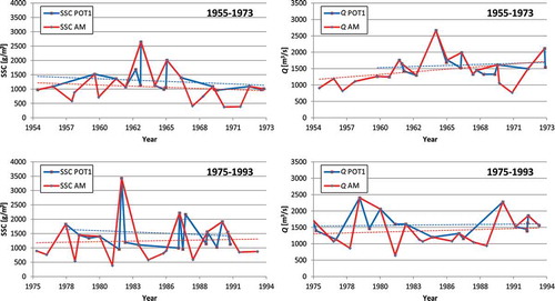
Figure 2 shows the trend results (Q and SSC) for the Radeče station on the Sava River, for two considered periods (1955–1973 and 1975–1993). Dolinar et al. (2008) analysed particle size distribution at different measuring locations near the Radeče station. The AM and POT1 samples with linear trend lines are shown in Fig. 2. Three of the presented SSC samples were negative, but none were statistically significant. However, all of the discharge samples were increasing, but, again, none were statistically significant (Fig. 2). Furthermore, sample selection methodology (POT or AM) clearly has an influence on the trend analysis results independently of the considered variables (Q or SSC; Table 2). Bezak et al. (2014b) investigated the influence of sample selection (AM or POT) on the flood frequency analysis and statistical trend analysis results, and the conclusion was that the data sample selection methodology can have significant influence on the final results. One can see that this is obviously also the case for the Radeče station (period 1975–1993), where the SSC AM sample indicates a positive trend and a negative trend is characteristic of the SSC POT1 sample.

Figure 2. The SSC and Q trends for the Radeče station for two different periods and for two samples.

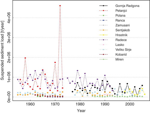
Figure 3 shows annual suspended sediment loads (SST) for all the considered gauging stations with at least 3 years of continuous SSC measurements. The SST values were calculated as a product of Q and SSC (ARSO 2013). One can see that the amount of transported material is generally decreasing. Annual suspended sediment load rates span from 1000 t/year (for the Ranca station on the Pesnica River) to 4.6 × 10⁶ t/year (for the Petanjci station on the Mura River). Diversity in the amounts of transported material is large mostly because catchments with areas from 84 to 10 391 km² were analysed (Table 1).

Figure 3. Annual suspended sediment loads for all stations with at least 3 years of continuous daily SSC measurements.

4.2 Frequency analysis of peaks of discharge and suspended sediment concentration

Before frequency analyses of Q and SSC data were carried out, the MK (Table 2), SNHT and Grubbs tests were conducted in order to ensure that samples are stationary and homogeneous, and do not contain any potential outliers due to measurement error. Table 3 shows selected samples (AM or POT) and the best fit distributions, which were determined with the use of the RMSE, MAE and AIC model selection criteria and a graphical goodness-of-fit test. In the case of the AM samples, there was also no problem with the autocorrelation of the consecutive events; however, for the POT samples, independence of the consecutive events was ensured using independence criteria (equation (1)). All Q samples in Table 3 were homogeneous and stationary with a significance level of 0.01 and did not contain any potential outliers. The same can be said for the SSC samples (Table 3), with the exception of those for the Zamušani gauging station on the Pesnica River, which was non-homogeneous (significance level 0.01) and the Ranca gauging station on the Pesnica River, which contained one potential outlier (19/7/1971; 2260 g/m³); therefore, these two stations were not used for further frequency analysis and are also not shown in Table 3. If the AM sample was non-homogeneous or non-stationary, then the POT sample (POT1, POT3, or POT5) was used instead (e.g. the Veliko Širje gauging station; period 1955–1973). For approximately one-half of the samples, the AM series method was used (Table 3). The Gumbel (or extreme value type I) distribution function gave the best results in 7 of 15 samples. These results were not surprising because extreme events were observed (AM and POT samples). Frequency analyses of peak Q and SSC series were performed on the samples presented in Table 3. Table 4 shows the results of the frequency analysis for return periods of 10 and 100 years. As we can see, there is no relationship between the best fit distribution and the catchment area, length of data series and location of station in the case of Slovenian streams (Table 3); therefore, no generalization is possible for the best fit distribution despite the fact that the Gumbel distribution function was selected as the most appropriate in almost half of the considered AM cases. Similar conclusions were also made by other researchers. For example, Tramblay et al. (2008) performed frequency analysis on suspended sediment concentration data at a continental scale in North America and found that log-normal and exponential distributions gave the best results in most cases (only the AM series method was used), and exponential, log-normal, Weibull and Gamma distributions were used for 90% of the gauging stations. The log-normal distribution also gave the best results for frequency analysis of the SSC series in Algeria (Benkhaled et al. 2014).

Table 3. Selected samples (AM or POT) and the chosen best fit distribution functions for gauging stations in Slovenia with at least 3 years of continuous SSC measurements.

Station	Period	Q		SSC
		Sample	Distribution	Sample	Distribution
Gornja Radgona	1977–2005	AM	Gumbel	AM	Gumbel
Petanjci	1956–1973	AM	Exponential	AM	GEV
Polana	1963–1973	POT3	/	POT3	/
Šentjakob	1955–1973	AM	Pearson 3	AM	Gumbel
Šentjakob	1978–1993	AM	Gumbel	AM	Gumbel
Hrastnik	1997–2006	POT5	/	POT3	/
Radeče	1955–1973	AM	Gumbel	AM	Pearson 3
Radeče	1975–1993	AM	Exponential	AM	Gumbel
Laško	1990–1993	POT5	/	POT5	/
Veliko Širje	1955–1973	AM	GEV	POT1	/
Veliko Širje	1978–1989	POT3	/	POT3	/
Veliko Širje	1994–2005	POT3	/	POT3	/
Kobarid	1962–1973	POT5	/	POT5	/
Miren	1985–2005	AM	Gamma	AM	Exponential

Table 4. Flood frequency analysis results (return periods of 10 and 100 years) for the Q and SSC samples.

		Q		SSC
Station	Period	Q10 (m^3/s)	Q100 (m^3/s)	SSC10 (g/m^3)	SSC100 (g/m^3)
Gornja Radgona	1977–2005	935	1379	1808	2961
Petanjci	1956–1973	1149	1973	3487	12 195
Polana	1963–1973	55	84	5579	8303
Šentjakob	1955–1973	938	1252	928	1420
Šentjakob	1978–1993	984	1474	1309	2114
Hrastnik	1997–2006	1394	2013	1434	2274
Radeče	1955–1973	2101	3016	1823	2723
Radeče	1975–1993	2118	3396	2273	4093
Laško	1990–1993	791	1166	866	1263
Veliko Širje	1955–1973	676	1104	3416	5866
Veliko Širje	1978–1989	713	1042	2326	3444
Veliko Širje	1994–2005	578	831	3303	5070
Kobarid	1962–1973	432	621	753	1150
Miren	1985–2005	270	339	1026	1906

Because different hydrological periods were analysed, it is difficult to compare different stations, despite the fact that some stations are located in the same catchments (Mura, Sava, Savinja). However, the location of the station is not the only parameter that influences SSC values. Pearson correlation coefficients between the catchment area and the mean daily Q and SSC values were 0.88 and 0.30, respectively. This means that the Q values were much more dependent on the size of the catchment area than on the SSC values.

4.3 Seasonality and extreme event analysis of the Q and SSC peaks

The results of the seasonality analysis for gauging stations with at least 3 years of continuous daily SSC measurements are presented in Table 5. Seasons with the highest and lowest 3rd quartile value were selected as those with maximum or minimum Q and SSC values. Therefore, each year of measurements gave four maximum and minimum values, one maximum and one minimum for each season. For stations with shorter dataset lengths, these results, presented in Table 5, can be somewhat less accurate. For the Laško station on the Savinja River, only 4 years were analysed, and only four events were defined in each season (maximum or minimum).

Table 5. Seasons with the highest and lowest values (3rd quartile) of seasonal maxima for the Q and SSC samples.

Station	Period	Q		SSC
		Minimum	Maximum	Minimum	Maximum
Gornja Radgona	1977–2005	Winter	Summer	Winter	Summer
Petanjci	1956–1973	Winter	Summer	Winter	Spring
Polana	1963–1973	Autumn	Summer	Summer	Winter
Ranca	1967–1973	Autumn	Summer	Autumn	Summer
Zamušani	1967–1973	Autumn	Summer	Winter	Spring
Šentjakob	1955–1973	Winter	Autumn	Summer	Winter
Šentjakob	1978–1993	Summer	Autumn	Winter	Autumn
Hrastnik	1997–2006	Winter	Autumn	Winter	Autumn
Radeče	1955–1973	Spring	Autumn	Winter	Summer
Radeče	1975–1993	Spring	Autumn	Spring	Autumn
Laško	1990–1993	Summer	Autumn	Winter	Autumn
Veliko Širje	1955–1973	Winter	Autumn	Winter	Summer
Veliko Širje	1978–1989	Summer	Autumn	Winter	Summer
Veliko Širje	1994–2005	Spring	Autumn	Winter	Autumn
Kobarid	1962–1973	Winter	Autumn	Winter	Summer
Miren	1985–2005	Summer	Autumn	Spring	Autumn

From Table 5 we can see that for most of the analysed data samples (for some stations more samples were analysed), the maximum SSC occurred in summer (short-term intense convective precipitation produced by thunderstorms) or autumn (prolonged frontal precipitation) months, whereas minimum values were characteristic of the winter season. For Q values, most of the maxima occurred in the autumn, and most of the minima occurred in the winter. The alpine pluvial–nival water regime (high flows in autumn and spring; low flows in winter and summer) is characteristic of the Laško, Veliko Širje, Šentjakob, Hrastnik and Radeče stations; the alpine nival–pluvial regime (high flows at the end of spring, at the beginning of summer, and in autumn; low flows in winter) is characteristic of the Gornja Radgona, Petanjci and Kobarid stations; the Panonian pluvial–nival water regime (high flows in spring and autumn; low flows in summer and winter) is characteristic of the Polana, Ranca and Zamušani stations; and the Dinaric pluvial–nival water regime (high flows in spring and autumn; low flows in summer) is characteristic of the Miren station on the Vipava River (Frantar and Hrvatin 2005). Our results are primarily in agreement with typical water regimes of the analysed gauging stations, where most of the low Q and SSC values were measured in the winter and high values were characteristic of the autumn. For some stations, high values of SSC also occurred in the summer. Tramblay et al. (2008) found that most of the SSC maxima occurred in spring and summer (179 stations in North America). Spring peaks were caused by snowmelt and rainfall processes, whereas summer peaks were associated with thunderstorms (high rainfall intensity). Rodríguez-Blanco et al. (2010), Benkhaled et al. (2014) and Guzman et al. (2013) also discovered that the SSC values were not constant during the year. Figure 4 shows seasonal maxima for the Veliko Širje station on the Savinja River for the period of 1955–1973. This station was selected due to the availability of a relatively long series.

Figure 4. Seasonal maxima for the Veliko Širje station on the Savinja River for the period 1955–1973.

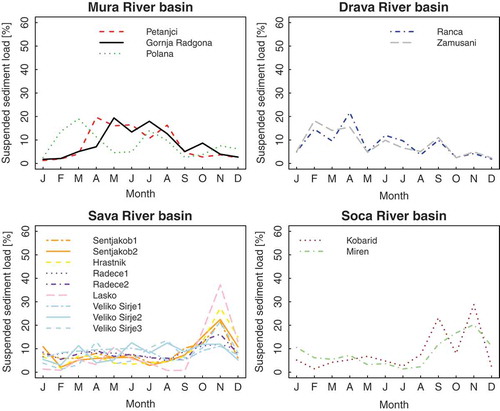
Figure 5 shows percentages of the mean daily suspended sediment loads (SST) carried in particular months for gauging stations with continuous SSC measurements. Stations are grouped based on large river catchments (Mura, Drava, Sava and Soča river basins). For both stations on the Mura River a clear summer peak of the SST is noticeable, whereas for the stations in the Soča and Sava river basins SST peaks usually occurred in autumn. For stations in the Drava River basin the maximum amount of the suspended material was transported in winter. However analysed data series for Ranca and Zamušani stations were relatively short; therefore, the uncertainty connected with the results for these two stations cannot be neglected.

Figure 5. Seasonal behaviour of the suspended sediment loads for stations grouped into four major river catchments.

Due to the fact that linear or exponential functions are often used for the estimation of the SSC values based on the Q values, the correlation coefficients between these two variables were also calculated in order to access the reasonableness of this procedure. Table 6 shows the Kendall correlation coefficients for the Q–SSC values for the gauging stations with at least 3 years of continuous SSC measurements. In our case, suspended sediment load (SST) values were calculated as the product of the Q and SSC values; therefore, the correlation between Q–SST and SSC–SST was not considered. The Kendall correlation coefficient values for the Q–SSC pair were relatively low, from a minimum of 0.01 for the Radeče station on the Sava River to 0.41 for the Gornja Radgona station on the Mura River (Table 6). This means that high (low) Q values do not necessarily mean high (low) SSC values, and the use of Q–SSC curves for estimating unmeasured suspended sediment loads is doubtful. Examples of the use of the Q–SSC curve can be found in Achite and Ouillon (2007), Gilja et al. (2009), Guzman et al. (2013) and Harrington and Harrington (2013). Rodríguez-Blanco et al. (2010) stated that if the scatter between the Q and SSC values is large, then the rating curve method does not seem appropriate to estimate SSC values. Significant scatter in the relationship between Q and SSC can be a consequence of the hysteretic behaviour of the SSC and Q during runoff events and the exhaustion of sediment sources in catchments. This scatter behaviour also indicates that the connection between Q and SSC is not purely hydraulic (Rodríguez-Blanco et al. 2010). Kisi et al. (2008) also found that the use of Q–SSC curves can lead to insufficient results. As an alternative, some authors used neuro-fuzzy and neural networks models (Kisi et al. 2008) and also hysteresis models (Eder et al. 2010). Roman et al. (2012) applied regional regression models and Isik (2013) used regional rating curve models of suspended sediment load to estimate annual suspended sediment loads. Tramblay et al. (2008) found that, for more than half of the considered stations in North America, the correlation between the SSC peak and the corresponding Q peak was statistically significant (Kendall correlation coefficient) at a significance level of 10%.

Table 6. Kendall correlation coefficients for the Q and SSC samples for at least 3 years of SSC continuous measurements.

Station	Period	Q–SSC
Gornja Radgona	1977–2005	0.41
Petanjci	1956–1973	0.36
Polana	1963–1973	0.20
Ranca	1967–1973	0.17
Zamušani	1967–1973	0.38
Šentjakob	1955–1973	0.20
Šentjakob	1978–1993	0.28
Hrastnik	1997–2006	0.26
Radeče	1955–1973	0.01
Radeče	1975–1993	0.12
Laško	1990–1993	0.33
Veliko Širje	1955–1973	0.30
Veliko Širje	1978–1989	0.39
Veliko Širje	1994–2005	0.36
Kobarid	1962–1973	0.29
Miren	1985–2005	0.30

Furthermore, the Pearson correlation coefficients between Q and SSC values for the complete daily series of all stations (including stations with less than 3 years of continuous measurements) were also calculated in order to evaluate the results presented in the previous paragraph. These correlation coefficients varied from 0.05 to 0.59. These results confirm the conclusion made in the previous paragraph that a large scatter is present in the Q–SSC relationship, which can be caused by seasonal, hysteresis and sediment depletion (exhaustion) effects (Moliere et al. 2004). In order to access the connection between the selected geographical characteristics of stations and calculated correlation coefficients between Q and SSC, the Pearson correlation coefficient was calculated again. The Pearson correlation coefficient between the number of years and the Pearson correlation coefficients between Q and SSC was 0.27, with a corresponding p-value of 0.37; however, the Pearson correlation coefficient between the size of the catchment area and the Pearson correlation coefficients between daily Q and SSC values for all gauging stations was 0.41, with a p-value of 0.02. These values indicate that for large catchment areas the correlation was generally larger than for smaller catchments. Nevertheless, there was no connection between station location and the calculated correlation coefficients between Q and SSC. These results also indicate that the relationship between Q and SSC is not purely linear.

In order to confirm or to reject the conclusions from previous paragraphs that Q–SSC curves should be used with caution, we have also investigated the coincidence of the maximum Q event with the maximum SSC event. The date and magnitude of the maximum discharge Q_MAX and the corresponding suspended sediment concentration SSC_COR, and the maximum suspended sediment concentration SSC_MAX and the corresponding discharge Q_COR in the observed period for gauging stations with at least 3 years of continuous measurements are presented in Table 7. For all considered gauging stations shown in Table 7, a different event was selected as the maximum (Q_MAX and SSC_MAX). These can be understood as confirmation of the assumption that the use of Q–SSC curves can be questionable. Extreme discharge events are not necessarily extreme suspended sediment load events. The results shown in Table 7 should be used with care because in the case of extreme events (floods), it is occasionally difficult to capture a representative sample; however, significant variability in Q–SSC cannot be rejected. Rodríguez-Blanco et al. (2010) found that higher water yields did not necessarily occur in the same months as high suspended sediment load values, which can be interpreted in the same way as the results presented in this study.

Table 7. Maximum (Q_MAX and SSC_MAX) and corresponding (SSC_COR and Q_COR) values and dates in the observed period for the selected stations.

Station	Period	Date	QMAX (m^3/s)	SSCCOR (g/m^3)	Date	SSCMAX (g/m^3)	QCOR (m^3/s)
Gornja Radgona	1977–2005	22/8/2005	1236	1247	16/5/1996	2364	464
Petanjci	1956–1973	17/7/1972	1251	896	22/4/1972	8770	936
Polana	1963–1973	15/7/1972	68	823	17/3/1963	9621	7
Ranca	1967–1973	25/9/1973	31	26	19/7/1971	2260	0.5
Zamušani	1967–1973	16/7/1972	142	62	6/9/1967	517	3
Šentjakob	1955–1973	5/11/1966	1046	351	8/6/1956	1121	105
Šentjakob	1978–1993	29/1/1979	1100	311	14/11/1982	1363	1051
Hrastnik	1997–2006	5/11/1998	1473	424	6/12/2005	3341	683
Radeče	1955–1973	25/10/1964	2670	790	15/8/1963	2647	150
Radeče	1975–1993	29/1/1979	2403	1450	25/7/1982	3426	153
Laško	1990–1993	1/11/1990	826	329	26/11/1990	1255	149
Veliko Širje	1955–1973	25/9/1973	925	18	28/10/1959	9303	9
Veliko Širje	1978–1989	9/10/1980	911	847	9/8/1989	2790	246
Veliko Širje	1994–2005	5/11/1998	1037	2228	14/4/1994	9574	147
Kobarid	1962–1973	14/11/1969	475	190	8/9/1962	1032	211
Miren	1985–2005	5/11/1998	298	67	27/10/2004	1105	13

4.4 Analysis of the lag between peak discharges and the corresponding concentrations

The average lag between peak Q (POT5) and the corresponding maximum SSC value in the period of 5 days before and 5 days after the peak discharge were also analysed. Figure 6 shows the results of this analysis for stations with more than 20 complete events, when there were both Q and SSC values available. Positive lag values (solid fill) mean that the corresponding SSC maximum on average occurred before the peak Q values defined with the POT5 sample. The pattern fill denotes the opposite situation, and circles with no fill denote cases where there was no lag between the observed variables (on average). The number of analysed events is written in brackets (Fig. 6).

Figure 6. Average lag values between peak Q values defined as the POT5 sample and the corresponding maximum values of SSC.

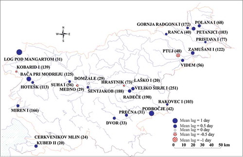
For most of the stations, the corresponding SSC peaks on average occurred before peak Q (Fig. 6). For these stations, most of the suspended sediment load originated from the stream channel itself. For stations in which the peak Q on average occurred before the corresponding SSC, this could mean that the main erosion areas are more distant from streams. The timing of Q and SSC peaks is dependent on different factors, such as the distance of erosion areas from the streams, bank erosion, hillslope processes (Lenzi and Marchi 2000, Mao and Lenzi 2007) and erosion of a channel. Tramblay et al. (2010b) analysed the average lag between SSC peaks and the corresponding Q peaks in the period of 3 days before and after the SSC peak. In the case of small catchments, the SSC peak usually occurred before the Q peak, and in most cases the time difference was small, which was also the case for most of the Slovenian streams (Fig. 6). Average lag values can also be compared with the clockwise (positive) and counterclockwise (negative) hysteretic loops, which indicate two distinct cases: the first indicates the case in which the maximum SSC value occurs before the peak Q, and the second indicates the opposite situation (Gellis 2013). Soler et al. (2008) analysed two adjacent catchments in the Mediterranean area and concluded that positive loops were characteristic of large events (precipitation, runoff, peak Q); in contrast, negative loops were typical for small events. Smith and Dragovich (2009) also found that the SSC peak primarily occurred before the peak Q (clockwise hysteresis loops). For more reliable conclusions, measurements with more precise time steps (e.g. hourly) should be carried out. In our study also no regional pattern can be found in the results presented in Fig. 6. The Pearson correlation coefficient value between the average lag value and the basin catchment area was −0.24. This means that the size of the catchment area does not have a major influence on the average lag values in the case of data from the Slovenian streams. The Pearson correlation coefficient value between the number of events and the mean lag values was 0.08. From this, we can conclude that the number of events does not have any influence on the average lag results. Similarly, no connection between the location of stations and the mean lag values could be found.

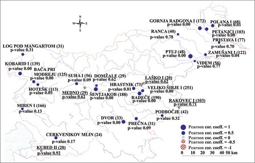
In the next step we also analysed the connection between the peak Q and the corresponding SSC maxima in the period of 5 days before or 5 days after the peak Q event by calculating the Pearson correlation coefficient between the peak Q and the corresponding SSC values. The correlation coefficient values and p-values are presented in Fig. 7. If the p-value is smaller than the chosen significance level (0.01 or 0.05), one can reject the null hypothesis (H₀: there is no correlation between variables) and accept the alternative hypothesis (H_A: variables are linearly correlated; negatively or positively) with a chosen probability error (the number of considered events is an important factor). In the case of four gauging stations, the Pearson correlation coefficient values were negative (names of the stations underlined in Fig. 7: Kubed, Medno, Laško and Rakovec) with significance levels larger than 0.05. For 13 stations, the p-values were less than or equal to the chosen significance level of 0.05, which means the peak Q values and the corresponding SSC peaks are linearly correlated (at the chosen significance level). Furthermore, no geographical pattern could be found in the results presented in Fig. 7.

Figure 7. Pearson correlation coefficient values between peak Q and the corresponding maximum values of SSC.

5 Conclusions

In total more than 500 station-years of daily SSC, Q and SST data from Slovenian streams measured with direct sampling methods were used for the analyses, which were performed at a national scale. Trends, changes, seasonality, lag and frequency analyses were performed on data measured at stations with catchment areas of between 100 and 10 000 km². The following conclusions may be drawn from this study:

1. The trend analysis for the SSC samples at a national scale indicates that approximately-half of the samples expressed a negative trend, and the other half, a positive trend. Nevertheless, all the statistically significant trends were decreasing. Some possible reasons for the statistically significant negative trends include the construction of wastewater treatment plants, sedimentation in the accumulation reservoirs of hydropower plants and closed mines in some regions.

2. For gauging stations with at least 3 years of continuous daily SSC measurements, frequency analyses, which are not often performed, were carried out (Q and SSC samples). No generalization is possible for the best fit distribution in the case of the AM samples (Table 3); however, the Gumbel distribution gave the best results according to the RMSE, MAE and AIC models selection criteria and graphical goodness-of-fit test in almost half of the considered AM samples. Furthermore, differences among some distributions were not significant, meaning that some other distribution function could be selected in some cases.

3. A seasonality analysis showed that the characteristics of the considered data samples were primarily in agreement with the water regimes of stations (Table 5). Most of the peaks occurred in the summer (thunderstorms) and autumn (frontal precipitation), whereas deficits were primarily characteristic of winter. In one-half of the analysed samples the maximum (3rd quartile value) of Q coincided with the SSC maximum of the 3rd quartile value (Table 5). Furthermore, the Kendall correlation coefficients between Q and SSC were relatively small (for stations shown in Table 1), meaning that scatter between variables is not negligibly small (Table 6), and also the maximum Q event did not coincide with the maximum SSC event (Table 7) for gauging stations with at least 3 years of continuous daily SSC measurements (Table 1). These indicate that Q–SSC curves should be used with caution.

4. For most of the stations, the peak Q on average occurred after the corresponding SSC maximum (Fig. 6), which is primarily the case for small catchments (clockwise-positive hysteresis loops). The mean time differences were quite small—less than 1 day; however, one should keep in mind that daily observations were used for calculations of these mean lag values. No connection between the mean lag values and the catchment area was found (Pearson correlation coefficient: −0.24). No geographical pattern could be found in the average lag values (Fig. 6) and the corresponding correlation coefficient values (Fig. 7).

The results of the study indicate that, despite the fact that all of the statistically significant trends in the SSC series in Slovenian streams were negative, continuous measurements of this variable are still needed, because continuous series are a precondition for performing SSC frequency analysis, which yields a relationship between design variable and recurrence interval that is often used in practical applications. Furthermore, surrogate methods would probably be more appropriate than direct sampling methods, which were used for gathering data analysed in this study, because measurements with a more precise time step are more easily obtained than in the case of direct sampling methods. Due to the low correlation between Q and SSC values, rating curve models are probably not an optimal choice for the estimation of the missing SSC values. Furthermore, maximum Q events were usually not coincident with the maximum SSC events, meaning that making SSC measurements only during high-flow events is not an optimal solution, because the maximum SSC values can occur at other times of the year than the maximum Q event (despite the well-known fact that most of the suspended material is transported during a few extreme events, some suspended sediment load can be overlooked) and also lag analyses showed that peak Q on average occurred after the corresponding SSC maximum. All these analyses show that continuous observations of the SSC variable are necessary.

Acknowledgements

We wish to thank the Environmental Agency of the Republic of Slovenia for data provision and Florjana Ulaga for detailed explanations of the measurement of suspended sediment loads in Slovenia.

Disclosure statement

No potential conflict of interest was reported by the authors.

Additional information

Funding

The results of the study are part of the UL FGG work on the international research project SedAlp, which is financed by the European Union through the Alpine Space programme. The research was also partially financially supported by the Slovenian Research Agency through the PhD grant of the first author (N. Bezak).

References

- Achite, M. and Ouillon, S., 2007. Suspended sediment transport in a semiarid watershed, Wadi Abd, Algeria (1973–1995). Journal of Hydrology, 343 (3–4), 187–202. doi:10.1016/j.jhydrol.2007.06.026
- ARSO. 2013. ARSO. http://vode.arso.gov.si/hidarhiv/pov_arhiv_tab.php. [Accessed 27 August 2013].
- Benkhaled, A., et al., 2014. Frequency analysis of annual maximum suspended sediment concentrations in Abiod wadi, Biskra (Algeria). Hydrological Processes, 28, 3841–3854. doi:10.1002/hyp.9880.
- Bezak, N., Brilly, M., and Šraj, M., 2014a. Comparison between the peaks-over-threshold method and the annual maximum method for flood frequency analysis. Hydrological Sciences Journal, 59 (5), 959–977. doi:10.1080/02626667.2013.831174
- Bezak, N., Brilly, M., and Šraj, M., 2014b. Flood frequency analyses, statistical trends and seasonality analyses of discharge data: a case study of the Litija station on the Sava River. Journal of Flood Risk Management. doi:10.1111/jfr3.12118.
- Bezak, N., Šraj, M., and Mikoš, M., 2013. Overview of suspended sediments measurements in Slovenia and an example of data analysis. Gradbeni Vestnik, 62, 274–280. (In Slovenian).
- Bilotta, G.S. and Brazier, R.E., 2008. Understanding the influence of suspended solids on water quality and aquatic biota. Water Research, 42 (12), 2849–2861. doi:10.1016/j.watres.2008.03.018
- Bonacci, O. and Oskoruš, D., 2010. The changes in the lower Drava River water level, discharge and suspended sediment regime. Environmental Earth Sciences, 59 (8), 1661–1670. doi:10.1007/s12665-009-0148-8
- Dolinar, B., Vrecl-Kojc, H., and Trauner, L., 2008. Analysis of concentration and sedimentation of suspended load in the reservoirs. Acta Geotechnica Slovenica, 5 (2), 41–49.
- Douglas, E.M., Vogel, R.M., and Kroll, C.N., 2000. Trends in floods and low flows in the United States: impact of spatial correlation. Journal of Hydrology, 240 (1–2), 90–105. doi:10.1016/S0022-1694(00)00336-X
- Eder, A., et al., 2010. Comparative calculation of suspended sediment loads with respect to hysteresis effects (in the Petzenkirchen catchment, Austria). Journal of Hydrology, 389 (1–2), 168–176. doi:10.1016/j.jhydrol.2010.05.043
- Frantar, P. and Hrvatin, M., 2005. Pretocni rezimi v Sloveniji med letoma 1971 in 2000. Geografski Vestnik, 77, 115–127.
- Gellis, A.C., 2013. Factors influencing storm-generated suspended-sediment concentrations and loads in four basins of contrasting land use, humid-tropical Puerto Rico. Catena, 104, 39–57. doi:10.1016/j.catena.2012.10.018
- Gilja, G., Bekic, D., and Oskorus, D. 2009. Processing of suspended sediment concentration measurements on Drava River. In: P. Cvetanka, J. Milorad, eds. Eleventh international symposium on water management and hydraulic engineering, 1–5 September, Skopje. 181–191. ISBN: 978-9989-2469-6-8
- Gray, J.R. and Gartner, J.W., 2009. Technological advances in suspended-sediment surrogate monitoring. Water Resources Research, 45, 20. doi:10.1029/2008WR007063
- Grubbs, F.E., 1950. Sample criteria for testing outlying observations. The Annals of Mathematical Statistics, 21 (1), 27–58. doi:10.1214/aoms/1177729885
- Guzman, C.D., et al., 2013. Suspended sediment concentration-discharge relationships in the (sub-) humid Ethiopian highlands. Hydrology and Earth System Sciences, 17 (3), 1067–1077. doi:10.5194/hess-17-1067-2013
- Harrington, S.T. and Harrington, J.R., 2013. An assessment of the suspended sediment rating curve approach for load estimation on the Rivers Bandon and Owenabue, Ireland. Geomorphology, 185, 27–38. doi:10.1016/j.geomorph.2012.12.002
- Higgins, H., et al., 2011. Suspended sediment dynamics in a tributary of the Saint John River, New Brunswick. Canadian Journal of Civil Engineering, 38 (2), 221–232. doi:10.1139/L10-129
- Hosking, J.R.M. and Wallis, J.R., 2005. Regional frequency analysis: an approach based on L-moments. Cambridge: Cambridge University Press.
- Isik, S., 2013. Regional rating curve models of suspended sediment transport for Turkey. Earth Science Informatics, 6 (2), 87–98. doi:10.1007/s12145-013-0113-7
- Kendall, M.G., 1975. Multivariate analysis. London: Griffin.
- Khoi, D.N. and Suetsugi, T., 2014. Impact of climate and land-use changes on hydrological processes and sediment yield—a case study of the be River catchment, Vietnam. Hydrological Sciences Journal, 59 (5), 1095–1108. doi:10.1080/02626667.2013.819433
- Kisi, O., Yuksel, I., and Dogan, E., 2008. Modelling daily suspended sediment of rivers in Turkey using several data-driven techniques / Modélisation de la charge journalière en matières en suspension dans des rivières turques à l’aide de plusieurs techniques empiriques. Hydrological Sciences Journal, 53 (6), 1270–1285. doi:10.1623/hysj.53.6.1270
- Lang, M., Ouarda, T., and Bobée, B., 1999. Towards operational guidelines for over-threshold modeling. Journal of Hydrology, 225 (3–4), 103–117. doi:10.1016/S0022-1694(99)00167-5
- Lenzi, M.A., Mao, L., and Comiti, F., 2003. Interannual variation of suspended sediment load and sediment yield in an alpine catchment. Hydrological Sciences Journal, 48 (6), 899–915. doi:10.1623/hysj.48.6.899.51425
- Lenzi, M.A. and Marchi, L., 2000. Suspended sediment load during floods in a small stream of the Dolomites (northeastern Italy). Catena, 39 (4), 267–282. doi:10.1016/S0341-8162(00)00079-5
- López-Tarazón, J.A., et al., 2009. Suspended sediment transport in a highly erodible catchment: the River Isábena (Southern Pyrenees). Geomorphology, 109 (3–4), 210–221. doi:10.1016/j.geomorph.2009.03.003
- López-Tarazón, J.A., et al., 2010. Rainfall, runoff and sediment transport relations in a mesoscale mountainous catchment: the River Isábena (Ebro basin). Catena, 82 (1), 23–34. doi:10.1016/j.catena.2010.04.005
- Luo, P.P., et al., 2013. Statistical analysis and estimation of annual suspended sediments of major rivers in Japan. Environmental Science: Processes & Impacts, 15 (5), 1052–1061. doi:10.1039/c3em30777h
- Mao, L. and Lenzi, M.A., 2007. Sediment mobility and bedload transport conditions in an alpine stream. Hydrological Processes, 21 (14), 1882–1891. doi:10.1002/hyp.6372
- Moliere, D.R., et al., 2004. Estimation of suspended sediment loads in a seasonal stream in the wet-dry tropics, Northern Territory, Australia. Hydrological Processes, 18, 531–544. doi:10.1002/hyp.1336
- Nourani, V., Kalantari, O., and Baghanam, A.H., 2012. Two semidistributed ANN-based models for estimation of suspended sediment load. Journal of Hydrologic Engineering, 17 (12), 1368–1380. doi:10.1061/(ASCE)HE.1943-5584.0000587
- Önöz, B. and Bayazit, M., 2001. Effect of the occurrence process of the peaks over threshold on the flood estimates. Journal of Hydrology, 244 (1–2), 86–96. doi:10.1016/S0022-1694(01)00330-4
- Rodríguez-Blanco, M.L., et al., 2010. Temporal changes in suspended sediment transport in an Atlantic catchment, NW Spain. Geomorphology, 123 (1–2), 181–188. doi:10.1016/j.geomorph.2010.07.015
- Roman, D.C., Vogel, R.M., and Schwarz, G.E., 2012. Regional regression models of watershed suspended-sediment discharge for the eastern United States. Journal of Hydrology, 472–473, 53–62. doi:10.1016/j.jhydrol.2012.09.011
- Rusjan, S., Brilly, M., and Mikoš, M., 2008. Flushing of nitrate from a forested watershed: an insight into hydrological nitrate mobilization mechanisms through seasonal high-frequency stream nitrate dynamics. Journal of Hydrology, 354 (1–4), 187–202. doi:10.1016/j.jhydrol.2008.03.009
- Sahin, S. and Cigizoglu, H.K., 2010. Homogeneity analysis of Turkish meteorological data set. Hydrological Processes, 24 (8), 981–992. doi:10.1002/hyp.7534
- Simon, A. and Klimetz, L., 2008. Magnitude, frequency, and duration relations for suspended sediment in stable (“Reference”) Southeastern streams. JAWRA Journal of the American Water Resources Association, 44 (5), 1270–1283. doi:10.1111/j.1752-1688.2008.00222.x
- Smith, H.G. and Dragovich, D., 2009. Interpreting sediment delivery processes using suspended sediment-discharge hysteresis patterns from nested upland catchments, south-eastern Australia. Hydrological Processes, 23 (17), 2415–2426. doi:10.1002/hyp.7357
- Soler, M., Latron, J., and Gallart, F., 2008. Relationships between suspended sediment concentrations and discharge in two small research basins in a mountainous Mediterranean area (Vallcebre, Eastern Pyrenees). Geomorphology, 98 (1–2), 143–152. doi:10.1016/j.geomorph.2007.02.032
- Tena, A., et al., 2011. Suspended sediment dynamics in a large regulated river over a 10-year period (the lower Ebro, NE Iberian Peninsula). Geomorphology, 125 (1), 73–84. doi:10.1016/j.geomorph.2010.07.029
- Tramblay, Y., et al., 2010a. Regional estimation of extreme suspended sediment concentrations using watershed characteristics. Journal of Hydrology, 380 (3–4), 305–317. doi:10.1016/j.jhydrol.2009.11.006
- Tramblay, Y., et al., 2010b. Estimation of local extreme suspended sediment concentrations in California Rivers. Science of the Total Environment, 408 (19), 4221–4229. doi:10.1016/j.scitotenv.2010.05.001
- Tramblay, Y., St-Hilaire, A., and Ouarda, T., 2008. Frequency analysis of maximum annual suspended sediment concentrations in North America / Analyse fréquentielle des maximums annuels de concentration en sédiments en suspension en Amérique du Nord. Hydrological Sciences Journal, 53 (1), 236–252. doi:10.1623/hysj.53.1.236
- Ulaga, F., 2005. Monitoring suspendiranega materiala v slovenskih rekah (Monitoring of suspended matter in Slovenian rivers in Slovenian). Acta Hydrotechnica, 23, 117–127.
- USWRC (United States. Interagency Advisory Committee on Water Data. Hydrology Subcommittee), 1982. Guidelines for determining flood flow frequency. Reston, VA: US Department of the Interior, Geological Survey, Office of Water Data Coordination.
- Walling, D.E., 1999. Linking land use, erosion and sediment yields in river basins. Hydrobiologia, 410, 223–240. doi:10.1023/A:1003825813091
- Walling, D.E., 2005. Tracing suspended sediment sources in catchments and river systems. Science of the Total Environment, 344 (1–3), 159–184. doi:10.1016/j.scitotenv.2005.02.011
- Walling, D.E., Collins, A.L., and Stroud, R.W., 2008. Tracing suspended sediment and particulate phosphorus sources in catchments. Journal of Hydrology, 350 (3–4), 274–289. doi:10.1016/j.jhydrol.2007.10.047
- Walling, D.E. and Fang, D., 2003. Recent trends in the suspended sediment loads of the world’s rivers. Global and Planetary Change, 39 (1–2), 111–126. doi:10.1016/S0921-8181(03)00020-1
- Wren, D.G., et al., 2000. Field techniques for suspended-sediment measurement. Journal of Hydraulic Engineering-ASCE, 126 (2), 97–104. doi:10.1061/(ASCE)0733-9429(2000)126:2(97)