Climate change impacts on groundwater hydrology – where are the main uncertainties and can they be reduced?

ABSTRACT

This paper assesses how various sources of uncertainty propagate through the uncertainty cascade from emission scenarios through climate models and hydrological models to impacts, with a particular focus on groundwater aspects from a number of coordinated studies in Denmark. Our results are similar to those from surface water studies showing that climate model uncertainty dominates the results for projections of climate change impacts on streamflow and groundwater heads. However, we found uncertainties related to geological conceptualization and hydrological model discretization to be dominant for projections of well field capture zones, while the climate model uncertainty here is of minor importance. How to reduce the uncertainties on climate change impact projections related to groundwater is discussed, with an emphasis on the potential for reducing climate model biases through the use of fully coupled climate–hydrology models.

Editor D. Koutsoyiannis; Associate editor not assigned

KEYWORDS:

• climate change
• hydrological change
• uncertainty cascade
• groundwater
• coupled climate–hydrology model

1 Introduction

Numerous studies of climate change impacts on hydrology have been presented during the past decade (Bates et al. 2008, Jiménez Cisneros et al. 2014). The present climate projections exhibit large uncertainties arising from assumptions on greenhouse gas emissions, incomplete climate models and initial conditions (Hawkins and Sutton 2009, 2011, IPCC 2013). When assessing climate change impacts on groundwater and surface water, uncertainties related to downscaling or bias correction of climate data and uncertainties in hydrological models must also be addressed. The key sources of uncertainty related to hydrological models originate from data, parameter values and model structure (Refsgaard et al. 2007). The model structural uncertainty includes aspects related to process equations, conceptualization of the local hydrological system being studied, spatial and temporal discretization and numerical approximations. For groundwater models, conceptualizations of the geology often constitute a major source of (model structural) uncertainty (Bredehoeft 2005, Refsgaard et al. 2012). As uncertainties from the “upstream” sources propagate through the chain of calculations (greenhouse gas emission scenarios → general circulation models (GCMs) → regional climate models (RCMs) → downscaling/bias correction methods → hydrological models → hydrological impacts), the complete suite of uncertainties has been referred to as the uncertainty cascade (Foley 2010, Refsgaard et al. 2012).

Several studies have assessed uncertainty propagation through parts of the cascade using Monte Carlo techniques (Bastola et al. 2011, Poulin et al. 2011, Dobler et al. 2012, Velázquez et al. 2013, Vansteenkiste et al. 2014). The complexities and computational aspects involved prevent inclusion of all sources of uncertainty in any one study, and we are not aware of a study where uncertainties originating from all sources in the uncertainty cascade from emission scenarios to hydrological change have been quantified. Few studies have attempted to include more than a couple of uncertainty sources in one analysis. Wilby and Harris (2006) used information from two emission scenarios, two GCMs, two downscaling methods, two hydrological model structures and two sets of hydrological model parameters for assessing uncertainties in climate change impacts on low flows in the UK. Using a similar probabilistic approach, Chen et al. (2011) combined results from an ensemble of two emission scenarios, five GCMs, five GCM initial conditions, four downscaling methods, three hydrological model structures and 10 sets of hydrological model parameters for studying uncertainties in climate change impacts on streamflows in Canada.

As uncertainties related to climate projections are often considerable (Jiménez Cisneros et al. 2014), many stakeholders and policy makers may, at a first glance, be scared of the propagation and addition of new uncertainties through the uncertainty cascade, where it may be perceived that uncertainties will increase dramatically. The impacts of the different sources of uncertainties on the resulting hydrological change uncertainty are, however, context specific (Refsgaard et al. 2013). Most studies have found that uncertainty related to climate models was more important than hydrological model structure uncertainty (Wilby and Harris 2006, Chen et al. 2011, Dobler et al. 2012), while some studies found hydrological model structures to be equally important, in particular for low-flow simulations (Bastola et al. 2011, Velázquez et al. 2013). Similarly, in a study on groundwater well field capture zones, Sonnenborg et al. (2015) found that the uncertainty at a “downstream” point (geology) in the calculation chain dominated, making the effects of climate model uncertainty negligible.

Since it is not feasible to make calculations for the entire uncertainty cascade, and since the dominating sources of uncertainty are context specific, there is a need for guidance on which sources of uncertainty to include in a specific hydrological impact uncertainty assessment. Useful guidance related to river runoff can be found in e.g. Wilby and Harris (2006), Chen et al. (2011) and Bastola et al. (2011). Many fewer studies have been performed for groundwater aspects, and, to our knowledge, no guidance exists on the relative importance of the various sources of uncertainty affecting climate change impacts on groundwater.

The large uncertainties on the hydrological impacts render the results not easily applicable in practical water management, where climate change adaptation decisions require more accuracy than is often possible with today’s knowledge and modelling tools. Kundzewicz and Stakhiv (2010) argued that climate models, because of their large inherent uncertainties, are not ready for water resources management applications, while Wilby (2010) argued that relatively little is known about the significance of climate model uncertainty. Depending on the nature of the sources of uncertainty, strategies to deal with uncertainty in climate change adaptation may vary from reducing the uncertainty by gaining more knowledge (epistemic uncertainty) to living with the uncertainty that is non-reducible (aleatory uncertainty) (Refsgaard et al. 2013). In this respect it is interesting to evaluate which sources of uncertainty in the uncertainty cascade could potentially be reduced.

As climate models are acknowledged to reproduce observed climate data with significant biases (Anagnostopoulos et al. 2010, Huard 2011, Koutsoyiannis et al. 2011, Boberg and Christensen 2012, Seaby et al. 2015), the prospects for improving climate models are particularly relevant. The current climate models have several recognized weaknesses, e.g. related to descriptions of atmospheric processes and spatio-temporal resolutions (Kendon et al. 2014, Stevens and Bony 2013, Rummukainen et al. 2015). In the present paper, however, we limit our analysis to the hydrologically relevant interaction between land surface and atmosphere. Climate models include only a simplistic description of land surface and subsurface processes, and, similarly, hydrological models generally only include atmospheric processes in a surface-near layer on the scale of metres. Proper representation of land surface conditions is recognized as being crucial for describing the energy balance of the land–atmosphere interaction (Sellers and Hall 1992). It can therefore be hypothesized that a fully coupled climate–hydrology model with a more comprehensive and complete description of subsurface processes, instead of simplified parameterizations or ignorance of processes (i.e. subsurface lateral flow of water and connection with deeper aquifers), could reduce the bias and hence the uncertainty of climate and hydrological change projections. Several research groups are therefore experimenting with various concepts of fully coupled models. Zabel and Mauser (2013) showed results from the 76 665 km² Upper Danube catchment in Central Europe using a coupling between the hydrological land surface model PROMET and the regional climate model MM5. Goodall et al. (2013) established a technically sophisticated coupling between the SWAT surface water hydrological model and the Earth System Modelling Framework. In order to include the feedback from groundwater systems, Maxwell et al. (2007), Kollet and Maxwell (2008), Rihani et al. (2010) and Maxwell et al. (2011) established a number of couplings between the ParFlow hydrological model, land surface models (CLM, Noah) and atmospheric models (ARPS, WRF), while Butts et al. (2014) established a coupling between the regional climate model HIRHAM and the MIKE SHE hydrological model code.

The objectives of the present paper are (i) to assess the relative importance of the different sources in the uncertainty cascade in climate change impact projections with focus on groundwater; and (ii) to evaluate the prospects for reducing uncertainty in groundwater impact projections.

2 Methodology

The present paper analyses results from a large number of recently published studies on climate change impacts on groundwater in Denmark. These studies each focussed on individual aspects, while here we synthesize the findings into an uncertainty cascade framework, discussing them in an international state-of-the-art context. In order to complete the analysis, we also present one new analysis.

Comparison of results from the different studies is facilitated by common approaches, as explained below.

2.1 Uncertainty cascade

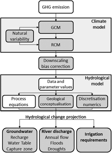
The uncertainty cascade from emission scenarios to hydrological change projections is illustrated in Figure 1, where the topics shown in shaded boxes are illustrated by a synthesis of results from the Danish studies, while the elements in unshaded boxes are only discussed based on international literature. Overall, the approach has been to address some key sources of uncertainty both in climate modelling and in hydrological modelling, and quantify them in a variety of cases with different contexts. The key reasons to give priority to many different test cases rather than a more comprehensive uncertainty analysis for a single case, like Wilby and Harris (2006) and Chen et al. (2011), are: (i) we want to analyse how different sources of uncertainty dominate for different model projection purposes and for different hydrological regimes; and (ii) some of the elements that we do not address, such as uncertainty of hydrological parameter values, have been extensively studied previously.

Figure 1. The uncertainty cascade from emission scenarios to hydrological change projections. The elements for which results from the Danish studies are shown in the paper are shaded.

2.2 Study sites and site-specific purposes

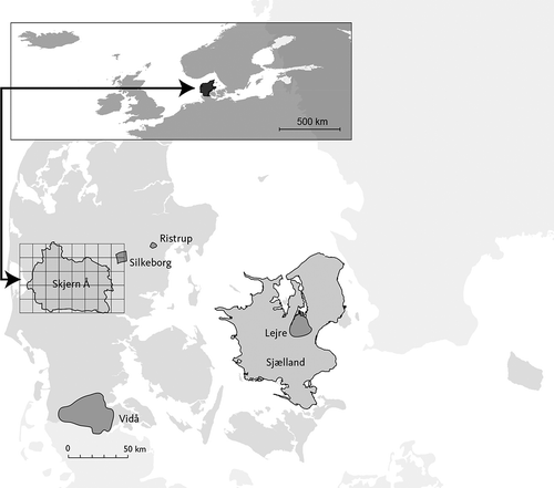
Table 1 provides an overview of the studies carried out, highlighting the context, variables of interest and sources of uncertainty included. The locations of the Danish study sites are shown in Figure 2. The international study site was the FIFE area in Kansas, USA.

Table 1. Overview of studies addressing uncertainties at different steps in the uncertainty cascade.

Case/purpose	Catchment area	Variables of interest	Uncertainty sources	Reference
Inherent variability in climate model	Denmark (43 000 km^2)	Seasonal precipitation	Climate variability	Larsen et al. (2013)
Inherent variability in climate model	FIFE, Kansas, USA (15 km × 15 km)	Daily precipitation	Climate variability	Rasmussen et al. (2012b)
Land surface–atmosphere fluxes	FIFE, Kansas, USA (15 km × 15 km)	Precipitation, temperature, humidity, wind speed, radiation	Feedbacks between climate models and hydrological models	Larsen et al. (2016c)
Land surface–atmosphere fluxes	Skjern Å catchment (2500 km^2)	Precipitation, temperature, humidity, wind speed, radiation	Feedbacks between climate models and hydrological models	Butts et al. (2014), Larsen et al. (2014)
Future precipitation 2011–2100	Denmark (43 000 km^2)	Annual precipitation Extreme precipitation	Climate models Bias correction	Seaby et al. (2013)
National climate adaptation planning 2021–2050	Denmark (43 000 km^2)	Groundwater level (average, min, max) Discharge (average, min, max)	Climate models Parameter uncertainty	Henriksen et al. (2012)
Future hydrology 2071–2100	Sjælland (7200 km^2)	Groundwater level (average, min, max) Discharge (average, min, max)	Climate models Bias correction	Seaby et al. (2015)
Water resources impact 2071–2100	Vidaa catchment (850 km^2)	Irrigation requirements Low flow	Bias correction	Rasmussen et al. (2012a)
Motorway, design and construction 2081–2100	Silkeborg (103 km^2 – nested into larger model)	Extreme groundwater levels	Climate variability Climate models Bias correction	Kidmose et al. (2013)
Water works, water supply 2071–2100	Lejre (465 km^2)	Discharge groundwater levels Well field capture zone	Climate models Hydrological model structure (geology)	Seifert et al. (2012), Sonnenborg et al. (2015)
Well field, water supply 2081–2100	Ristrup (18.4 km^2 – nested into larger model)	Groundwater level drawdown when abstracting groundwater	Climate models Hydrological model structure (discretization, resolution)	Vilhelmsen (2012)

FIFE: First International Satellite Land Surface Climatological Project Field Experiment .

Figure 2. Location of study sites in Denmark and the extent of the HIRHAM domain covering northern Europe.

2.3 Climate modelling

The analyses of climate modelling uncertainty were based on results from the ENSEMBLE-based Predictions of Climate Changes and their Impacts (ENSEMBLES) project (van der Linden and Mitchell 2009), which ran multiple pairings of GCMs and RCMs for climate projections using the A1B emission scenario. For the present study, a subset of 11 climate models (GCM-RCM pairings) with 25 km resolution and projections to the end of the 21st century were selected from the ENSEMBLES matrix (Seaby et al. 2013).

Climate systems show a strong element of natural variability. Therefore, different plausible initial or boundary conditions for climate models may result in significantly different climate projection pathways (Hawkins and Sutton 2009). This inherent natural climate variability was analysed using different configurations of RCMs in terms of domain sizes and spatial grid resolution for WRF over the USA (Rasmussen et al. 2012b) and for HIRHAM over Denmark (Larsen et al. 2013). In addition, experiments were made with perturbations of the initial conditions in a coupled HIRHAM–MIKE SHE model covering part of Denmark (Larsen et al. 2014). Finally, extreme value analyses reflecting natural climate variability were presented for a study of extreme groundwater levels in Silkeborg, Denmark (Kidmose et al. 2013).

2.4 Statistical downscaling and bias correction of climate model output

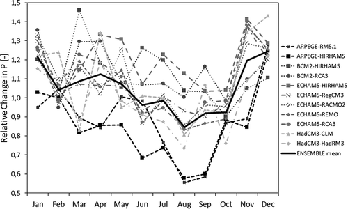
Daily data for the period 1951–2100 on precipitation, temperature and the variables required for performing Penman calculations of reference evapotranspiration (radiation, temperature, wind speed and relative humidity) were downloaded from the ENSEMBLES database and converted from the 25 km RCM grids to the 10 km grid used by Danish Meteorological Institute in its gridded product of observed precipitation (Seaby et al. 2013). The raw data from the RCMs were compared with observed data for 1991–2010 (reference period) for precipitation, temperature and reference evapotranspiration. To reduce substantial biases, two different correction methods were initially applied: (i) the traditional delta change method (DC) with monthly change factors (Fig. 3) reflecting the differences in climate model projections between the reference period and the future study period (Hay et al. 2000); and (ii) a distribution-based scaling (DBS) for precipitation using double Gamma distributions for the lower 95% and the upper 5% of the data (Piani et al. 2010) supplemented with a simple bias removal for temperature and reference evapotranspiration applied on a seasonal basis. These two methods were used on six different domains covering Denmark (43 000 km²) resulting in a set of change and scaling factors, each representing one of the six domains (Seaby et al. 2013). While preserving a zero overall bias for each domain, the DBS-corrected precipitation data turned out to inherit a considerable spatial bias within each of the six domains, and two additional DBS-based methods were therefore introduced for precipitation data: (iii) DBS with scaling in six domains across the country supplemented by a grid-by-grid removal of the bias in average precipitation; and (iv) DBS scaling of precipitation on a 10 km grid basis. Thus, altogether four bias correction methods were tested for precipitation (Seaby et al. 2015).

Figure 3. Monthly delta change factors for precipitation projections for Denmark for 2071–2100 compared to the 1991–2010 reference period for 11 climate models. Figure from Seaby et al. (2013). Reprinted with permission from Elsevier.

2.5 Hydrological impact modelling

The hydrological modelling was in most cases based on coupled groundwater–surface water modelling using the MIKE SHE code with 3D groundwater, 1D unsaturated zone including an evapotranspiration routine, 1D river routing and 2D overland flow modules, enabling direct use of the bias-corrected climate model output as forcing data for the hydrological model. The models were in all cases autocalibrated using PEST (Doherty 2010). In one case a pure MODFLOW-based groundwater model was used (Vilhelmsen 2012), but here the groundwater recharge input was calculated with the Danish national water resources model (Henriksen et al. 2003) using MIKE SHE.

Two specific model structure-related sources of uncertainty were examined in two different cases:

1. Geological conceptualization was studied by establishing six hydrological models based on six different geological conceptualizations but otherwise identical (Seifert et al. 2012).

2. The influence of numerical discretization and geological resolution on simulations of groundwater flow was studied by using a regional model having a 500 m grid and two models with locally refined 100 m grids but different with respect to geological resolution (Vilhelmsen 2012).

2.6 Coupled HIRHAM–MIKE SHE model

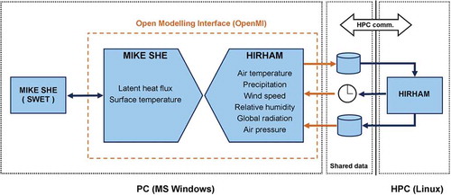
The coupling concept is illustrated schematically in Figure 4. The two model codes can only be executed on different software platforms, Linux and MS Windows, which technically is a substantial complication described in detail by Butts et al. (2014). The coupled model was tested on the 2500 km² groundwater-dominated Skjern River catchment (Larsen et al. 2014). The model domains for HIRHAM and MIKE SHE are shown in Figure 2. HIRHAM was run for a 2800 km × 4000 km domain, while MIKE SHE was confined to the 2500 km² catchment. Outside the Skjern River catchment HIRHAM used its own land surface scheme, which then was replaced by the MIKE SHE coupling within the catchment. HIRHAM operated with a time step of 2 minutes, while the basic time step in MIKE SHE was 1 hour. Various coupling intervals for exchange of data between the two models were analysed, concluding that a 30-minute data exchange interval provides a good trade-off between accuracy and computational demand (Larsen et al. 2014). The coupled model was run for a 1-year period with additional spin-up periods of 3 months for HIRHAM and MIKE SHE’s unsaturated zone and several years for the saturated zone.

Figure 4. Schematic of the HIRHAM–MIKE SHE coupling. Both model codes have been extended with OpenMI Linkable Components, exposing selected variables to each other within the OpenMI platform. The MIKE SHE code runs on the same PC (MS Windows) as the OpenMI software, whereas the HIRHAM code runs on a massively parallelized Cray XT5 high-performance computer system (HPC). Linking directly to the HPC is not possible, necessitating data exchange by files and introducing a considerable overhead in simulations. Figure from Butts et al. (2014). Reprinted with permission from Elsevier.

3 Results and discussion

3.1 Emission scenarios

The studies listed in Table 1 do not include evaluations of alternative emission scenarios. Other studies have concluded that the uncertainty due to unknown future emissions can be considered small compared to climate model uncertainty and natural variability for the coming decades (Wilby and Harris 2006, Chen et al. 2011, Hawkins and Sutton 2011), while the importance at the end of the century (Hawkins and Sutton 2011) and for high-end CO₂ emissions (Karlsson et al. 2015) may be significant.

As the actual future emissions result from human decisions, reduction of uncertainties on emissions is beyond a natural science analysis.

3.2 Climate modelling

3.2.1 GCMs and RCMs and coupled climate–hydrology models

Seaby et al. (2013, 2015) showed that climate model uncertainty is substantial, in particular for precipitation, as illustrated in Figure 3. This finding is in line with international literature (Wilby and Harris 2006, Chen et al. 2011), where uncertainties related to GCM/RCMs often constitute the dominating source compared to bias correction methods and hydrological impact models. The same conclusion has been reached for streamflow and groundwater heads in Denmark (Seaby et al. 2015, Karlsson et al. 2016).

Each climate model has its own set of biases (Seaby et al. 2015). Bias correction methods can remove the biases when calibrated against observations from the present climate. However, as the climate model biases in projected climates are expected to be different from the biases in the present climate, the bias correction methods will likely only be able to reduce, but not to fully remove, climate model biases for projected future climates (Teutchbein and Seibert 2013, Seaby et al. 2015). As these biases of projected future climates cannot be known, the bias correction methods contribute substantially to the impact uncertainty. Based on tests of four bias correction methods for 11 climate models, Seaby et al. (2015) suggest that the bias corrections are more robust the smaller the biases are. So, altogether the climate model uncertainty will be reduced if the basic model biases are reduced.

Significant improvements in modelling approaches and improved confidence in precipitation projections have been seen recently, due, amongst other factors, to higher resolution in space and time (Kendon et al. 2014). In addition, the potential of using coupled models to improve the land surface–atmosphere description of water and energy fluxes is obvious (Maxwell and Kollet 2008). The establishment of a fully coupled, operational HIRHAM–MIKE SHE model (Fig. 4) (Butts et al. 2014, Larsen et al. 2014) opens up the possibility to analyse whether a coupled model is able to reduce the biases of a regional climate model.

While Zabel and Mauser (2013) found that biases were reduced when using a fully coupled model, Larsen et al. (2014) found that results from the coupled HIRHAM-MIKE SHE for a 1-year period have similar or slightly larger biases than results from HIRHAM stand-alone for many of the standard meteorological variables, i.e. precipitation, air temperature, wind speed, relative humidity, radiation and atmospheric pressure. This implies that substituting HIRHAM’s land surface scheme by MIKE SHE does not in itself reduce all biases, even if MIKE SHE has a spatially and physically much more detailed process description of the land surface processes which has been calibrated against field data (Larsen et al. 2016b). While at a first glance this may seem discouraging, it is quite logical. HIRHAM has, over the years, been adjusted to perform better against observational data, and the HIRHAM set-up used in the present coupling was selected from eight model set-ups with different domain coverage and spatial resolution as the one with the smallest overall bias in precipitation (Larsen et al. 2013). Graham and Jacob (2000) reported a similar case, where replacing the land surface scheme in an RCM with a hydrological model resulted in poorer performance of streamflow simulation due to compensational errors in the various components of the RCM. A similar explanation may apply in our case, where the calibrated MIKE SHE model inevitably calculates different energy and water fluxes compared to the HIRHAM land surface scheme it is replacing. As this is the case, a recalibration of the coupled HIRHAM–MIKE SHE model may be required in order to produce simulations with smaller biases. Such simulations are quite similar to what was realized when the first major efforts toward fully coupled atmosphere–ocean models were made. For many years, a flux correction technique had to be applied in order to keep the coupled model system in balance, preventing it from drifting into a model state looking not much like the real world, while each component alone would seem to perform reasonably (Somerville et al. 2007).

Previous coupling studies have either been confined to surface water hydrological models (Goodall et al. 2013, Zabel and Mauser 2013) or, in the case of inclusion of groundwater, been limited to relatively small domains (up to a few hundred km²) and short periods (a few days) for both the climate and the hydrological models (Maxwell et al. 2007, 2011, Kollet and Maxwell 2008, Rihani et al. 2010). In this respect, the Danish results (Butts et al. 2014, Larsen et al. 2014) are novel by including an integrated groundwater–surface water hydrological model in the coupled climate–hydrology model simulation over a long period (more than a year) and a large area (2800 km × 4000 km for the RCM and 2500 km² for the hydrological model). In a follow-up study Larsen et al. (2016a) found, on the basis of a 7-year simulation, that the coupled HIRHAM–MIKE SHE model performed significantly better than the HIRHAM model with respect to simulation of precipitation.

3.2.2 Natural variability – inherent climate model uncertainty

From analyses of multiple set-ups of HIRHAM and WRF over the USA, Rasmussen et al. (2012b) found that the RCM predictions show a high degree of randomness in the precise location of precipitation events at length scales below 130 km, while Larsen et al. (2013) found that HIRHAM showed significantly reduced spatial precision for ranges less than 70 km for monthly precipitation over Denmark. Finally, using the coupled HIRHAM–MIKE SHE model, Larsen et al. (2014) showed that for a full year (1 July 2009 to 30 June 2010) up to 10% differences were found in simulated catchment precipitation among eight model runs that were identical except for different starting dates (between 1 and 8 March 2009). These results clearly reflect the inherent uncertainties in regional-scale climate processes treated in climate models.

Kidmose et al. (2013) performed extreme value analyses to infer maximum groundwater levels with recurrence intervals of 50 and 100 years (T₅₀, T₁₀₀ events) for climate conditions 2081–2100, using nine climate models, two bias correction methods and a hydrological model. Furthermore, they assessed the uncertainties on the extreme events originating from climate models, bias correction and natural variability (confidence intervals in statistical predictions of extreme events using the Gumbel distribution to extrapolate from the 20-year data series to T₅₀ and T₁₀₀ events). They found that natural climate variability constituted between 60% and 75% of the total prediction uncertainties, while the climate model uncertainty contributed between 20% and 35%, and the bias correction methods around 5% (Fig. 5).

Figure 5. Uncertainty on estimation of future extreme groundwater levels originating from climate models, bias correction methods and natural climate variability (extreme value analysis). The curves relate to the absolute values in m (left axis) while the background colours refer to the relative contributions (right axis). Figure modified from Kidmose et al. (2013) © Author(s) 2013. This work is distributedunder the Creative Commons Attribution 3.0 License.

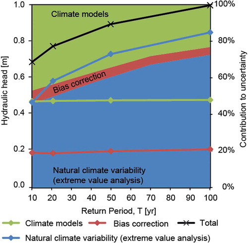
In an analysis of uncertainties in projected decadal mean precipitation over Europe, Hawkins and Sutton (2011) concluded that uncertainty originating from inherent climate variability is of the same order of magnitude as climate model uncertainty, while the effect of using different greenhouse gas (GHG) emission scenarios is negligible. Natural climate variability is known to decrease with increasing spatial and temporal scales of aggregation (Hawkins and Sutton 2011, Rasmussen et al. 2012b, Larsen et al. 2013). Hence, the findings of Kidmose et al. (2013) showing that natural climate variability is twice as large as climate model uncertainty for very small temporal (extreme events) and spatial scales are well in line with previous findings in the literature on this matter.

As the natural variability often dominates over other sources of uncertainty for climate change impact projections in the next few decades, it is interesting to evaluate the potential for reducing the variability. The inherent climate model uncertainty that is often assumed equivalent to the natural climate variability originates from uncertainty on climate model initialization. In this respect, Hawkins and Sutton (2009) note that, while the contribution from internal variability is not reducible far ahead, proper initialization of climate models with observational data should enable some reduction of this uncertainty for the next decade or so. Along the same lines, Olsson et al. (2011) discussed the possibility of reducing this uncertainty by initializing a GCM so that it generates inter-annual variability in phase with historical periods.

3.3 Statistical downscaling and bias correction

Seaby et al. (2015) applied several bias correction methods and propagated the uncertainty from both climate models and bias correction methods through the Danish national water resources model, and inferred the contributions from these two sources of uncertainty on projected groundwater heads and streamflows for Sjælland (Fig. 2). They found that the climate model uncertainty is by far the more important, and that the bias correction methods only explain around 10% of the total uncertainty. They concluded that bias correction contributes relatively more to uncertainty on precipitation than to hydrological uncertainties, and relatively more to uncertainty on extreme events than to values that are averaged over time and space. This finding is well in line with Kidmose et al. (2013), who found climate model uncertainty to be about five times larger than bias correction uncertainty for extreme groundwater events at local scale, as well as with van Roosmalen et al. (2011), who found that two different bias correction methods, DC and DBS, showed only marginal differences for projections of average groundwater levels. Our findings also support Dobler et al. (2012), who concluded that bias correction has the largest influence on projections of extreme events.

A fundamental difference between the DC and the DBS bias correction methods is that DC operates with change factors on the observed climate data, while DBS scales the output from climate models, implying that projected changes in the structure of e.g. precipitation regime in terms of changes in length of dry periods and variations between years is only reflected in the second method. This difference turned out to have significant importance in a study by Rasmussen et al. (2012a), who used one climate model and the two bias correction methods to assess the changes in irrigation requirements for 2071–2100. They found that irrigation will be significantly underestimated when using the DC method due to its inability to account for changes in inter-annual variability in precipitation and reference evapotranspiration.

Uncertainty reduction in bias correction and statistical downscaling deals with developing and selecting accurate and robust methods. A fundamental assumption in statistical downscaling of climate model projections is that the climate model biases are stationary (Refsgaard et al. 2014). Teutschbein and Seibert (2013) applied a differential split-sample test (Klemes 1986) to evaluate different bias correction methods. They found that the simpler correction methods, such as the DC method, are less robust to a non-stationary bias compared to more advanced correction methods. On the other hand, Seaby et al. (2015) found that if bias correction methods are overparameterized they may be less robust in climate conditions different from the reference period for which they were fitted, and that this problem increases the larger the initial bias in the climate model.

3.4 Hydrological impact modelling

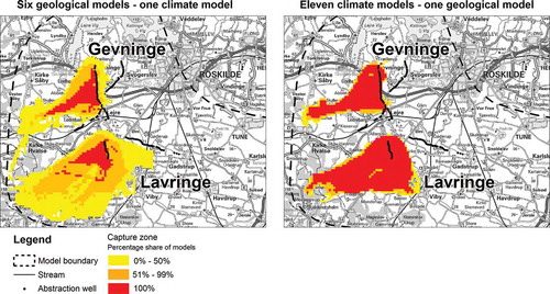
Refsgaard et al. (2012) provided a review of strategies to deal with geologically related uncertainties in hydrological modelling. One of the strategies, to use multiple geological interpretations, was pursued by Seifert et al. (2012), who established six alternative geological conceptualizations for a 465 km² well field area around Lejre (Fig. 2) and calibrated six hydrological models against the same groundwater head and streamflow data series using PEST. The calibration results showed similar overall performance for the six models, where some models were better than others for streamflow but worse for groundwater head simulations, and vice versa, while none of the models were superior to the others in all aspects. The six models were then used for projections of hydrological change due to climate change for the period 2071–2100 (Sonnenborg et al. 2015). Figure 6 shows the climate change impacts on groundwater heads averaged over the period and over the well field area. From this figure it is evident that the spread between climate models is larger than the spread between geological models, and that the differences between geological models become more important the larger the climate change. Analyses of streamflow (not shown here) reveal similar results, namely that the climate model uncertainty dominates geological uncertainty. Figure 7 shows projections of well field capture zones when using six geological models and one climate model (left) and one geology and eleven climate models (right). This shows that the climate model uncertainty has negligible impacts on the capture zone location, while the geological uncertainty clearly dominates, i.e. the opposite of that for groundwater heads and streamflow.

Figure 6. Projected change in mean groundwater level in well field area for 11 climate model projections for 2071–2100. The six lines correspond to the six hydrological models with the corresponding six geological models. Figure based on results from Sonnenborg et al. (2015).

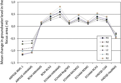
Figure 7. Impacts of geological uncertainty and climate model uncertainty on the location of well field capture zones. The colour indicates percentage of shared capture zones. The figure to the left shows the degree of intersection between projections of six geological/hydrological models using the same climate model. The figure to the right shows the degree of intersection between 11 climate model projections using one geological/hydrological model. Figure from Sonnenborg et al. (2015). © Author(s) 2015. This work is distributedunder the Creative Commons Attribution 3.0 License.

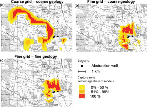
For the present paper, we made a similar analysis for the Ristrup well field (Fig. 2), which pumps from a complex network of buried valleys eroded into low-permeable sediments. Deep aquifers fill the buried valleys, while shallow aquifers are found on the plateaus. The analysis was made using three model set-ups: a regional-scale groundwater model with a 500 m × 500 m grid (coarse grid – coarse geology), and two locally refined groundwater models having 100 m × 100 m grids embedded into the regional model. One of the locally refined models also has a refined geological resolution in the vicinity of the well field (fine grid – fine geology), while the other (fine grid – coarse geology) has the same geological resolution as the regional model (Vilhelmsen 2012). The three models were calibrated against groundwater head time series data covering a 6-year period (1996–2001) and subsequently used to project changes in groundwater heads due to climate change by using recharge series estimated from the same 11 climate models applied by Sonnenborg et al. (2015). Figure 8 shows the relative change in head elevations caused by the different climate models for each of the three groundwater models. Similar to Sonnenborg et al. (2015), we find that the uncertainty in projected heads explained by the climate model exceeds the uncertainties explained by the choice of discretization in groundwater models. However, when projecting the capture zones from a well field located in one of the buried valleys (Fig. 9), we find that the difference between capture zones caused by difference in numerical grid resolution dominates over the difference in capture zones caused by geological resolution, while the smallest difference in capture zones is caused by the choice of climate model input.

Figure 8. Mean relative change in head using recharge data from 11 climate models. The lines indicate simulations with three groundwater models having different numerical and geological resolution.

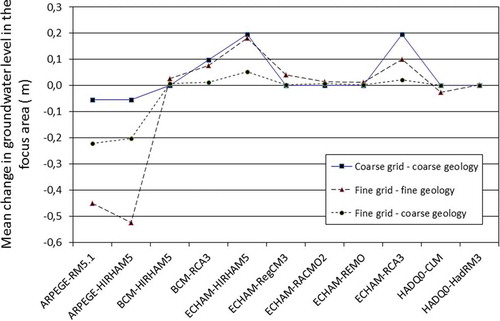
Figure 9. Impacts of numerical and geological resolution compared to climate model uncertainty when projecting well field capture zones. The colours indicate percentages of shared capture zones between climate models for (a) the regional-scale groundwater model, (b) the model with locally refined numerical grid but coarse geological resolution, and (c) the locally refined model also having refined geological resolution.

The importance of site-specific conditions on the uncertainty propagation was evident in a national study of climate change impacts on groundwater levels and extreme river discharge (T₁₀₀), where Henriksen et al. (2012) found significant regional patterns. For example, some regions show small climate change impacts, including small uncertainties, on groundwater heads but large impacts and uncertainties on river discharge, while other regions show the opposite. These differences may be explained by differences in hydrogeological regimes such as confined/unconfined aquifers and degree of tile drainage (Henriksen et al. 2012).

The above findings nicely supplement the international literature confirming that uncertainties in climate change impacts on streamflow are dominated by climate modelling uncertainty. The above Danish studies did not assess the uncertainty due to model structures (process equations) and parameter values of the hydrological models. The impacts of these sources of uncertainty on streamflow projections have, in international studies, been evaluated in general to also be smaller than climate model uncertainty (Wilby and Harris 2006, Bastola et al. 2011, Chen et al. 2011, Dobler et al. 2012). Furthermore, Bastola et al. (2011) and Velázquez et al. (2013) found that hydrological model structure uncertainty in some cases was substantial, while Wilby and Harris (2006) and Poulin et al. (2011) found that model structure uncertainty was more important than parameter uncertainty. The novelty of the Danish studies lies in their focus on geological uncertainty and groundwater, illustrating that the dominating sources of uncertainties are context specific.

Reduction of uncertainties related to hydrological impact modelling is, in general, possible by collecting additional high-quality data and, in some cases, also by enhancing the modelling techniques used (Refsgaard et al. 2007).

4 Conclusions

Through a number of coordinated studies with climate projections towards the end of the present century, we have assessed the uncertainties originating at different points in the chain of calculations (the uncertainty cascade) between greenhouse gas (GHG) emissions and hydrological change, and analysed how various uncertainties are amplified or reduced in their downstream propagation towards hydrological change. For the variable of principal interest in hydrological studies, precipitation, we found that the two dominating climate-related sources of uncertainty are the natural climate variability and the climate models. Both of these sources are much larger than the uncertainties related to GHG emissions found in other studies (van Roosmalen et al. 2007, Hawkins and Sutton 2011) and much larger than the uncertainties related to bias correction methods (Dobler et al. 2012, Kidmose et al. 2013, Seaby et al. 2013). In addition, uncertainties related to the hydrological model are important. Complementary to other studies focussing on model structure (process equations) uncertainty and parameter uncertainty (Wilby and Harris 2006, Bastola et al. 2011, Poulin et al. 2011, Velázquez et al. 2013) we have analysed the impacts of geological uncertainty and alternative model discretization. In one case study (Sonnenborg et al. 2015) we showed that climate model uncertainty dominates over geological uncertainty for projections of streamflow and groundwater heads, while the impacts of geological uncertainty increase with increasing climate change. The same case study showed, however, that geological uncertainty dominates over climate model uncertainty for projections of well field capture zone. This illustrates that the various uncertainties will propagate differently for different projection variables, and in some cases a large climate uncertainty will have negligible impact. We found similar results for another case (Vilhelmsen 2012) where different numerical and geological models were used. Again, climate model uncertainty dominated over groundwater model uncertainty when projecting the mean change in head, whereas the numerical resolution of the groundwater model and, to a lesser degree, its geological resolution were the dominant contributors to the uncertainty when projecting well field capture zones.

Overall, we can conclude that no generic ranking of the relative importance of the sources of uncertainty can be found. The ranking will be context specific depending on the projection variable and the hydrogeological regime. Having said that, we also need to emphasize that there is robust evidence that natural climate variability and climate model uncertainty often dominate for groundwater variables. The exception we found, i.e. that uncertainties on geological conceptualization and numerical discretization overrule climate model uncertainty for projections of groundwater flow paths and well field capture zones, may have some generic validity, but as no other studies reported in the literature have dealt with this issue, we only have evidence from our own two case studies in Denmark to support such a suggestion.

The uncertainties on impact projections are so large that, in practice, they constrain climate change adaptation (Kundzewicz and Stakhiv 2010). Hence, there is an urgent need for reducing uncertainties. This can be done in the traditional way of collecting more high-quality data and using better techniques for bias correction and impact modelling. However, as the largest uncertainty in most cases relates to climate modelling, emphasis should be given to reducing biases in climate models. In addition to the improvement of the climate models themselves (Kendon et al. 2014, Stevens and Bony 2013, Rummukainen et al. 2015), there is considerable potential for reducing uncertainties by applying fully coupled climate–hydrology models such as HIRHAM–MIKE SHE (Butts et al. 2014). Fully coupled models have now proven their capability to carry out comprehensive experiments, which are needed to fully evaluate to what extent their potential will materialize. A recent follow-up study by Larsen et al. (2016b) showing significantly more accurate precipitation simulations with the coupled model is very encouraging in this respect.

Acknowledgements

We are thankful to Jens Asger Andersen (Danish Nature Agency, now at Orbicon), Jørn-Ole Andreasen (Aarhus Water), Troels Kærgaard Bjerre (VCS Denmark), Michelle Kappel (Greater Copenhagen Utility), Dirk-Ingmar Müller-Wohlfeil (Danish Nature Agency) and Mads O. Rasmussen (DHI-GRAS) for providing data, ideas and comments for the Danish studies.

Disclosure statement

No potential conflict of interest was reported by the authors.

Additional information

Funding

The present study was partly funded by a grant from the Danish Strategic Research Council for the project HYdrological Modelling for Assessing Climate Change Impacts at differeNT Scales (HYACINTS, www.hyacints.dk) under contract no. DSF-EnMi 2104-07-0008.

References

- Anagnostopoulos, G.G., et al., 2010. A comparison of local and aggregated climate model outputs with observed data. Hydrological Sciences Journal, 55 (7), 1094–1110. doi:10.1080/02626667.2010.513518
- Bastola, S., Murphy, C., and Sweeney, J., 2011. The role of hydrological modelling uncertainties in climate change impact assessments of Irish river catchments. Advances in Water Resources, 34, 562–576. doi:10.1016/j.advwatres.2011.01.008
- Bates, B.C., et al., eds., 2008. Climate change and water. Technical Paper of the Intergovernmental Panel on Climate Change, IPCC Secretariat, Geneva.
- Boberg, F. and Christensen, J.H., 2012. Overestimation of Mediterranean summer temperature projections due to model deficiencies. Nature Climate Change, 2, 433–436. doi:10.1038/nclimate1454
- Bredehoeft, J., 2005. The conceptualization model problem - surprise. Hydrogeology Journal, 13 (1), 37–46. doi:10.1007/s10040-004-0430-5
- Butts, M., et al., 2014. Embedding complex hydrology in the regional system climate system – dynamic coupling across different modelling domains. Advances in Water Resources, 74, 166–184. doi:10.1016/j.advwatres.2014.09.004
- Chen, J., et al., 2011. Overall uncertainty study of the hydrological impacts of climate change for a Canadian watershed. Water Resources Research, 47, W12509. doi:10.1029/2011WR010602
- Dobler, C., et al., 2012. Quantifying different sources of uncertainty in hydrological projections in an alpine watershed. Hydrology and Earth System Sciences, 16, 4343–4360. doi:10.5194/hess-16-4343-2012
- Doherty, J., 2010. PEST, model-independent parameter estimation, user manual. 5th ed. Australia: Watermark Numerical Computing.
- Foley, A.M., 2010. Uncertainty in regional climate modelling: A review. Progress in Physical Geography, 34 (5), 647–670. doi:10.1177/0309133310375654
- Goodall, J.L., et al., 2013. Coupling climate and hydrological models: interoperability through web services. Environmental Modelling & Software, 46, 250–259. doi:10.1016/j.envsoft.2013.03.019
- Graham, L.P. and Jacob, D., 2000. Using large-scale hydrologic modelling to review runoff generation processes in GCM climate models. Meteorologische Zeitschrift/Contribution to Atmospheric Physics, 1 (1), 43–51.
- Hawkins, E. and Sutton, R., 2009. The potential to narrow uncertainty in regional climate predictions. Bulletin of the American Meteorological Society, 90, 1095–1107. doi:10.1175/2009BAMS2607.1
- Hawkins, E. and Sutton, R., 2011. The potential to narrow uncertainty in projections of regional precipitation change. Climate Dynamics, 37, 407–418. doi:10.1007/s00382-010-0810-6
- Hay, L.E., Wilby, R.J.L., and Leavesley, G.H., 2000. A comparison of delta change and downscaled GCM scenarios for three mountainous basins in the United States. Journal of the American Water Resources Association, 36 (2), 387–397. doi:10.1111/j.1752-1688.2000.tb04276.x
- Henriksen, H.J., et al., 2012. Klimaeffekter på hydrologi og grundvand (Klimagrundvandskort). GEUS Rapport 2012/116 (In Danish). Available from: http://www.klimatilpasning.dk/media/340310/klimagrundvandskort.pdf [Accessed 3 November 2015].
- Henriksen, H.J., et al., 2003. Methodology for construction, calibration and validation of a national hydrological model for Denmark. Journal of Hydrology, 280, 52–71. doi:10.1016/S0022-1694(03)00186-0
- Huard, D., 2011. A black eye for the Hydrological Sciences Journal. Discussion of “A comparison of local and aggregated climate model outputs with observed data” by G.G. Anagnostopoulos et al. (2010) Hydrological Sciences Journal 55(7),1094-1110. Hydrological Sciences Journal, 56 (7), 1330–1333. doi:10.1080/02626667.2011.610758
- IPCC, 2013. Climate change 2013: The physical science basis. Contribution of Working Group I to the Fifth Assessment Report of the Intergovernmental Panel on Climate Change [Stocker, T. F., D. Qin, G.-K. Plattner, M. Tignor, S. K. Allen, J. Boschung, A. Nauels, Y. Xia, V. Bex and P. M. Midgley (eds.)]. Cambridge University Press, Cambridge, United Kingdom and New York, NY, USA, 1535 pp.
- Jiménez Cisneros, B.E., et al., 2014. Freshwater resources. In: Climate Change 2014: Impacts, Adaptation, and Vulnerability. Part A: Global and Sectoral Aspects. Contribution of Working Group II to the Fifth Assessment Report of the Intergovernmental Panel on Climate Change [Field, C.B., Barros, V.R., Dokken, D.J., Mach, K.J., Mastrandrea, M.D., Bilir, T.E., Chatterjee, M., Ebi, K.L., Estrada, Y.O., Genova, R.C., Girma, B., Kissel, E.S., Levy, A.N., MacCracken, S., Mastrandrea, P.R. and White, L.L. (eds.)]. Cambridge University Press, Cambridge, UK and New York, NY, pp. 229–269.
- Karlsson, I.B., et al., 2016. Combined effects of climate models, hydrological model structures and land use scenarios on hydrological impacts of climate change. Journal of Hydrology, 535, 301–317. doi:10.1016/j.jhydrol.2016.01.069
- Karlsson, I.B., et al., 2015. Effect of a high-end CO2-emission scenario on hydrology. Climate Research, 64, 39–54. doi:10.3354/cr01265
- Kendon, E.J., et al., 2014. Heavier summer downpours with climate change revealed by weather forecast resolution model. Nature Climate Change, 4 (7), 570–576. doi:10.1038/nclimate2258
- Kidmose, J., et al., 2013. Climate change impact on groundwater levels: ensemble modelling of extreme values. Hydrology and Earth System Sciences, 17, 1619–1634. doi:10.5194/hess-17-1619-2013
- Klemes, V., 1986. Operational testing of hydrological simulation models. Hydrological Sciences Journal, 31, 13–24. doi:10.1080/02626668609491024
- Kollet, S.J. and Maxwell, R.M., 2008. Capturing the influence of groundwater dynamics on land surface processes using an integrated, distributed watershed model. Water Resources Research, 44, W02402. doi:10.1029/2007WR006004
- Koutsoyiannis, D., et al., 2011. Scientific dialogue on climate: is it giving black eyes or opening closed eyes? Reply to “A black eye for the Hydrological Sciences Journal” by D. Huard. Hydrological Sciences Journal, 56 (7), 1334–1339. doi:10.1080/02626667.2011.610759
- Kundzewicz, Z.W. and Stakhiv, E.Z., 2010. Are climate models “ready for prime time” in water resources management applications, or is more research needed?. Hydrological Sciences Journal, 55 (7), 1085–1089. doi:10.1080/02626667.2010.513211
- Larsen, M.A.D., et al., 2016a. Calibration of a distributed hydrology and land surface model using energy flux measurement. Agricultural and Forest Meteorology, 217, 74–88. http://dx.doi.org/10.1016/j.agrformet.2015.11.012
- Larsen, M.A.D., et al., 2016b. Local control on precipitation in a fully coupled climate-hydrology model. Scientific Reports, 6, 22927. doi:10.1038/srep22927
- Larsen, M.A.D., et al., 2016c. Assessing the influence of groundwater and land surface scheme in the modelling of land surface-atmosphere feedbacks over the FIFE area in Kansas, USA. Environmental Earth Sciences, 75, 130. doi:10.1007/s12665-015-4919-0
- Larsen, M.A.D., et al., 2014. Results from a full coupling of the HIRHAM regional climate model and the MIKE SHE hydrological model for a Danish catchment. Hydrology and Earth System Sciences, 18, 4733–4749. doi:10.5194/hess-18-4733-2014
- Larsen, M.A.D., et al., 2013. On the role of domain size and resolution in the simulations with the HIRHAM region climate model. Climate Dynamics, 40, 2903–2918. doi:10.1007/s00382-012-1513-y
- Maxwell, R.M., Chow, F.K., and Kollet, S.J., 2007. The groundwater-land-surface-atmosphere connection: soil moisture effects on atmospheric boundary layer in fully-coupled simulations. Advances in Water Resources, 30, 2447–2466. doi:10.1016/j.advwatres.2007.05.018
- Maxwell, R.M. and Kollet, S.J., 2008. Interdependence of groundwater dynamics and land-energy feedbacks under climate change. Nature Geoscience, 1 (10), 665–669. doi:10.1038/ngeo315
- Maxwell, R.M., et al., 2011. Development of a coupled groundwater-atmosphere model. Monthly Weather Review, 39, 96–116. doi:10.1175/2010MWR3392.1
- Olsson, J., et al., 2011. Using an ensemble of climate projections for simulating recent and near-future hydrological change to lake Vänern in Sweden. Tellus, 63A, 126–137. doi:10.1111/j.1600-0870.2010.00476.x
- Piani, C., Haerter, J.O., and Coppola, E., 2010. Statistical bias correction for daily precipitation in regional climate models over Europe. Theoretical and Applied Climatology, 99, 187–192. doi:10.1007/s00704-009-0134-9
- Poulin, A., et al., 2011. Uncertainty of hydrological modelling in climate change impact studies in a Canadian, snow-dominated river basin. Journal of Hydrology, 409, 626–636.
- Rasmussen, J., et al., 2012a. Climate change effects on irrigation demands and minimum stream discharge: impact of bias-correction method. Hydrology and Earth System Sciences, 16, 4675–4691.
- Rasmussen, S.H., et al., 2012b. Parameterisation and scaling of the land surface model for use in a coupled climate hydrological model. Journal of Hydrology, 426-427, 63–78.
- Refsgaard, J.C., et al., 2013. The role of uncertainty in climate change adaptation strategies – A Danish water management example. Mitigation and Adaptation Strategies for Global Change, 18 (3), 337–359.
- Refsgaard, J.C., et al., 2012. Review of strategies for handling geological uncertainty in groundwater flow and transport modelling. Advances in Water Resources, 36, 36–50.
- Refsgaard, J.C., et al., 2014. A framework for testing the ability of models to project climate change and its impacts. Climatic Change, 122 (1), 271–282.
- Refsgaard, J.C., et al., 2007. Uncertainty in the environmental modelling process – A framework and guidance. Environmental Modelling & Software, 22, 1543–1556.
- Rihani, J., Maxwell, R.M., and Chow, F.K., 2010. Coupling groundwater and land surface processes: Idealized simulations to identify effects of terrain and subsurface heterogeneity on land surface energy fluxes. Water Resources Research, 46, W12523.
- Rummukainen, M., et al., 2015. 21st century challenges in regional climate modelling. Bulletin of the American Meteorological Society, 96, ES135–ES138.
- Seaby, L.P., et al., 2013. Assessment of robustness and significance of climate change signals for an ensemble of distribution-based scaled climate projections. Journal of Hydrology, 486, 479–493.
- Seaby, L.P., et al., 2015. Spatial uncertainty in bias corrected climate change projections and hydrological impacts. Hydrological Processes, 29 (20), 4514–4532.
- Seifert, D., et al., 2012. Assessment of hydrological model predictive ability given multiple conceptual geological models. Water Resources Research, 48, WR011149.
- Sellers, P.J. and Hall, F.G., 1992. FIFE in 1992 – results, scientific gains and future research directions. Journal of Geophysical Research, 97 (D17), 19033–19059.
- Somerville, R., et al., 2007. Historical overview of climate change. In: Climate Change 2007: The Physical Science Basis. Contribution of Working Group I to the Fourth Assessment Report of the Intergovernmental Panel on Climate Change [Solomon, S., D. Qin, M. Manning, Z. Chen, M. Marquis, K.B. Averyt, M. Tignor and H.L. Miller (eds.)]. Cambridge University Press, Cambridge, UK and New York, NY.
- Sonnenborg, T.O., Seifert, D., and Refsgaard, J.C., 2015. Climate model uncertainty versus conceptual geological uncertainty in hydrological modelling. Hydrology and Earth System Sciences, 19, 3891–3901.
- Stevens, B. and Bony, S., 2013. What are climate models missing? Science, 340, 1053–1054.
- Teutschbein, C. and Seibert, J., 2013. Is bias correction of regional climate model (RCM) simulations possible for non-stationary conditions? Hydrology and Earth System Sciences, 17, 5061–5077.
- van der Linden, P. and Mitchell, J.F.B. (Eds.), 2009. Summary of research and results from the ENSEMBLES project. ENSEMBLES: climate change and its impacts. Meteorological Office Hadley Centre, Exeter.
- van Roosmalen, L., Christensen, B.S.B., and Sonnenborg, T.O., 2007. Regional differences in climate change impacts on groundwater and stream discharge in Denmark. Vadose Zone Journal, 6, 554–571.
- van Roosmalen, L., et al., 2011. Comparison of hydrological simulations of climate change using perturbations of observations and distribution-based scaling. Vadose Zone Journal, 10, 136–150.
- Vansteenkiste, T., et al., 2014. Intercomparison of hydrological model structures and calibration approaches in climate scenario impact projections. Journal of Hydrology, 519, 743–755.
- Velázquez, J.A., et al., 2013. An ensemble approach to assess hydrological models’ contribution to uncertainties in the analysis of climate change impact on water resources. Hydrology and Earth System Sciences, 17, 565–578.
- Vilhelmsen, T.N., 2012. Modeling groundwater flow in geological complex areas using local grid refinement, combined parameterization methods, and joint inversion. Thesis (PhD). Aarhus University. Available from: www.hyacints.dk [Accessed 3 November 2015].
- Wilby, R.L., 2010. Evaluating climate model outputs for hydrological applications. Hydrological Sciences Journal, 55 (7), 1090–1093.
- Wilby, R.L. and Harris, I., 2006. A framework for assessing uncertainties in climate change impacts: low-flow scenarios for the River Thames, UK. Water Resources Research, 42, W02419.
- Zabel, F. and Mauser, W., 2013. 2-way coupling the hydrological land surface model PROMET with the regional climate model MM5. Hydrology and Earth System Sciences, 17, 1705–1714.