Artificial neural networks and empirical equations to estimate daily evaporation: application to Lake Vegoritis, Greece

ABSTRACT

Evaporation is one of the most important components in the energy and water budgets of lakes and is a primary process of water loss from their surfaces. An artificial neural network (ANN) technique is used in this study to estimate daily evaporation from Lake Vegoritis in northern Greece and is compared with the classical empirical methods of Penman, Priestley-Taylor and the mass transfer method. Estimation of the evaporation over the lake is based on the energy budget method in combination with a mathematical model of water temperature distribution in the lake. Daily datasets of air temperature, relative humidity, wind velocity, sunshine hours and evaporation are used for training and testing of ANN models. Several input combinations and different ANN architectures are tested to detect the most suitable model for predicting lake evaporation. The best structure obtained for the ANN evaporation model is 4-4-1, with root mean square error (RMSE) from 0.69 to 1.35 mm d⁻¹ and correlation coefficient from 0.79 to 0.92.

EDITOR M.C. Acreman

ASSOCIATE EDITOR not assigned

KEYWORDS:

• evaporation
• lake
• energy budget
• comparison of methods
• artificial neural networks
• Lake Vegoritis

1 Introduction

Evaporation is a primary process of water and heat loss for most lakes and is therefore a major component in their energy and water budgets. Accurate estimation of lake evaporation is necessary for water and energy budget studies, lake level forecasts, water quality surveys, water management, and planning of hydraulic constructions. Climate conditions, lake characteristics, such as size, shape, depth, water quality and circulation, and even its location can affect the rate of evaporation. The dependence of evaporation on these parameters makes it a unique feature for each lake and inhibits the development of a clear theoretical method for its estimation.

Estimation or measurement of the evaporation over a lake is a very difficult task, for which a multitude of methods exist. The methods can be classified into several categories including energy budget, mass transfer, combination methods of mass transfer and energy budget, and empirical equations (Rosenberry et al. 2007, Yao 2009). The energy budget and eddy correlation techniques are regarded as the most accurate methods. As the eddy correlation method is only suitable for short-term studies, the energy budget is the preferred technique for accurate, long-term monitoring (Sturrock et al. 1992, Assouline and Mahrer 1993, Sacks et al. 1994, Winter et al. 2003, Lenters et al. 2005).

Storage heat in the lake is the most difficult term to estimate in the heat budget equation. This term can be estimated from the results of a one-dimensional turbulent diffusion model, which can compute the seasonal variation with depth of lake water temperature and therefore storage heat (Winter et al. 2003, Lenters et al. 2005, Gianniou and Antonopoulos 2007a, Momii and Ito 2008, Duan and Bastiaanssen 2015).

Artificial neural networks (ANNs) are being used increasingly to predict and forecast water resources variables. ANNs have been successfully used in hydrological processes, water resources management, water quality prediction, and reservoir operation (ASCE 2000, Mantoglou 2003, Diamantopoulou et al. 2007, Piotrowski et al. 2012, Wu et al. 2014, Antonopoulos et al. 2015). In recent decades they have been used to estimate lake evaporation (Benzaghta et al. 2012). ANNs have an advantage over deterministic models in that their data needs are less and they are well suited for long-term forecasting (Benzaghta et al. 2012). An important feature of ANNs is their ability to learn and generalize relationships in complex datasets, which expands the scope of their applicability (Wu et al. 2014).

The aim of this study is to evaluate the applicability and validity of different evaporation methods, i.e. Penman, Priestley-Taylor, and mass transfer methods, and the ability of an ANN technique to estimate daily evaporation for Lake Vegoritis in Greece. The results are compared with evaporation estimations using the energy budget method. A one-dimensional eddy diffusion model of the lake’s water temperature distribution is used to evaluate daily evaporation values as a residual of the energy budget equation.

2 Description of Lake Vegoritis

Lake Vegoritis is a very important natural impoundment in Greece. It is located in the northern part of Greece at latitude 40°47′ N and at an altitude of 513 m (at present) (Antonopoulos et al. 1996, Gianniou and Antonopoulos 2014). The surface area and the maximum depth of the lake ranged from 31 to 32.1 km² and 39 to 40 m, respectively, in 2003–2004. Lake Vegoritis appears to have significant quantitative and qualitative problems. The quantitative problems are caused mainly by usage of lake water for irrigation and to supply a number of thermal power stations and hydro-electric demand in the area (Papamichail and Antonopoulos 1998). Lake Vegoritis has been contaminated with nutrients and mineral salts by the Pentavrissos stream, which receives industrial and urban waste from the surrounding area. The trophic status of the lake was changed from oligotrophic at the beginning of the 1980s to oligo-mesotrophic later during the 1990s (Antonopoulos et al. 1996).The climate in the area is semi-dry, Mediterranean, with two distinct warm–dry and cold–wet periods during the year.

The meteorological data used for evaporation estimations of Lake Vegoritis are daily values of air temperature, relative humidity, wind speed and sunshine hours provided by two meteorological stations near the lake. The stations are located to the northeast and southwest of the lake and at a distance of 500 m from the shoreline.

3 Mathematical approaches to lake evaporation

3.1 Energy budget method

The energy budget (Bowen) method describes the balance of incoming and outgoing energy and the amount of energy stored in the lake as (Bowie et al. 1985, Sturrock et al. 1992):

(1)

where S is the change in the energy (thermal) content of the water body; R_s and R_a are the short-wave radiation incident on the water surface and the incoming long-wave radiation from the atmosphere, respectively; R_sr and R_ar are the reflected short-wave and long-wave radiation, respectively; R_b is the back (long-wave) radiation emitted from the body of water; H is the energy transferred between the surface of the water and the atmosphere; and LE is the energy used for evaporation. The energy fluxes between the lake water and the bottom sediments, the energy advected into the body of water, and the river water inflow/outflow are small enough to be neglected. The units used for all terms in Equation (1) are W m⁻².

The energy budget method is considered to be the standard method for estimating evaporation from a lake surface and it is used in this work as the reference method (Sturrock et al. 1992, Sacks et al. 1994, dos Reis and Dias 1998, Winter et al. 2003).

The basic formula used to describe the energy needed for evaporation (LE) is:

(2)

in which ρ_w is the water density (1000 kg m⁻³), L_v is the latent heat of vaporization of water (J kg⁻¹) and E is the water evaporation rate (m s⁻¹).

The flux of sensible heat (H) is related to the evaporative heat flux (LE) through the Bowen ratio (β) (Henderson-Sellers 1984):

(3)

where T_s is the surface water temperature (°C), T_a is the air temperature above the water surface (°C), e_sw is the saturation vapour pressure at the temperature of the water surface (kPa), e_d is the air vapour pressure above the water surface (kPa) and γ is the psychrometric constant (kPa °C⁻¹).

Combining Equations (1)–(3) results in the following equation for evaporation estimation:

(4)

The energy terms R_s and R_a are estimated from meteorological data, R_sr and R_ar are fixed portions of R_s and R_a, and R_b is estimated from the lake’s surface temperature using the Stefan-Boltzmann law. The change in thermal content of the water body (S) can be determined by the change in the lake temperature for the time step of application of the energy budget method (day in this case) (Gianniou and Antonopoulos 2007a, Duan and Bastiaanssen 2015), according to the equation:

(5)

in which c_pw is the specific heat of water (J kg⁻¹ °C⁻¹), A_s is the surface area of the lake (m²), A(z) is the horizontal area as a function of depth (m²), z_max is the maximum depth of the lake (m) and T(z,t) is the water temperature (°C) as a function of depth (z) and time (t).

The mathematical model QUALAKE is used to determine the water temperature of the lake and the heat energy storage. QUALAKE is a one-dimensional, eddy diffusion, finite element mathematical model, which was developed to study the water quality, evaporation and energy budget of lakes, and specifically Lake Vegoritis (Gianniou and Antonopoulos 2007a, 2007b, 2014). It has been calibrated and verified to predict water temperature, chlorophyll-a and dissolved oxygen distribution along the depth of the lake using measurements for two different years (Antonopoulos and Gianniou 2003, Gianniou and Antonopoulos 2014). The model results, during calibration and recalibration using measured data for water temperature profiles for two different years, showed (Gianniou and Antonopoulos 2014) that there was good agreement between simulated and measured values of water temperature at different depths in the lake and on different days of the years. The RMSE values ranged from 0.42 to 1.84°C for the different water temperature profiles.

3.2 Mass transfer method

The mass transfer method is one of the most widespread methods used for evaporation calculations. It is based on Dalton’s law, according to which transfer of water vapour from an evaporating surface is proportional to the wind velocity and the vapour pressure deficit, as expressed by the general equation (Singh and Xu 1997):

(6)

where f(u) is a function of the wind speed u (m s⁻¹), which is measured at some specified elevation above the water surface (Henderson-Sellers 1984). Most commonly the function f(u) has the following form:

(7)

in which a_mt is an empirical coefficient whose value is usually site specific and depends on various factors such as the shape and size of the lake, the height and location of meteorological measurements, the climatological conditions and more. Since a generally valid equation for f(u) does not exist, many different mass transfer equations have been proposed and used. For determining the mass transfer equation coefficient, it is necessary to estimate the evaporation using another accurate method. In most cases the energy budget method is used as the independent method (Sturrock et al. 1992, Sacks et al. 1994).

3.3 Penman method

The Penman method is perhaps the most popular method in evaporation studies. It belongs to the category of combination methods, which are so-named as they are a combination of the energy budget and mass transfer methods. The Penman method is expressed by the following equation (Penman 1948):

(8)

where Δ is the slope of the saturation vapour pressure versus air temperature curve (kPa °C⁻¹), e_sα is the saturation vapour pressure at the air temperature (kPa) and R_net is the net radiation (W m⁻²) (R_net = R_s − R_sr + R_a − R_ar − R_br).

The Penman formula consists of two terms, the energy term and the aerodynamic term, in order to take into account both the energy consumed and the contribution of the wind speed and the vapour pressure deficit to the evaporation process. The wind function proposed by Penman is f(u) = 0.26(0.5 + 0.536u₂). This formulation is more suitable for calculating evaporation from large open water surfaces (Valiantzas 2006), and therefore was preferred in the present study.

3.4 Priestley-Taylor method

The Priestley-Taylor method (Priestley and Taylor 1972) is a modification and simplification of the Penman formula, in which evaporation is estimated as a function only of the energy term of the Penman equation. The aerodynamic term is approximated as a fixed fraction of the total evaporation over a suitable averaging period. The Priestley-Taylor equation then has the form:

(9)

where α is an empirically derived parameter with an average value of 1.26. This is equivalent to suggesting that the aerodynamic term contributes 21% of the total evaporation (Sene et al. 1991). For the application of the Priestley-Taylor method there is no need for wind speed data or determination of the wind function f(u).

3.5 Artificial neural network method

The ANN technique is capable of identifying complex nonlinear relationships between input and output datasets. ANN models have been found to be useful and efficient, particularly in problems for which the characteristics of the processes are difficult to describe using physical equations. The conventional model requires many input parameters and variables. ANNs have been used to model a variety of biological and environmental processes (Wu et al. 2014).

Recently, a significant number of articles have used ANNs to simulate evaporation from lakes/reservoirs and evapotranspiration. Terzi and Keskin (2010) compared the ANN and four conventional methods to estimate daily pan evaporation and suggested that the conventional methods should be calibrated before use with the ANN method to give better results. Diamantopoulou et al. (2011) tested two ANN models of the back-propagation algorithm and the cascade correlation architecture to estimate daily reference evapotranspiration with minimum meteorological data. Ariapour and Zavarech (2011) developed an ANN model for daily evaporation using a feedforward multiple layer network with a hidden layer and sigmoid function. Benzaghta et al. (2012) estimated evaporation from the Batu Dam reservoir, Malaysia, using the ANN, Penman and Priestley-Taylor methods. Kalifa et al. (2012) applied the ANN method to estimate evaporation from Lake Nasser, Egypt, and compared it with three conventional methods, while Sammen (2013) used it to estimate evaporation from Hemren reservoir in Iraq. Goyal et al. (2014) estimated daily pan evaporation in sub-tropical climates using ANNs and other machine learning approaches such as least squares support-vector regression (LS-SVR) and fuzzy logic.

The ANN architecture is defined by the number of neurons and the way in which the neurons are interconnected. The network is fed with a set of input–output pairs and trained to reproduce the output. The structure of each ANN is represented as (i, j, k), where i express the number of nodes in the input layer, j the nodes in hidden layer, and k the nodes in the output layer. The neurons are connected to each other by links, known as synapses, and associated with each synapse there is a weight factor.

Let x_i (i = 1, 2, …, n) be input neurons and w_ij (i = 1, 2, …, n; j = 1,2, …, m) be respective weights for n input and m hidden neurons (Piotrowski et al. 2012). The sum of the inputs and their weights leads to a summation operation, which can be expressed as:

(10)

where Q_j is the summation of the weighted input for the jth neuron, w_ij is the weight from the ith input neutron to the jth neuron in the hidden layer, and b_j is the threshold, also called bias, associated with node j. The net input (Q_j) is then passed through an activation function ƒ( ) and the output (Y) of the node is computed as:

(11)

where p is the number of outputs (p = 0 if it is one) and f(Q_j) is the activation function. There are a number of activation functions that can be used in ANNs, such as step, sigmoid, hyperbolic etc. The sigmoid function is the most common transfer function, and is expressed by:

(12)

It is known that increasing the number of hidden layers affects the complexity of the network and decreases the learning accuracy. Theoretical works have shown that a single hidden layer is sufficient for ANNs to approximate any complex nonlinear function (Sammen 2013).

A wide variety of algorithms are available for training a network and adjusting its weights. In feedforward ANNs, the input signal propagates through the network in a forward direction, from the input layer to the hidden layer and then to output neuron. The Quickprop algorithm was used for training in this study (Fahlman 1988, Antonopoulos et al. 2015). In this paper, ANN(i,j,k) indicates a network architecture with i, j and k neurons in the input, hidden and output layers, respectively.

Using the Quickprop algorithm (Fahlman 1988, Cheung et al. 2012), the weight variation is calculated by means of the following equation:

(13)

where w_ij is the weight between neurons i and j, ΔW_ij(t + 1) is the weight variation, S(t + 1) is the partial derivative of the error function of the weight w_ij and S(t) is the previous partial derivative.

To avoid convergence problems and extremely small weighting factors when large amounts of input and output data are used it is prudent to standardize all external input and output values before inputting the ANN network. There are no fixed rules for the standardization approach (Tayfur and Singh 2005). In this study the standardization of the data, X_i (i = 1, 2, …, n), was carried out according to the following expression such that all data values fall between 0 and 1:

(14)

where x_i is the standardized value, X_i is the original value and X_max and X_min are the maximum and minimum measurement values. Such standardization procedures also render the data in dimensionless form. Furthermore, standardization also removes the arbitrary effects of similarity between objects.

3.6 Model evaluation

The model’s performance was evaluated using a variety of standard statistical indexes including the mean absolute error (MAE), the correlation coefficient (r), the root mean square error (RMSE) and the coefficient of residual mass (CRM):

(15)

(16)

(17)

(18)

where O are the observed values (the energy budget evaporation), C are the values computed by the other methods, and O_m and C_m are the mean observed and computed values, respectively.

4 Results and discussion

Daily evaporation from Lake Vegoritis was estimated for the years 2003 and 2004 using the QUALAKE model and the energy budget equation at the lake surface (Equation (1)). Simulations for both years of application started in February and continued in daily time steps until the next February, because during this time the water temperature distribution over the depth of the lake was considered uniform. The initial condition for water temperature was set at 5°C. Thirty-three estimated values of daily evaporation (corresponding to the respective number of days) for 2003 and 48 values for 2004 were eliminated from the calculations, either because the Bowen ration (β) was close to −1, or the energy fluxes gave the wrong sign (Tanner et al. 1987, Antonopoulos and Gianniou 2003, Payero et al. 2003). Most of these values were for spring days, when the most intense and frequent atmospheric changes over the lake occured.

Evaporation estimations using the energy budget method were used to test the Penman, Priestley-Taylor, mass transfer and ANN methods.

4.1 Penman, Priestley-Taylor and mass transfer methods

A mass transfer equation has been derived for Lake Vegoritis (Gianniou and Antonopoulos 2007b). The energy budget method was used in this work, as the independent method, to produce daily evaporation values. These values were obtained by the combination of the eddy diffusion lake water temperature model and the energy budget method for the two years of the simulation (2003 and 2004). The coefficient α_mt of Equation (7) was determined by regression analysis between the daily energy budget evaporation values and the mass transfer product u₃(e_sw − e_d). The assigned value was α_mt = 1.64, when E is expressed in mm d ⁻¹, e_sw and e_d in kPa and u is in m s⁻¹ and measured at 3 m above the ground. Thus the mass transfer equation for Lake Vegoritis has the form:

(19)

The correlation coefficient for Equation (19) is 0.74. Mean fortnightly evaporation rates estimated with the energy budget, considered the standard method, were compared with the results of the other four methods, as shown in Figures 1 and 2.

Figure 1. Daily evaporation rates, averaged per 15 days, estimated with the energy budget method for Lake Vegoritis during 2003, and compared to the (a) mass transfer, (b) Penman, (c) Priestley-Taylor and (d) ANN methods.

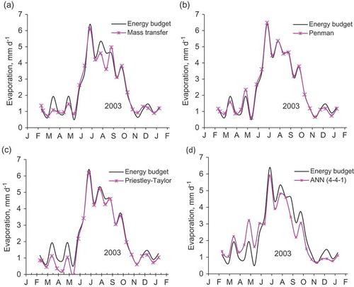
Figure 2. Daily evaporation rates, averaged per 15 days, estimated with the energy budget method for Lake Vegoritis during 2004, and compared to the (a) mass transfer, (b) Penman, (c) Priestley-Taylor, and (d) ANN methods.

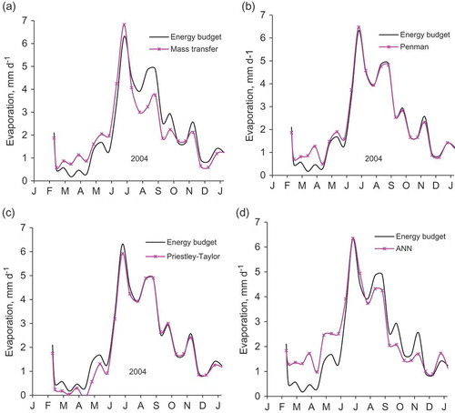
Evaporation rates estimated with the Penman method exhibit the closest agreement with the energy budget estimations, followed by the Priestley-Taylor and mass transfer methods. The mean rate of evaporation with the energy budget method is 2.53 mm d⁻¹ for the year 2003 and 2.48 mm d ⁻¹ for the year 2004. The mean evaporation rates calculated for the two years (2003 and 2004) of application are 2.26 and 2.08 mm d⁻¹ for the mass transfer method, 2.36 and 2.25 mm d⁻¹ for the Penman method, and 2.07 and 1.99 mm d⁻¹ for the Priestley-Taylor method, respectively. Regarding the energy budget method, it should be noted that if the values for the days excluded from the calculations were taken into account, then the mean annual evaporation rates would be smaller. If the evaporation rates for these days were filled with the respective values for the Penman method, the mean annual evaporation rates for the energy budget method would be 2.38 and 2.24 mm d⁻¹ for the years 2003 and 2004, respectively.

In Table 1, the results of statistical tests for the examined evaporation determination methods and data for the two years are correlated with the energy budget method. Specifically, the maximum and minimum monthly values and the average of the daily values of mean absolute error (MAE), root mean square error (RMSE), and coefficient of residual mass (CRM) are presented. The optimum values of MAE, RMSE and CRM are zero. The statistical tests confirm that the Penman method correlates better with the energy budget estimations, with MAE of 0.1–0.58 mm d⁻¹, while the RMSE was 0.12–1.02 mm d⁻¹. The CRM shows overestimation for February, June, July, September and October and underestimation for the other months. For the mass transfer method the MAE was 0.33–1.29 mm d⁻¹, the RMSE 0.43–1.53 mm d⁻¹ and CRM values show overestimation for two months, February and June. The evaporation rates evaluated with the Priestley-Taylor method in comparison with those estimated with the energy budget method give a MAE of 0.05–0.98 mm d ⁻¹ and RMSE of 0.09–1.61 mm d⁻¹. According to CRM, this method underestimates evaporation for all months except September.

Table 1. Statistical tests of the data from the evaporation estimation methods for the two years (MT: mass transfer; P: Penman; P-T: Priestley-Taylor; ANN: artificial neural network).

Monthly and yearly	MAE				RMSE				CRM
	MT	P	P-T	ANN	MT	P	P-T	ANN	MT	P	P-T	ANN
Max	1.29	0.58	0.98	1.77	1.53	1.02	1.61	2.55	0.30	0.10	0.62	0.21
Min	0.33	0.10	0.05	0.48	0.43	0.12	0.09	0.61	−0.19	−0.09	−0.01	−0.60
Average	0.73	0.21	0.28	1.20	1.01	0.39	0.59	1.79	0.07	0.00	0.09	0.00

Generally, the correlation of the energy budget evaporation rates with those of the Penman method is particularly good and with those of the mass transfer and Priestley-Taylor methods is very good. For the Penman and Priestley-Taylor methods the greater discrepancies occur in spring months when evaporation is low. These discrepancies are much larger for the Priestley-Taylor method. A possible explanation is that at this time of the year the sensible heat flux (H) often has negative values, which is a major constraint on using the Priestley-Taylor equation (Priestley and Taylor 1972, Dos Reis and Dias 1998). During summer and early autumn, the seasons of highest evaporation rates, agreement between the two methods and the energy budget method is extremely close. For the mass transfer method this is not the case, as significant discrepancies occur throughout the year. This is perhaps an indication that the energy term is very important in evaporation estimations, and equations that include it should be preferred. However, if there is difficulty in calculation of the energy components, the mass transfer method could be used with sufficient accuracy.

Rosenberry et al. (2007) indicated that Priestley-Taylor method provided the best values and the Penman method the next best values for evapotranspiration estimation related to the energy budget method, and the mass transfer method provided the worst correlations. Yao (2009) evaluated seven climate-based methods of evaporation estimation and concluded that the ranking of methods depended on the time step used for the estimations. The Penman and Priestley-Taylor are among the methods that work better than others regardless of the time step. Benzaghta et al. (2012) showed that, among the climate-based models, the Priestley-Taylor model gave a more accurate output when it was applied to predict evaporation from reservoirs in tropical climates.

4.2 Artificial neural networks method

The datasets of daily values of air temperature (T_a), relative humidity (RH), wind speed (u₂) and sunshine hours (n) were used as the input and the evaporation values estimated with the energy budget method (E_EB) were used as the output target variable in the derivation of the ANN technique. The four variables (T_a, RH, n, u₂) were standardized using Equation (14) before training and testing, and were used as input variables. The target output variable E_EB was also standardized before training and testing.

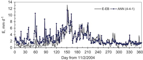
For the year 2003, 331 datasets of estimated evaporation (E_EB) values obtained using the energy budget method were used in the procedure to detect the most suitable ANN model architecture. From the total available datasets, 244 (73%) were used for training of the ANN model and the remaining 87 (27%) were employed for testing the model. In choosing the datasets for testing, special attention was paid to having representative sets for each class of evaporation values. For this reason, they were selected randomly from every 4–5 successive available daily values. For the number of neurons in the hidden layer, a trial and error procedure was used. The most appropriate model is of structure 4-4-1, which means that the model consists of 4 input variables, 4 neurons in the hidden layer and 1 in the output layer.

Figure 3a shows a comparison of evaporation values predicted by the ANN model of structure 4-4-1 versus the energy budget estimated values for the testing datasets. Figure 4 shows a comparison of evaporation values estimated using the ANN model and the energy budget method when 244 datasets were used for training and the total number of available datasets were used for evaluation. The RMSE and r values of the testing dataset were 1.09 mm d⁻¹ and 0.91, respectively. In the second case, RMSE and r for all the datasets were 0.84 mm d⁻¹ and 0.92, respectively.

Figure 3. Comparison of evaporation values predicted by the ANN method versus the energy budget method for the testing datasets for the years (a) 2003 and (b) 2004.

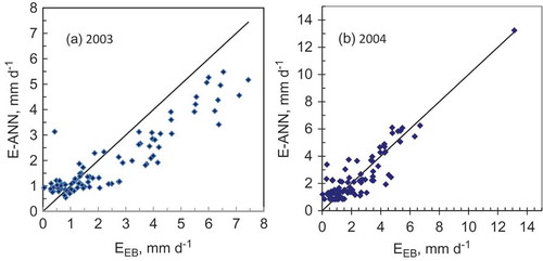
Figure 4. Comparison of evaporation values predicted by the ANN method versus the energy budget method for the total available datasets for the year 2003.

For the year 2004, 317 datasets of evaporation values (E_EB) estimated by the energy budget method were used to determine the most appropriate ANN model. From the total available datasets, 227 (72%) were used for training and the remaining 90 (28%) were used for testing the model. The selection of datasets for testing was based on random choices of one from every 4–5 successive available daily values. For the number of neurons in the hidden layer, the model architecture 4-4-1 was also used.

Figure 3(b) shows a comparison of evaporation values predicted by the ANN model of structure 4-4-1 versus the energy budget estimated values for the testing datasets for the year 2004, while Figure 5 shows a comparison of evaporation values estimated using the ANN model and energy budget method when 227 datasets for the year 2004 were used for training and all the available datasets were used for evaluation. The RMSE and r values of the testing dataset were 0.69 mm d⁻¹ and 0.89, respectively. In the second case RMSE and r for all the datasets were 0.75 mm d⁻¹ and 0.87, respectively.

Figure 5. Comparison of evaporation values predicted by the ANN method versus the energy budget method for the total available datasets for the year 2004.

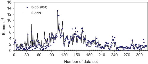
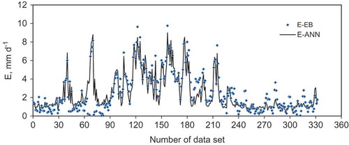
ANNs have been applied in recovery of missing data in hydrology, meteorology and water quality parameters. Diamantopoulou et al. (2007), as an example, applied the cascade correlation ANN models to estimate missing monthly values of water quality parameters in rivers. Using a derived ANN model for each year, the missing values of evaporation were estimated. Figure 6 presents the daily evaporation values estimated using the ANN model for 2003 (including 332 available and 33 missing data values for the year) in comparison with the energy budget method estimations. The statistical parameters of RSME and r between the evaporation values of the energy budget method and the ANN (4-4-1) model are 1.06 mm d⁻¹ and 0.86, respectively. The mean yearly evaporation rates with these methods are 2.36 and 2.47 mm d⁻¹, respectively.

Figure 6. Daily evaporation rates for Lake Vegoritis during 2003, with the missing values estimated and completed with the ANN model in comparison to values from the energy budget method.

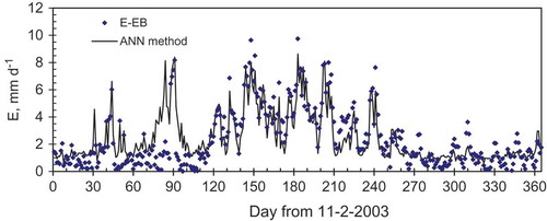
In another application, the time series of daily evaporation rates, completed with the missing data, for the years 2003 and 2004, were used to check the proposed ANN model. For this application the datasets of 365 daily evaporation rates for 2003 were used for training and the corresponding daily evaporation rates for 2004 were used to test/predict the ANN (4-4-1) model. Figure 7 presents the daily evaporation values estimated using the ANN model for 2004 (including the available and missing data for the year) in comparison with the energy budget method estimations. The statistical parameters of RSME and r between evaporation values of the energy budget method and the ANN (4-4-1) model are 1.35 mm d⁻¹ and 0.79, respectively. The mean yearly evaporation rate for the energy budget method is 2.25 mm d⁻¹, while for ANN it is 2.80 mm d⁻¹.

Figure 7. Daily evaporation rates for Lake Vegoritis during 2004, with the missing values estimated and completed with the ANN model in comparison to values from the energy budget method.

The statistical tests (MAE, RSME, CRM) of the ANN (4-4-1) model of Table 1 and the comparison of fortnightly values in relation to the energy budget method in Figures 1(d) and 2(d), show that the yearly average for MAE is 1.2 mm d⁻¹, with a range of monthly values from 0.5 to 1.77 mm d⁻¹, average RMSE is 1.79 mm d⁻¹ with a range from 0.61 to 2.55 mm d⁻¹ and CRM shows overestimation for January, March and April and underestimation for August to December. In comparison with the other methods examined the statistical tests are better, which may be due to the low flexibility of the ANN technique in describing the extreme values of inputs and outputs.

Accurate results of ANN techniques applied to predicting evaporation from lakes have been presented by other researchers, although the reference evaporation values originated from pan evaporation measurements. Goel (2009), in a study of pan evaporation under the conditions of a reservoir at Shegain, India, using ANN, also concluded that a combination of all input parameters provides better performance than using individual parameters in a model for estimating evaporation. Benzaghta et al. (2012) also indicated that an ANN with all input parameters provided better performance, with RMSE of 1.22 mm d⁻¹. Sammen (2013) concluded that a combination of all parameters provided better performance than individual parameters for the ANN (4-10-1) model in his study of the Hemren reservoir in Iraq.

5 Conclusions

Daily evaporation rates were estimated as a residual of the energy budget for Lake Vegoritis in northern Greece and for the climatic conditions of the years 2003 and 2004. Estimations using the energy budget method, considered the standard method, were compared with evaporation rates calculated with three other climate-based methods: the Penman, Priestley-Taylor and mass transfer methods. The Penman method correlated best with the energy budget method. The Priestley-Taylor and mass transfer methods showed very good correlation. The mean rates of evaporation with the energy budget method for the two years (2003 and 2004) of application were 2.53 and 2.48 mm d⁻¹, with the mass transfer method 2.26 and 2.08 mm d⁻¹, with the Penman method 2.36 and 2.25 mm d⁻¹ and with the Priestley-Taylor method 2.07 and 1.99 mm d⁻¹, respectively. The discrepancies between the Priestley-Taylor and the energy budget methods during the spring season were moderated when energy budget evaporation values of spring days excluded from the calculations were set to zero. Furthermore, in spring the sensible heat flux (H) often has negative values, which is a major constraint on using the Priestley-Taylor equation, thus resulting in these descrepancies.

Daily evaporation rates were also calculated using an ANN technique. Meteorological daily data for each year were used for model training and testing. The daily datasets for the two years were used to detect the most suitable structure for the ANN model using different magnitude datasets, either separately for each year or using one year for training and the other year for testing/prediction. The estimated values during the test procedure approach the dataset with RSME and correlation coefficient of 1.09 mm d⁻¹ and 0.91 for the year 2003 and 0.69 mm d⁻¹ and 0.89 for the year 2004, respectively. The mean rates of evaporation for the two years (2003 and 2004) of application were 2.27 and 2.36 mm d⁻¹, respectively.

The results for the training and the test datasets clearly demonstrated the ability of ANN models to predict very well the daily values of evaporation in lakes by using daily meteorological parameters, which are introduced as inputs to the chosen ANN models. The ANN models introduced in this study have the ability to develop a generalized solution and seem promising for application in the prediction of daily values of evaporation and allow the filling of missing values in their time series.

The availability of climatic data is a primary consideration in selecting an evaporation estimation method. The energy budget, Penman and Priestley-Taylor methods are data intensive, as they require measurement of many meteorological variables. The mass transfer method is less data demanding, requiring only surface water temperature, relative humidity and wind velocity. In the absence of adequate meteorological data, the mass transfer method can be used with sufficient accuracy.

Disclosure statement

No potential conflict of interest was reported by the authors.

References

- Antonopoulos, V.Z., Diamantidis, G., and Tsiouris, S., 1996. Vegoritis Lake: a review in hydrological and quality parameter changes. Geotechnical Scientific Bulletin, 7 (1), 63–78 (in Greek).
- Antonopoulos, V.Z., Georgiou, P.E., and Antonopoulos, Z.V., 2015. Dispersion coefficient prediction using empirical models and ANNs. Environmental Processes, 2, 379–394. doi:10.1007/s40710-015-0074-6
- Antonopoulos, V.Z. and Gianniou, S.K., 2003. Simulation of water temperature and dissolved oxygen distribution in Lake Vegoritis, Greece. Ecological Modelling, 160, 39–53. doi:10.1016/S0304-3800(02)00286-7
- Ariapour, A. and Zavarech, M.N., 2011. Estimation of daily evaporation using of artificial neural networks (Case study: Borujerd meteorological station). Journal of Rangeland Science, 2, 125–132.
- ASCE, 2000, Task Committee on Application of Artificial Neural Networks in Hydrology (2000). Artificial neural networks in hydrology II: hydrological applications. Journal of Hydrologic Engineering, 5 (2), 115–123. doi:10.1061/(ASCE)1084-0699(2000)5:2(115)
- Assouline, S. and Mahrer, Y., 1993. Evaporation from Lake Kinneret: 1. Eddy correlation system measurements and energy budget estimates. Water Resources Research, 29 (4), 901–910. doi:10.1029/92WR02432
- Benzaghta, M.A., et al., 2012. Prediction of evaporation in tropical climate using artificial neural network and climate based models. Scientific Research and Essays, 7 (36), 3133–3148.
- Bowie, G.L., Mills, W.B., and Porcella, D.B., 1985. Rates, constants and kinetics formulations in surface water quality modeling. EPA/600/3-85/040, Athens, USA.
- Cheung, C.-C., Ng, S.-C., and Lui, A.K., 2012. Improving the Quickprop algorithm. WCCI2012 IEEE World Congess on Computational Intelligence, Brisbane, Australia, 6 p.
- Diamantopoulou, M.J., Antonopoulos, V.Z., and Papamichail, D.M., 2007. Cascade correlation artificial neural networks for estimating missing monthly values of water quality parameters in rivers. Water Resources Management, 21, 649–662. doi:10.1007/s11269-006-9036-0
- Diamantopoulou, M.J., Georgiou, P.E., and Papamichail, D.M., 2011. Performance evaluation of artificialneyral networks in estimation references evapotranspiration with minimal meteorological data. Global Nest Journal, 13, 18–27.
- dos Reis, R. and Dias, N., 1998. Multi-season lake evaporation: energy-budget estimates and CRLE model assessment with limited meteorological observations. Journal of Hydrology, 208, 135–147. doi:10.1016/S0022-1694(98)00160-7
- Duan, Z. and Bastiaanssen, W.G.M., 2015. A new empirical procedure for estimating intra-annual heat storage changes in lakes and reservoirs: review and analysis of 22 lakes. Remote Sensing of Environment, 156, 143–156. doi:10.1016/j.rse.2014.09.009
- Fahlman, S.E., 1988. An empirical study of learning speed in back-propagation networks technical report CMU-CS-88-162. Carnegie-Mellon University.
- Gianniou, S.E. and Antonopoulos, V.Z., 2007b. Estimation of evaporation in Lake Vegoritis, Greece. In: G.P. Karatzas, et al., eds. Proceedings of EWRA symposium water resources management: new approaches and technologies, 14–16 June, Chania.
- Gianniou, S.E. and Antonopoulos, V.Z., 2014. Primary production and phosphorus modelling in Lake Vegoritis, Greece. Advances in Oceanography and Limnology, 5 (1), 18–40. doi:10.1080/19475721.2013.871579
- Gianniou, S.K. and Antonopoulos, V.Z., 2007a. Evaporation and energy budget in Lake Vegoritis, Greece. Journal of Hydrology, 345, 212–223. doi:10.1016/j.jhydrol.2007.08.007
- Goel, A., 2009. ANN based modeling for prediction of evaporation in reservoirs. International Journal of Engineering Transcations A: Basics, 22, 352–359.
- Goyal, M.K., et al., 2014. Modeling of daily pan evaporation in sub tropical climates using ANN, LS-SVR, fuzzy logic, and ANFIS. Expert Systems with Applications, 41, 5267–5276. doi:10.1016/j.eswa.2014.02.047
- Henderson-Sellers, B., 1984. Engineering Limnology. Great Britain: Pitman Publishing.
- Kalifa, E.A., Abd El-HadyRady, R.M., and Alhayawei, S.A., 2012. Estimation of evaporation losses from Lake Nasser: neural network based modeling versus multivariate linear regression. Journal of Applied Sciences Research, 8 (5), 2785–2799.
- Lenters, J., Kratz, T., and Bowser, C., 2005. Effects of climate variability on lake evaporation: results from a long-term energy budget study of Sparkling Lake, northern Wisconsin (USA). Journal of Hydrology, 308, 168–195. doi:10.1016/j.jhydrol.2004.10.028
- Mantoglou, A., 2003. Estimation of heterogeneous aquifer parameters from piezometric data using ridge functions and neural networks. Stochastic Environmental Research and Risk Assessment (SERRA), 17, 339–352. doi:10.1007/s00477-003-0155-3
- Momii, K. and Ito, I., 2008. Heat budget estimates for Lake Ikeda, Japan. Journal of Hydrology, 361, 362–370. doi:10.1016/j.jhydrol.2008.08.004
- Papamichail, D. and Antonopoulos, V.Z., 1998. Analysis of Vegoritis lake water balance deficit. In: K.L. Katsifarakis, et al., eds. Proc. int. conf. protection and restoration of the environment IV, 1–4 July, Halkidiki, Greece.
- Payero, J., et al., 2003. Guidelines for validating Bowen ratio data. Transactions of the ASAE, 46 (4), 1051–1060. doi:10.13031/2013.13967
- Penman, H., 1948. Natural evaporation from open water, bare soil and grass. Proceedings of the royal society A: mathematical, physical and engineering sciences, 193, 120–145. doi:10.1098/rspa.1948.0037
- Piotrowski, A.P., Rowinski, P.M., and Napiorkowski, J.J., 2012. Comparison of evolutionary computation techniques for noise injected neural network training to estimate longitudinal dispersion coefficients in rivers. Expert Systems with Applications, 39, 1354–1361. doi:10.1016/j.eswa.2011.08.016
- Priestley, C. and Taylor, R., 1972. On the assessment of surface heat flux and evaporation using large-scale parameters. Monthly Weather Review, 100 (2), 81–92. doi:10.1175/1520-0493(1972)100<0081:OTAOSH>2.3.CO;2
- Rosenberry, D.O., et al., 2007. Comparison of 15 evaporation methods applied to a small mountain lake in the Northeastern U.S.A. Journal of Hydrology, 340, 149–166. doi:10.1016/j.jhydrol.2007.03.018
- Sacks, L., Lee, T., and Radell, M., 1994. Comparison of energy budget evaporation losses from two morphometrically different Florida seepage lakes. Journal of Hydrology, 156, 311–334. doi:10.1016/0022-1694(94)90083-3
- Sammen, S.S., 2013. Forecasting of evaporation from Hemren reservoir by using artificial neural network. Diyala Journal of Engineering Sciences, 6 (4), 38–33.
- Sene, K., Gash, J., and McNeil, D., 1991. Evaporation from a tropical lake: comparison of theory with direct measurements. Journal of Hydrology, 127, 193–217. doi:10.1016/0022-1694(91)90115-X
- Singh, V. and Xu, C., 1997. Evaluation and generalization of 13 mass-transfer equations for determining free water evaporation. Hydrological Processes, 11, 311–323. doi:10.1002/(ISSN)1099-1085
- Sturrock, A., Winter, T., and Rosenberry, D., 1992. Energy budget evaporation from Williams Lake: a closed lake in north central Minnesota. Water Resources Research, 28 (6), 1605–1617. doi:10.1029/92WR00553
- Tanner, B., Greene, J., and Bingham, G., 1987. A Bowen ratio design for long term measurements, Proc. ASAE, 1987 International Winter Meeting, St. Joseph, MI.
- Tayfur, G. and Singh, V.P., 2005. Predicting longitudinal dispersion coefficient in natural streams by artificial neural network. Journal of Hydraulic Engineering, ASCE, 131 (11), 991–1000. doi:10.1061/(ASCE)0733-9429(2005)131:11(991)
- Terzi, O. and Keskin, M.E., 2010. Comparison of artificial neural networks and empirical equations to estimate daily pan evaporation. Irrigation and Drainage, 59, 215–225.
- Valiantzas, J., 2006. Simplified versions for the Penman evaporation equation using routine weather data. Journal of Hydrology, 331, 690–702. doi:10.1016/j.jhydrol.2006.06.012
- Winter, T., et al., 2003. Evaporation determined by the energy-budget method for Mirror Lake, New Hampshire. Limnology and Oceanography, 48 (3), 995–1009. doi:10.4319/lo.2003.48.3.0995
- Wu, W., Dandy, G.C., and Maier, H.R., 2014. Protocol for developing ANN models and its application to the assessment of the quality of the ANN model development process in drinking water quality modelling. Environmental Modelling & Software, 54, 108–127. doi:10.1016/j.envsoft.2013.12.016
- Yao, H., 2009. Long-term study of lake evaporation and evaluation of seven estimation methods: results from Dickie Lake, south-central Ontario, Canada. Journal of Water Resource and Protection, 2, 59–77. doi:10.4236/jwarp.2009.12010