Groundwater system response at sites with different agricultural land uses: case of the Guarani Aquifer outcrop area, Brotas/SP-Brazil

ABSTRACT

A system identification approach can be incorporated in groundwater time series analysis, revealing information concerning the local hydrogeological situation. The aim of this work was to analyse water table fluctuations in an outcrop area of the Guarani Aquifer System (GAS) in Brotas/SP, Brazil, using data from a groundwater monitoring network. The water table dynamic was modelled using continuous time series models that reference the hydrogeological system upon which they operate. The model’s climatological inputs of precipitation and evapotranspiration generate impulse response (IR) functions with parameters that can be related to the physical conditions concerning the hydrological processes involved. The interpretation of the model parameters from two sets of monitoring wells selected at different land-use sites is presented, exemplifying the effect of different water table depths and the distance to the nearest drainage location. Systematic trends of water table depths were also identified from model parameters at specific periods and related to plant development, crop harvest and land-use changes.

EDITOR D. Koutsoyiannis

ASSOCIATE EDITOR L. Ruiz

KEYWORDS:

• Time series analysis
• statistical modelling
• land use
• Brazil

1 Introduction

Land use and agricultural activities developed in geographical space place pressure on water resources. The interactions of soil, water, plants and the atmosphere cause fluctuations in groundwater levels. Agricultural systems planning and implementation depend on the availability of natural resources. The availability of groundwater, surface water and water from precipitation in a region determines not only crop choices but also management practices. Time series models provide an elegant solution to modelling scarce and irregularly sampled monitoring data on water table depths in a continuous way. Generally, the derivation of time series model parameters is primarily a statistical exercise based on the properties of the data. However, time series analysis can be extended through a system identification approach, revealing information about system properties (e.g. in the case of groundwater, local hydrogeological conditions are revealed). System identification was a term coined by Zadeh (1956) to deal with the problem of building mathematical models of dynamic systems based on observed data. In general, system identification methods are applied when a purely physical model would be excessively complex or impossible to obtain in a reasonable time, due to the complex nature of many systems and processes. Von Asmuth (2012) stated that in a system identification or time series analysis scope, it is common practice to denote forcing variables as input and forced variables as output. The behaviour of a system is the way in which the system responds or behaves when it is stimulated. If a calibrated time series model for a monitoring well presents physically-based parameters and can be extended for a set of monitoring wells in a catchment or a region, then relevant information about previous, actual and future states of a hydrological system can be derived from this model and incorporated in a soil and/or water management programme.

The aim of this work is to analyse the time series data from a groundwater monitoring network collected semi-monthly for a period of 10 years in an outcrop area of the Guarani Aquifer System (GAS) in Brotas, São Paulo, Brazil. A system identification approach was used to test whether differences in water table behaviour are due to various factors including land use, management, crop water interception and consumption. These factors are considered the major differences and influences on aquifer dynamics imposed by agricultural land use in the region.

2 Materials and methods

2.1 Study area

The study area is located between 22°10′–22°15′S and 47°55′–48°00′W in the municipality of Brotas, province of São Paulo, Brazil, in a land development called Lagoa Dourada, near the Onça Creek watershed, an effluent of the Jacaré-Guaçú River (Fig. 1). This area presents a small settlement of weekend houses and farms with land uses typical for São Paulo province, such as sugarcane, reforestation (with Eucalyptus), citrus, pasture and some spots of natural Cerrado vegetation.

Figure 1. Map of Brazilian territory and its provinces with detail of the Onça Creek watershed.

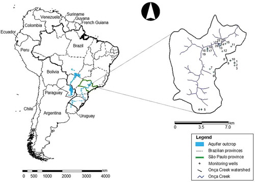
The area and surroundings are an outcrop zone of the Guarani Aquifer System (GAS), composed of sandy rocks of Triassic age from the Piramboia Formation and Aeolian sandstones from the Botucatu Formation, which are Jurassic–Neo-Cretaceous in age. This sequence is bounded at the base and top by two regional unconformities, which separate the GAS from the Palaeozoic and Neo-Cretaceous units (Gastmans et al. 2010, 2012). The major water body in the area, the Onça Creek, flows mainly over the Botucatu Formation and, at the basin outlet, over the Botucatu-basalt complex. Both units belong to the São Bento group of Mesozoic age. Cenozoic soils present in the area are the result of sandstone weathering; the soil exhibits a homogeneous sand composition with no loam (Wendland et al. 2007). The Botucatu Formation comprises well-sorted, very-fine- to fine-grained aeolian sandstones with cross-stratifications of medium to great thickness (Caetano-Chang 1997, Sracek and Hirata 2002).

2.2 Monitoring data

In the Lagoa Dourada area, the LHC/SHS/EESC/USP (Computational Hydraulics Lab/Department of Hydraulics and Sanitary Engineering/São Carlos School of Engineering/University of São Paulo) team has monitored groundwater levels at 23 wells in the GAS outcrops since 2004. Water table depths were manually observed every 15 days from April 2004 to June 2014, totalling 10 years of observations. The locations of these wells were selected to cover the range of land uses and hydrogeological domains in the area, in an attempt to characterize the different responses of water table depths in the basin. The screening filter levels of the wells varied with soil depth, from a few metres close to drainages to a maximum of 161 m in the southern part of the watershed.

Time series of daily precipitation and potential evapotranspiration were available from the Centre for Water Resources and Applied Ecology of the University of Sao Paulo (CRHEA/USP), who have collected climatological data continuously near the Broa Reservoir, 1.5 km away from the Lagoa Dourada wells. Daily weather data were also available from four automatic weather stations located in different land-use sites (pasture, sugarcane, citrus and natural Cerrado vegetation). Actual and potential evapotranspiration were calculated using the FAO Penman-Monteith method, considering the crop coefficient (K_c) from each culture according to FAO (1998). Because we considered all selected wells to be in the same porous domain and of the same soil type, the only differences in the water table behaviour between the wells should be related to the thickness of the unsaturated zone, the distance to drainage and the vegetation influences.

2.3 Time series modelling

For water table depths, the dynamic relationship between precipitation and water table depth can also be described using physical mechanistic groundwater flow models. However, much less complex transfer function-noise model predictions of the water table depth can be obtained which are often as accurate as those obtained by physical mechanistic modelling (Knotters 2001). Transfer function-noise models (Box and Jenkins 1970, Hipel and McLeod 1994) have been successfully applied to describe the dynamic relationship between precipitation surplus and water table depths in several studies, due to their simplicity when compared with other modelling approaches, using less data and being less computer time consuming (Tankersley and Graham 1994, Knotters and Van Walsum 1997, Van Geer and Zuur 1997, Yi and Lee 2003, Von Asmuth and Knotters 2004, Manzione et al. 2010).

2.3.1 PIRFICT model

We used the Predefined Impulse Response Function In Continuous Time model (PIRFICT; Von Asmuth et al. 2002), which is based on a special type of transfer function-noise model in continuous time, as an alternative to the discrete time series models. It is implemented in the computer package Menyanthes (Von Asmuth et al. 2012).

In the PIRFICT model, a series of block pulses of the input is transformed into an output series by a continuous-time transfer function, the coefficients of which do not depend on the observation frequency. In the simple case of a linear, undisturbed phreatic system that is influenced by precipitation surplus only, the following multiple inputs create a continuous transfer function-noise model, written as a convolution integral, which can be used to model the relationship between water table dynamics and the precipitation surplus or deficit:

(1)

(2)

(3)

where h is the observed water table depth at time t [T]; h_i* is the predicted water table depth at time t attributed to stress i, relative to d [L]; d is the level of h*(t) without precipitation, i.e. the local drainage level relative to the ground surface [L]; r is the residuals series [L]; R_i is the value of stress i at time t [L/T]; θ is the transfer impulse response (IR) function [–]; ϕ is the noise impulse response (IR) function [–]; and W is a continuous white noise (Wiener) process with the properties E{dW(t)} = 0, E[{dW(t)}²] = βdt, E[dW(t₁)dW(t₂)] = 0 for t₁ ≠ t₂ [L] and β a parameter [L²/T].

Von Asmuth et al. (2008) stated that IR functions can be identified by the types of stress that affect the behaviour of water table depths, including precipitation, evapotranspiration, groundwater withdrawal (or injection), surface water levels, barometric pressure and hydrological interventions. From the many types of stress, R_i, in this study h_i*(t) is attributed to the precipitation and actual crop evapotranspiration stresses, and modelled as the transfer function noise or PIRFICT model. In other words, h_i*(t) of Equation 2 is defined as the sum of the effects of the precipitation and evapotranspiration series as follows:

(4)

(5)

where p is the precipitation intensity at time t [L/T]; et is the evapotranspiration intensity at time t [L/T]; and f [–] is a reduction function for et dependent on soil water shortages and land cover.

In general, groundwater systems react differently to the different stresses they are submitted to. However, there are also cases where different stresses cause similar responses, such as precipitation and evapotranspiration. The effect of evapotranspiration et on the water table depth h is the same as p, but negative, except for the reduction factor f. When Equations (4) and (5) are added together as in the first term of Equation (1), evapotranspiration is subtracted from precipitation, which is similar to a water balance.

The local drainage level d is estimated from the data as follows:

(6)

where N is the number of water table depth observations.

An important advantage in the use of the PIRFICT model here, compared with the discrete-time transfer function-noise models, is that it can address input and output series that have different observation frequencies or irregular time intervals (Von Asmuth and Bierkens 2005). After calibration, the physical plausibility of the results is verified by inspecting the IR functions obtained for each well (which are linked to the cross-correlation functions).

2.3.2 Model selection criteria

After the observed time series had been modified by linear interpolation and a resampling operation during model fitting, the explained variance percentage (EVP) was calculated to measure the variance of the groundwater series and the residual series (Von Asmuth 2012) for each individual well monitored in the Lagoa Dourada area. In the EVP calculation, the residual variance was weighted according to the variance of the original signal. Errors from the transfer model were evaluated using root mean squared errors (RMSE) and the variance of the noise processes using root mean squared innovations (RMSI), as discussed by Von Asmuth and Bierkens (2005). The adjustments of IR functions to data were verified during the simulation procedure of the PIRFICT model, checking the number of interactions and the best model order from the automatic fit using the Akaike information criterion (AIC) and final prediction error (FPE) values. These values indicate a relative estimate of the information lost when the model tries to represent the process that generates the data. The FPE criterion provides a measure of model quality by simulating the situation where the model is tested on a different dataset; this is done by computing several different models and then comparing them using this criterion, with the most accurate model having the smallest FPE. This is a logical way of comparing model results from automatic model order selection criteria, but as both AIC and FPE use the innovation variance for determining the best model order, they cannot be used to compare models with different variances or datasets (Von Asmuth 2012).

2.4 Groundwater system identification

Considering that differences in soil management, crop type, plant development and agricultural practices have a direct impact on the unsaturated zone and recharge rates, water tables will respond differently under different local conditions. The adjusted IR function can describe how the water table responds to a change in precipitation surplus or deficit. When used for modelling groundwater level monitoring series, the IR function parameters define the shape of the distribution function and have no direct physical meaning; however, in the case of the response to precipitation and evapotranspiration, the parameters have a wide range of variability that can be related to hydrogeological local conditions. A typical IR function looks similar to a highly skewed probability distribution function. For example, θ_p is typically treated as a scaled gamma distribution function (SG df, Von Asmuth 2012), which can model the response of a broad range of groundwater systems. Assuming linearity, the deterministic part of the water table dynamics may be characterized by the moments of the IR function. In such cases, based on Von Asmuth et al. (2008), the IR function and its parameters for precipitation surplus/deficit can be defined as:

(7)

(8)

where A, a and n are parameters that define the shape of the SG df; Γ(n) is the gamma function; α controls the decay rate of ϕ(t); and σ_r² is the variance of the residuals.

The form and area of the IR function depend strongly on the local hydrological conditions. The parameter A is the area of the SG df and is related to the local drainage resistance. The area of the IR function is also the ratio of the mean convexity of the groundwater head above the local drainage base to the mean groundwater recharge when, for instance, the flow resistance to the nearest drainages is small. The water table would drop quickly after a precipitation input and consequently the area of the IR function would be small. With increasing drainage resistance, the decay rate a of the responses decreases (a ≈ 1/A), i.e. the water table would drop slowly when the drainage resistance is high (Von Asmuth 2012). Parameter a is determined by the storage coefficient of the soil and n is the convection and dispersion time of the precipitation through the unsaturated zone. The physical basis of the SG df describes the transfer function of a series of linear reservoirs (Nash 1958). A single linear reservoir (SG df where n = 1) corresponds to a simple physical model of a one-dimensional soil column, the discharging lateral flow and functioning of the unsaturated zone. The storage coefficient, or porosity and soil moisture in the soil, determines the response of the system. Parameter n is the number of linear reservoirs and allows the SG df to take shapes gradually ranging from steeper than exponential to a Gaussian shape, combining two physical properties. Von Asmuth (2012) explained that, first, this behaviour resembles the effect of the relative position of a location within a system and, second, especially for n > 1, this behaviour resembles the effect of convection and dispersion of water in the unsaturated zone.

2.4.1 Monte Alegre and Santa Maria da Fábrica wells

In order to exemplify a system identification procedure from PIRFICT model calibrations, we selected two groups of four wells each to discuss differences in the IR functions due different local conditions. The land-use changes during the monitoring period were assessed using satellite images.

The first group of wells, numbered 16, 17, 18 and 19, are located on a hillside on the Monte Alegre farm. This toposequence, typical in the Onça Creek watershed, is a convex-shaped hill with a broad top that has a ramp of over 1500 m length and a height difference of approximately 68 m. The slope ranges from 3.2% in the upper third to 5.0% in the middle third and 9.0% in the lower third, with breaks in the slope perceived from the ground. The land use in this area was pasture for cattle from 2004 to 2011, while in January 2011, approximately 43 ha of the pasture area of the Monte Alegre farm, where wells 16–19 are located, was reforested with Eucalyptus for timber. The pasture was in an advanced stage of degradation, where the roots do not explore more than 0.50 m of soil, as verified in the field in 2010. In the early months of 2011, the land was ploughed, limed and fertilized, and then potted Eucalyptus were transplanted. The rainfall of the Brazilian summer enables Eucalyptus to grow quickly, developing taproots that can reach several metres in length in a few years.

The second group of four wells are located on the Santa Maria da Fábrica farm, in an area cultivated with citrus: two (W13 and W14) under citrus trees and two (W20 and W22) in the riparian vegetation close to Onça Creek. These wells exemplify the effect of distance to nearest drainage in the model parameters. Because wells 13 and 14 are located in an irrigated citrus field, we assume that the trees do not suffer water deficits for long periods because, in this zone, water for irrigation is readily available from the Onça Creek. In general, 90% of citrus roots are found in the top 40 cm of soil when cultivated in sandy soils under irrigation (Souza et al. 2007). In October 2013, the parcel of Santa Maria da Fábrica farm where wells 13 and 14 are located was renovated; the old citrus trees were removed and cultivation of sugarcane was initiated over an area of 13 ha.

3 Results

3.1 Modelling water table level monitoring data

The PIRFICT model fitted the observed time series well, with EVP being larger than 68% in all cases (Table 1). The lowest percentages in model adjustment might be caused by errors in the data or lack of data, or possibly other factors affecting the groundwater dynamics that are not incorporated into the model (Von Asmuth et al. 2002). Model errors were small, with RMSE values ranging from 0.05 to 1.16 m and RMSI from 0.04 to 0.41 m. Together with AIC and FPE (not shown), these results suggest that the model calibration can be considered as acceptable, considering the range of variation of water table levels and the fact that manual measurements themselves may contain errors, for example data transcription errors.

Table 1. Summary of model calibration statistics.

Well	EVP	RMSE	RMSI
W02	83.21	0.81	0.48
W03	78.79	0.25	0.18
W04	87.30	0.27	0.08
W05	82.48	0.32	0.14
W07	96.20	0.69	0.28
W08	71.67	1.16	0.51
W09	98.02	0.30	0.11
W10	98.46	0.18	0.07
W11	86.46	0.29	0.21
W12	75.57	0.81	0.42
W13	71.01	0.54	0.27
W14	74.35	0.50	0.24
W15	82.33	0.40	0.18
W16	84.65	0.30	0.13
W17	84.69	0.54	0.28
W18	81.40	0.83	0.39
W19	82.22	0.78	0.36
W20	78.25	0.22	0.12
W22	77.21	0.13	0.07
W23	86.24	0.06	0.05
W24	98.98	0.05	0.04
W25	84.43	0.58	0.32
W26	76.98	1.00	0.43
Mean	82.90	0.46	0.23
Min	68.72	0.05	0.04
Max	98.98	1.16	0.51

EVP: explained variance percentage (%), RMSE: root mean square error (m), RMSI: root mean square innovations (m).

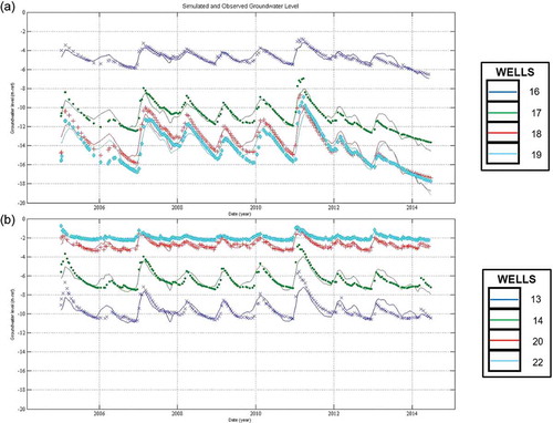
The temporal variations of water table level were captured well by the models, with some inconsistences in the beginning of the series and some peaks of water table fluctuation (Fig. 2). These occur because of the warming-up period of time series modelling and the smoothing effect, respectively (Hipel and McLeod 1994). The problem of peak estimation can be overcome by simulating multiple realizations of time series models (Manzione et al. 2010).

Figure 2. Calibrated time series model for wells (a) 16, 17, 18 and 19 and (b) 13, 14, 20 and 22 (solid lines) and water table level observations (symbols).

3.2 Physical interpretation of time series models

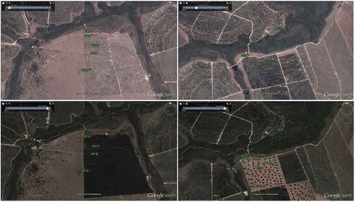
The groups of wells on the Monte Alegre and Santa Maria da Fábrica farms are approximately 2 km apart. Both areas had land-use changes during the monitoring period (Fig. 3).

Figure 3. Land-use evolution on the Monte Alegre (left) and Santa Maria da Fábrica (right) farms at 25 July 2011 (top) and 12 October 2013 (bottom).

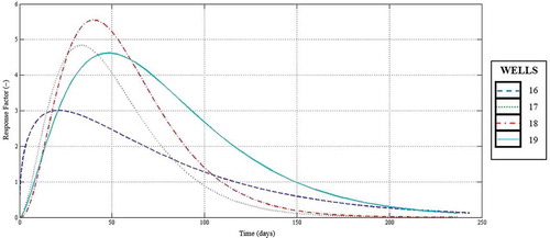
In the Monte Alegre wells, the influence of the unsaturated zone thickness on the water table behaviour was evident and all wells responded to the same precipitation and evapotranspiration time series inputs. Parameter A was higher in the deeper wells (Table 2), revealing a large drainage resistance and a long memory of the hydrogeological system. In other words, at wells 18 and 19, it takes more time for the effect of an input of precipitation to the groundwater levels to fade away, and the well would respond slowly to climate fluctuations. The smaller the storage coefficient a, the more the water table would rise as a result of a unit input of precipitation. However, the drainage resistance A is higher when the decay rate a is kept constant. The shape of the IR functions calibrated for the precipitation surplus into the groundwater system illustrates the memory of the system and the response after precipitation inputs expressed in days (Fig. 4).

Table 2. PIRFICT-model parameters and standard deviations (in parentheses) of parameters calibrated from the monitoring time series.

Well	A	a	n	f	e	LDB
W13	351.70 (51.00)	0.0336 (0.008)	2.04 (0.34)	1.05 (0.20)	99.74 (15.82)	−8.28
W14	301.30 (48.00)	0.0308 (0.008)	1.79 (0.31)	0.67 (0.24)	106.62 (16.27)	−5.24
W16	307.00 (42.00)	0.0186 (0.005)	1.39 (0.19)	0.82 (0.17)	123.96 (17.38)	−3.75
W17	307.10 (45.00)	0.0569 (0.018)	2.90 (0.70)	0.78 (0.22)	99.38 (17.21)	−8.81
W18	374.20 (71.00)	0.0595 (0.025)	3.38 (1.10)	0.83 (0.28)	106.53 (16.93)	−10.50
W19	466.80 (83.00)	0.0329 (0.011)	2.59 (0.63)	0.51 (0.30)	111.65 (16.92)	−9.96
W20	183.50 (22.00)	0.0246 (0.006)	1.19 (0.13)	1.09 (0.15)	64.89 (11.86)	−2.40
W22	60.52 (8.90)	0.0483 (0.021)	1.06 (0.22)	0.57 (0.23)	27.21 (3.01)	−1.61

A: drainage resistance (d), a: storage coefficient (1/d), n: number of linear reservoir (–), f: evapotranspiration factor, e: noise parameter (–), LDB: average local drainage base (m).

Figure 4. IR functions for precipitation at wells 16, 17, 18 and 19.

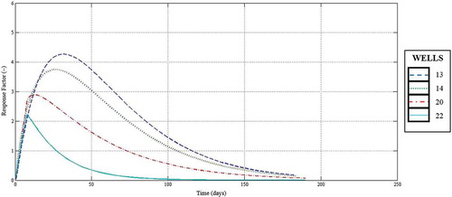
In the Santa Maria da Fábrica monitoring wells, wells 20 and 22 are closer to Onça Creek than wells 13 and 14. Consequently, parameter A was smaller at the latter sites, denoting a faster response due to precipitation inputs. These differences can be captured by examining the estimated IR functions of each well (Fig. 5). The IR function peak for wells 20 and 22 was fast because of the soil moisture content and the rapid percolation close to the creek. The peak was also fast for the pasture because the degraded vegetation is unable to make full use of the soil water in the absence of efficient root uptake. Comparing the two groups of wells, the area of the IR functions for pasture was larger than that for citrus.

Figure 5. IR functions for precipitation at wells 13, 14, 20 and 22.

4 Discussion

The interpretation of the parameters of the SG df, or any other time series model, should be a careful procedure because of their lumped and empirical nature (Von Asmuth and Knotters 2004). Assessing the physical plausibility of the results of a TFN model begins with checking the IR functions, which are linked to the cross-correlation functions of the time series. The memory of the hydrological system can be indicated by the time lag for the IR function to approach zero, which should be covered by the monitoring period (De Gruijter et al. 2006). Additionally, the stochastic part of the model allows one to account for model errors and uncertainty. When comparing wells from different land uses with similar local drainage bases (LDB), such as W13 and W17, parameter A is higher for W13 even with W17 presenting deeper levels, but checking the standard deviation (SD) of the parameters, the wells are highly similar. Von Asmuth (2012) highlighted that for n ≠ 1 the y-intercept of the SG df is either zero or ∞, in which case the storage coefficient cannot be determined exactly. This is what happens in this case, where all n parameters are higher than 1, e.g. for well 18, n > 3. As Von Asmuth (2012) explains, with an increasing value of n, the influence of the unsaturated zone increases and the pulses of precipitation and evapotranspiration are increasingly dispersed and delayed. The SD of these parameters is low, also indicating good model performance. Evapotranspiration IR functions can be checked by the f parameter. Here, the evapotranspiration IR function worked as a water budget, discounting the influence of evapotranspiration into precipitation. Parameter e denotes the decay rate of the exponential function adjusted to each well. In general, the decays follow the memory of the system, being larger in the presence of long memories and smaller in cases of fast response.

From summer 2011/12 to June 2014, the wells at Monte Alegre farm (W16–W19) presented a systematic and large decline of the water table levels (Fig. 4). This can be explained by the large amount of evapotranspiration by Eucalyptus, whose root systems often extend more than 1 m below ground level and can be more than 10 m deep where physical conditions permit root penetration (Le Maitre et al. 1999). Hence, eucalyptus plantations drastically reduce the groundwater to recharge, resulting in deeper water levels. The dry summer of 2013/14 also contributed to these trends. The influence of plant type should be investigated further by long-term monitoring of water levels.

We have illustrated the potential of the PIRFICT model for identifying aquifer system characteristics using only 8 of the 23 wells available in our study. Once information about the groundwater system is identified, it can support the groundwater system conceptualization and provide calibration targets for a steady groundwater model (Obergfell et al. 2013). Among the remaining wells, some did not show good model calibration performance, i.e. the IR function did not capture the physical relationship between input and output series. The basis of the PIRFICT model lies in two fundamental and simple principles, mass conservation and Darcy’s law, represented by the continuity and constitutive equations, respectively (Von Asmuth 2012). When the model does not explain an observation satisfactorily, it suggests that possible other perturbations not included in the model are controlling the water table behaviour. For those situations, more input variables can be introduced in the model, such as pumping rates, river discharge and step trends (Von Asmuth et al. 2008), or detailed hydrogeological studies are required. Depending on available data and objectives of the study, information from the IR functions might not be required, and a good statistical adjustment can be sufficient to estimate past values and predict future values of the time series (Manzione et al. 2010).

This study revealed different responses of the water table and their relationship with local soil and crop influences. We propose that the information identified from the plausibility checking of the PIRFICT model parameters and its IR functions can be valuable for decision making, groundwater management and scenario evaluations. Aquifer outcrops are strategic areas for recharge and present natural vulnerability to groundwater contamination. Water level simulation based on past climatological conditions allows estimation of the actual status of the aquifer and prediction of future states. Information about the memory of the groundwater system interpreted as the time that an input takes to cause a response in the water table can help in selecting species for a land-use change, planning exploitation of wells, application of pesticides based on the half-life of the molecules in the unsaturated zone, water table control, dewatering and drainage infrastructures design. Insights into the main hydrological processes at stake in our study area can guide studies in other outcrop areas of the GAS. Understanding aquifer dynamics in those areas and incorporating this information into water resources management plans are key elements for success in the decision-making process.

5 Conclusions

The PIRFICT model was able to simulate water levels, identify groundwater system properties and estimate trends in water level in the Guarani Aquifer System outcrop area. It captured the variations of the water table well, and highlighted their relationship with seasonal patterns of rainfall. It revealed different responses of the water table and connections with local soil and crop conditions.

The area and amplitude of the presented IR functions varied with the type of vegetation, depth of water levels and distance to nearest drainage, denoting large memories of the groundwater system in areas far from drainage, with the deepest levels and no demanding vegetation, such as degraded pasture.

The influence of eucalyptus reforestation since 2011 in areas previously occupied by pasture and cattle deserves attention because of the negative linear trends estimated since then.

Disclosure statement

No potential conflict of interest was reported by the authors.

Additional information

Funding

This work was supported by FAPESP (São Paulo Research Foundation) and CNPQ (Brazilian National Council for Scientific and Technological Development) - [2011/11484-3].

References

- Box, G.E.P. and Jenkins, G.M., 1970. Time series analysis: forecasting and control. San Francisco: Holden-Day.
- Caetano-Chang, M.R., 1997. A Formação Pirambóia no centro-leste do estado de São Paulo. Thesis (PhD). Instituto de Geociências e Ciências Exatas – Rio Claro, Universidade Estadual Paulista (UNESP), Rio Claro. (In Portuguese)
- De Gruijter, J.J., et al., 2006. Sampling for natural resources monitoring. Berlin: Springer.
- FAO (Food and Agriculture Organization of the United Nations), 1998. Crop evapotranspiration - guidelines for computing crop water requirements - FAO Irrigation and drainage paper 56. Rome: FAO.
- Gastmans, D., et al., 2012. Modelo hidrogeológico conceptual del Sistema Acuífero Guaraní (SAG): una herramienta para la gestión. Boletín Geológico y Minero, 123 (3), 249–265. (In Spanish).
- Gastmans, D., Chang, H.K., and Hutcheon, I., 2010, Groundwater geochemical evolution in the northern portion of the Guarani Aquifer System (Brazil) and its relationship to diagenetic features. Applied Geochemistry, 25 (1), 16–33. doi:10.1016/j.apgeochem.2009.09.024
- Hipel, K.W. and McLeod, A.I., 1994. Time series modeling of water resources and environmental systems. Amsterdam: Elsevier.
- Knotters, M., 2001. Regionalised time series models for water table depths. Thesis (PhD). Wageningen University.
- Knotters, M. and Van Walsum, P.E.V., 1997. Estimating fluctuation quantities from time series of water-table depths using models with a stochastic component. Journal of Hydrology, 197, 25–46. doi:10.1016/S0022-1694(96)03278-7
- Le Maitre, D.C., et al., 1999. A review of information on interactions between vegetation and groundwater. Water SA, 25, 137–152.
- Manzione, R.L., et al., 2010. Transfer function-noise modeling and spatial interpolation to evaluate the risk of extreme (shallow) water-table levels in the Brazilian Cerrados. Hydrogeology Journal, 18 (8), 1927–1937. doi:10.1007/s10040-010-0654-5
- Nash, J.E., 1958. Determining runoff from rainfall. Proceedings of the Institution of Civil Engineers, 10, 163–184. doi:10.1680/iicep.1958.2025
- Obergfell, C., et al., 2013. Deriving hydrogeological parameters through time series analysis of groundwater head fluctuations around well fields. Hydrogeology Journal. doi:10.1007/s10040-013-0973-4
- Sracek, O. and Hirata, R., 2002. Geochemical and stable isotopic evolution of the Guarani Aquifer System in the state of São Paulo, Brazil. Hydrogeology Journal, 10, 643–655. doi:10.1007/s10040-002-0222-8
- Souza, L.D., Souza, L. da S., Ledo, C.A. de S., 2007. Sistema radicular dos citros em Neossolo Quartzarênico dos Tabuleiros Costeiros sob irrigação e sequeiro. Pesquisa Agropecuária Brasileira, 42, 1373–1381. doi:10.1590/S0100-204X2007001000002. (In Portuguese.)
- Tankersley, C.D. and Graham, W.D., 1994. Development of an optimal control system for maintaining minimum groundwater levels. Water Resources Research, 30, 3171–3181. doi:10.1029/94WR01790
- Van Geer, F.C. and Zuur, A.F., 1997. An extension of Box-Jenkins transfer/noise models for spatial interpolation of groundwater head series. Journal of Hydrology, 192, 65–80. doi:10.1016/S0022-1694(96)03113-7
- Von Asmuth, J.R., et al., 2002. Transfer function noise modeling in continuous time using predefined impulse response functions. Water Resources Research, 38 (12), 23-1–23-12. doi:10.1029/2001WR001136
- Von Asmuth, J.R., et al., 2008. Modeling time series of ground water head fluctuation subjected to multiple stresses. Ground Water, 46, 30–40.
- Von Asmuth, J.R., 2012. Groundwater system identification through time series analysis. Thesis (PhD). TU Delft.
- Von Asmuth, J.R. and Bierkens, M.F.P., 2005. Modeling irregularly spaced residual series as a continuous stochastic process. Water Resources Research, 41, W12404. doi:10.1029/2004WR003726
- Von Asmuth, J.R. and Knotters, M., 2004. Characterising groundwater dynamics based on a system identification approach. Journal of Hydrology, 296, 118–134. doi:10.1016/j.jhydrol.2004.03.015
- Von Asmuth, J.R., et al., 2012. Software for hydrogeologic time series analysis, interfacing data with physical insight. Environmental Modelling & Software, 38, 178–190. doi:10.1016/j.envsoft.2012.06.003
- Wendland, E., Barreto, C., and Gomes, L.H., 2007. Water balance in the Guarani Aquifer outcrop zone based on hydrogeologic monitoring. Journal of Hydrology, 342, 261–269. doi:10.1016/j.jhydrol.2007.05.033
- Yi, M. and Lee, K., 2003. Transfer function-noise modeling or irregular observed groundwater heads using precipitation data. Journal of Hydrology, 288, 272–287. doi:10.1016/j.jhydrol.2003.10.020
- Zadeh, L.A., 1956. On the identification problem. IRE Transactions on Circuit Theory, 3, 277–281. doi:10.1109/TCT.1956.1086328