Scenario analysis for assessing the impact of hydraulic fracturing on stream low flows using the SWAT model

ABSTRACT

Scientists and water users are concerned about the potential impact on water resources, particularly during low-flow periods, of freshwater withdrawals for hydraulic fracturing (fracking). Therefore, the objective of this paper is to assess the potential impact of hydraulic fracturing on water resources in the Muskingum watershed of Eastern Ohio, USA, especially due to the trend of increased withdrawals for hydraulic fracking during drought years. The Statistical Downscaling Model (SDSM) was used to generate 30 years of plausible future daily weather series in order to capture the possible dry periods. The data generated were incorporated in the Soil and Water Assessment Tool (SWAT) to examine the level of impact due to fracking at various scales. Analyses showed that water withdrawal due to hydraulic fracking had a noticeable impact, especially during low-flow periods. Clear changes in the 7-day minimum flows were detected among baseline, current and future scenarios when the worst-case scenario was implemented. The headwater streams in the sub-watersheds were highly affected, with significant decrease in 7-day low flows. The flow alteration in hydrologically-based (7Q10, i.e. 7-day 10-year low flow) or biologically-based (4B3 and 1B3) design flows due to hydraulic fracking increased with decrease in the drainage area, indicating that the relative impact may not be as great for higher order streams. Nevertheless, change in the annual mean flow was limited to 10%.

KEYWORDS:

• hydraulic fracturing (fracking)
• SWAT
• SDSM
• low flow
• drought

Editor M.C. Acreman; Associate editor C. Perrin

Introduction

Shale gas production in the USA is projected to increase threefold, covering a significant portion of all natural gas produced, by 2035 (USEIA 2011). Development of unconventional shale gas is technologically enabled by a key technique called hydraulic fracturing (fracking) (Hubbert and Willis 1972, Yew and Weng 2014). However, a large amount of water (26 500 m³) is required for fracking, which has attracted the attention of public and regulatory agencies (Craig 2012, Nicot and Scanlon 2012, Rahm and Riha 2012). Scientists and water users are concerned about the extent of potential impacts of this water consumption, especially from surface water (Entrekin et al. 2011), at different spatial and temporal scales. The impact could be significant if further consideration is not given to the timing, location and volume of water withdrawal for fracking, especially during low-flow periods (Cothren et al. 2013).

The water quality standards issued by the Federal and State agencies are developed based on low-flow conditions (Saunders et al. 2004, Sharma et al. 2012). For example, the Environmental Protection Agency (EPA) and State agencies issue National Pollutant Discharge Elimination System (NPDES) permit limits based on hydrologically-based design flows (e.g. 7Q10, the 7-day 10-year low flow) and biologically-based design flows (4B3, 1B3). The hydrologically-based design flow is the extreme low flow calculated exclusively based on the hydrological records considering the lowest flow from each year, whereas the biologically-based design flow is computed considering all the low-flow events over the period of record (Eslamian 2014). These regulatory low-flow criteria are developed based on statistical analysis of long-term historical stream flows records without anticipating water withdrawal for fracking. This raises the question as to whether the permit conditions developed for low-flow periods are adequate to protect water quality in the current and future conditions of fracking. Overestimation of low flows may lead to underestimation of pollutant levels in downstream wastewater discharges; therefore, proper consideration of potential water withdrawals for fracking is essential in the permitting process. In addition, reservoirs and streams used for water supply purposes will be at critical stages during low-flow (drought) periods, which will be further reduced due to the sudden withdrawal for fracking. Therefore, water use for fracking not only reduces water quality, by reducing the assimilating capacities of the stream for pollutants, but also affects water availability for various water supply purposes.

These issues are very common in the Muskingum watershed of the Eastern Ohio, leading to critical challenges for water resources sustainability. Several lakes (e.g. Seneca) and groundwater resources are extensively used for water supply in this region. Almost one million residents of the watershed rely on private wells (Angle et al. 2001). However, groundwater use for fracking is very nominal (1%), as stream water is more convenient for use in fracking industries. Also, a significant amount of water is used for fracking and only a limited amount of water is returned to streams as flow back. In this context, detailed analysis is needed to evaluate the impact of hydraulic fracking on assimilating capacities of streams for NPDES permitting and water resources availability during low-flow periods.

Few studies have been conducted on the impact of fracking on stream low flow. The US Environmental Protection Agency (USEPA) has conducted a study to evaluate the potential impact of hydraulic fracturing on drinking water resources in the Upper Colorado River Basin (USEPA 2012). Similarly, research was conducted in the Fayetteville Shale play to assess the impact on flow regime and on the environmental flow criteria of the stream (Cothren et al. 2013). This study demonstrated the impact of hydraulic fracking on environmental flow components, especially at small scales. While these studies addressed the impact of hydraulic fracking on stream flows in general, extensive analysis of stream low flows due to water withdrawal for hydraulic fracking has not yet been conducted.

In our earlier study (Sharma et al. 2015), we explored various potential watershed models to conduct a simulation study under fracking conditions and reported that the Soil and Water Assessment Tool (SWAT) could be an appropriate tool for this purpose. We conducted a multi-site model calibration and validation using SWAT in the study watersheds with satisfactory model performance, and reported several modelling challenges, opportunities and issues in a simulation study. Our previous study indicated a modest effect on watershed hydrology at the current rate of water withdrawal for fracking. The purpose of the present study was to evaluate the potential impact on water resources of extreme conditions (climate, rainfall and fracking withdrawals) in the future by developing various scenarios. In order to develop water acquisition scenarios, weather and scenario generator tools of the Statistical Downscaling Model (SDSM) (Wilby and Dawson 2013) were adopted to generate possible climate and precipitation data and then integrated with the SWAT model to develop future scenarios. In the following step, all the scenarios were analysed at different spatial and temporal scales to investigate the potential impact of water withdrawals on water budgets during low-flow periods.

Theoretical background

Hydrologically-based design flow

This design flow was originally introduced by the US Geological Survey (USGS) and has been popularly used by various states in the USA for the NPDES permitting process (Wiley 2006). The xQy hydrologically-based design flow is computed as the x-day consecutive average low flow with a return period of y years. The lowest x-day flow from each year of the record period is determined. The distribution of these values is plotted and the y-year value is determined either empirically if the record is long enough or using a statistical law (Pyrce 2004). Hence xQy is intended to characterize the lowest flows of each year. For example, 7Q10 refers to the minimum consecutive average 7-day low flow of each year with an expected return period of 10 years.

Biologically-based design flow

This design flow was originally introduced by the US Environmental Protection Agency (USEPA) (Rossman and EPA 1990). This method is different from the hydrologically-based design flow as it uses the n lowest flow events within a given period of record of n years, irrespective of the individual years. It means that several lowest flow events from a given year may be incorporated for statistical analysis in biologically-based design flow computation, whereas there may be no event from other years. While the hydrologically-based design flows evaluate the risk of being below a threshold 1 year out of y, the biologically-based design flow is intended to quantify the cumulative effects of consecutive low-flow events on aquatic life. The flows 4B3 and 1B3 are the 4-day and 1-day average biologically-based flows, respectively, that can be expected once in 3 years.

Hydraulic fracking

Hydraulic fracturing, introduced in the 1940s (Montgomery and Smith 2010), is the technique of injecting a large amount of water mixed with sand and chemicals at high pressure, which fractures shale rock underground at great depth and releases the gas stored in the rock (Beaver 2014). Drilling lasts approximately 2–4 weeks and the expected life of a well is typically 20–50 years. The water is typically needed for a few days to a week during the drilling process, depending upon the site conditions. Water is withdrawn from surface and groundwater sources, treated water from a treatment plant, and recycled water from the flow back and water produced (Gregory et al. 2011). Water usage per well varies depending upon the type of shale and its thickness, configuration and dimension of the well (e.g. length, depth, horizontal or vertical orientation, multiple leg or single leg) and fracturing operation. Water use per well is estimated to range from 25 m³ for coalbed methane production to 49 200 m³ for shale gas production (GWPC and ALL Consultant 2009, Nicot and Scanlon 2012). Similarly, the fracturing process for a shale gas well requires 8700–94 600 m³ of water per well (USEPA 2011) and an additional 151–3790 m³ of water per well is required for drilling vertically (GWPC and ALL Consultant 2009). The Marcellus shale data in Pennsylvania show that the water required per well is from 7570 to 15 100 m³ (Satterfield et al. 2008, Gregory et al. 2011). In general, 15 100–22 700 m³ of water is commonly needed to frack a single Marcellus or Utica shale well.

The Soil and Water Assessment Tool (SWAT) model

The SWAT model is a physically-based watershed model, developed to predict the long-term impact of watershed management in terms of hydrological and water quality responses of large watersheds (Arnold et al. 1998). The SWAT model simulates different physical and hydrological processes across river watersheds. The model is widely used in different regions of the world for surface water and groundwater modelling, as described in many peer-reviewed publications (Gassman et al. 2010). SWAT simulates groundwater by partitioning soil profiles into three layers: soil layers, shallow aquifer and deep aquifer. The shallow aquifer, which lies between the soil layers and the deep aquifer, closely resembles a reservoir. Surface water and groundwater modelling procedures in SWAT are described in articles by Vazquez-Amábile and Engel (2005) and Arnold et al. (1996). Similarly, SWAT can simulate reservoirs by calculating the water balance, incorporating inflow, outflow, rainfall, evaporation, any seepage and diversions. There are three options available to compute the outflow from the reservoir (Neitsch et al. 2005): (a) input the observed outflow; (b) specify the outflow release rate; or (c) specify the monthly fixed volume of the reservoir.

Initial inputs to SWAT include geographical information such as a digital elevation model (DEM) to spatially delineate the watershed in terms of different sub-watersheds. Further, land use, soil and slope information are utilized to divide the sub-watersheds into smaller hydrological response units (HRU), which have similar land use, soil and management characteristics.

The Statistical Downscaling Model (SDSM)

The SDSM is a climate change scenario generator used for risk assessment and climate studies (Wilby et al. 2002). The SDSM uses tools such as the stochastic weather generator and regression-based downscaling technique as a means for weather generation (Wilby et al. 2002). The weather generator is used to generate synthetic data for weather such as precipitation, and maximum and minimum temperatures. Precipitation is simulated based on the occurrence of wet or dry periods, and on the amount of precipitation and temperature. The occurrence is modelled by a Markov chain method and the amount is sampled randomly from a suitable distribution such as a Gamma distribution. The weather generator has been used in many studies for infilling missing data and matching local climate information based on predictor variables. Five main steps were followed to generate plausible dry period precipitation through the SDSM:

1. identification of predictors and predictands;

2. SDSM model calibration;

3. parameter file generation;

4. incorporating missing data using the weather generator; and

5. generating future dry period precipitation using the scenario generator tool.

Materials and methodology

Study area

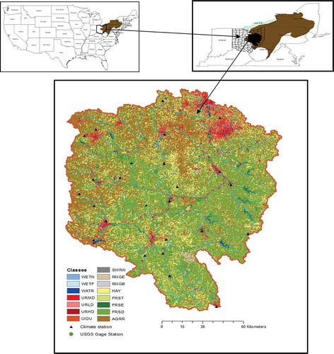
This research was conducted on the Muskingum watershed (Fig. 1), which is located in the eastern part of Ohio, USA. It covers an area of more than 20 720 km², which is nearly 20% of the State of Ohio. The Muskingum is the largest river in the watershed; it originates at the union of the Tuscarawas and Walhonding rivers near Coshocton and eventually drains into the Ohio River at Marietta. The main tributaries of this river are the Tuscarawas, Walhonding and Licking rivers and Wills Creek. The Muskingum watershed is a HUC-4 watershed (0504), which is subdivided into six HUC-8 watersheds: Licking (05040006), Walhonding (05040003), Mohican (05040002), Tuscarawas (05040001), Wills (05040005) and Muskingum (05040004). The Muskingum watershed contains nearly 19% of Ohio’s wetlands and 28% of the state’s lakes and reservoirs (Auch 2013).

Figure 1. Location map with climate and USGS stations in the Muskingum watershed. WETN: herbaceous wetland; WETF: wetland forest; WATR: open water; URMD: urban medium density; URLD: urban low density; URHD: urban high density; UIDU: industrial; SWRN: bare rock or sandy or clays; RNGE: grassland; RNGB: shrubland; HAY: hay; FRST: mixed forest; FRSE: evergreen forest; FRSD: deciduous forest; and AGRR: agriculture.

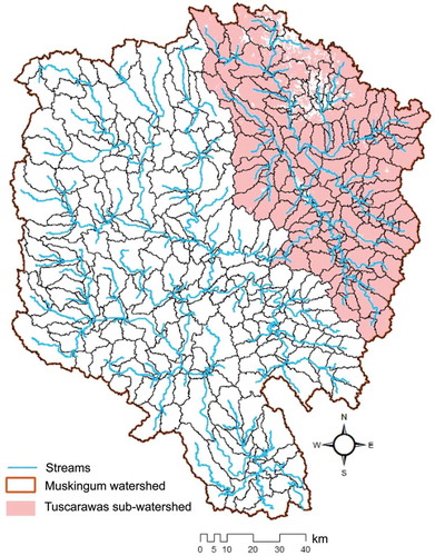
Utica Shale in eastern Ohio has great potential for the production of natural gas and oil. Currently, most of the unconventional natural gas wells in Ohio lie in the Muskingum watershed (Fig. 2). Several drilling companies are advancing in Ohio for oil and gas development and drilling has increased tremendously on this watershed. Most of the wells are concentrated on the eastern portion of watershed, the Tuscarawas sub-watershed, which covers an area of 6327 km² within the Muskingum watershed (Fig. 3). This sub-watershed covers all or partial areas of the 13 counties of Ohio. The northern portion of this sub-watershed is significantly covered by industrial and urban land uses, whereas the southern portion is dominated by forest cover. Additionally, there are several reservoirs in the eastern part of the watershed that are used for municipal water supplies.

Figure 2. Utica shale wells in the State of Ohio, USA, from January 2011 to September 2013, indicating more wells in Eastern Ohio.

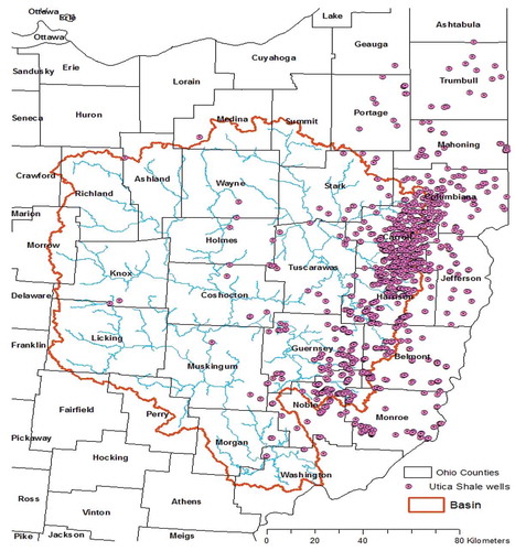
Figure 3. Tuscarawas sub-watershed (shaded) in the upper part of the Muskingum watershed, where drilling for hydraulic fracking has been increasing significantly.

SWAT model input

The DEM of 30 m resolution was downloaded from USGS National Elevation Dataset in order to delineate stream networks using ArcGIS, resulting in 406 sub-basins. Similarly, land-use data of 30 m resolution were downloaded from the National Land Cover Database 2006 to best represent the land-use pattern within the calibration period (2002–2009) of this model. The watershed comprised forest (47%), agricultural land with row crops (23%), hay (19%), and urban areas (10%). The remaining 1% of land use includes industrial areas, water, range grass and forested wetlands. The existing 12 reservoirs were spatially located manually at the proper locations of the watershed with reference to the stream outlet. The soil data taken from the State Soil Geographic dataset (STATSGO) (USDA 1991) were included as a default option in SWAT with a map at 1:250 000 scale. The appropriate number of HRUs (6176) was obtained by assigning multiple HRUs for each sub-basin in order to account in detail for the complexity of the landscape. This large number of HRUs was achieved despite eliminating minor land uses, soils and slopes by selecting thresholds of 5%, 15% and 15%, respectively. The large number of HRUs was highly beneficial for accurate prediction of streamflows (Arnold et al. 1996).

Seventeen years of climate data, including precipitation and the maximum and minimum temperature, were downloaded from the National Climatic Data Center (NCDC) website. Altogether, 23 precipitation stations and 19 temperature gauge stations were located within the watershed (Fig. 1). The remaining meteorological time series inputs, such as solar radiation, wind speed and relative humidity, were available from the SWAT model’s built-in weather generator. The daily streamflow data needed for model calibration and validation were available from the USGS website for nine USGS gauging stations from 1993 to 2009 (Fig. 1). The reservoir daily mean outflow data were available from the US Army Corps of Engineers (USACE) for the same period.

Data on point source discharges greater than 1890 m³/d were collected from the Ohio Environmental Protection Agency (OEPA) and used as model inputs before calibrating the model. Similarly, other water use information was obtained from the Ohio Department of Natural Resources (ODNR) in order to adequately represent the watershed conditions before model calibration and validation. The consumption of water for hydraulic fracking was more significant than the consumption of water for agriculture during 2012. The surface water withdrawal in Muskingum watershed in 2012 was 334 m³/d for hydraulic fracking, 308 m³/d for golf course irrigation, 220 m³/d for agriculture and 716 m³/d for industry. Groundwater withdrawal for hydraulic fracking in the same year was small (1%) compared to surface water withdrawal.

Water withdrawal information was verified from ODNR and OEPA. Similarly, the locations of oil and natural gas wells and sources for freshwater withdrawals greater than 378 m³/d were collected from ODNR. The completed well data, freshwater required per well, and recycled water quantities were obtained from FracFocus, which is the national hydraulic fracturing chemical registry. A summary of input data required, sources and format is presented in Table 1.

Model calibration and validation

In order to reduce the uncertainty in model prediction, a hydrological model needs to be properly calibrated and validated (Engel et al. 2007). For this, SWAT-CUP (Abbaspour et al. 2007) was selected to calibrate the model parameters using streamflow time series at various locations using the SUFI-2 algorithm. The efficiency of SUFI-2 for large-scale modelling studies was suggested by Yang et al. (2008). Since model calibration is an iterative process of establishing the best agreement between simulated and observed data, 21 model parameters (not shown), as discussed in several earlier studies (Abbaspour et al. 1999, Abbaspour et al. 2007, Schuol et al. 2008, Yang et al. 2008, Faramarzi et al. 2009), were selected for model calibration and validation at various locations of the watershed.

The model simulations were run for 15 years using observed data at nine USGS stream gauge stations (Fig. 1) from 1995 to 2009, including the calibration and validation periods. A warm-up period of 2 years was used in order to minimize the effect of unknown initial conditions and stabilize the hydrological component of the model. The model was then calibrated at a daily time scale on data for nine different USGS stream gauge from 2002 to 2009. In the next step, validation of the model was performed on data from 1995 to 2001 using statistical criteria to measure the goodness of fit, such as the coefficient of determination (R²) (Krause et al. 2005), the Nash-Sutcliffe coefficient of efficiency (NSE) (Nash and Sutcliffe 1970) and percentage bias (PBIAS). Also, we compared the simulated and observed flows for less than 75 percentile low flows. For better assessment of the model, users can perform the full split-sample test, inverting the roles of the calibration and validation periods. A detailed description of the model evaluation criteria is not included in this paper. Readers can refer to Sharma et al. (2015) for additional information on model evaluation procedures.

Scenario analysis

The calibrated and validated SWAT model was integrated with water use and point source data in order to develop theoretically realistic scenarios with different rates of fracking development. The baseline, current and future scenarios were developed to assess the impact on water resources under various levels of fracking. The baseline scenario referred to the watershed conditions for 2012, with water consumption including public water supply, domestic, industrial and other water uses for irrigation, livestock, mining, power plants and point sources, but no hydraulic fracturing water use. The current scenario utilized watershed conditions in the year 2012, including the fracking withdrawal rate of 2012 in addition to other consumptive uses. As the fracking boom was just beginning in 2012, we only had 3 years of drilling data available for this study. The future scenario projected the current rate of development of natural gas in the Muskingum watershed up to year 2030, based on the recent drilling trends. However, drilling water demand was the only parameter changed and other consumptive use was considered constant in all the scenarios. The future scenario was divided into two separate scenarios with respect to temporal scale. The “future scenario on current climate period” was developed by simulating streamflows using the projected hydraulic fracking conditions of year 2030 but using current climate conditions (2012). Similarly, the “future scenario on future climate period” refers to the projected hydraulic fracking condition of the year 2030 simulated over a climate period of 30 years, which was generated based on historical climate records. Monthly consumptive water use was provided from the water use input file based on the removal of water from stream reaches, shallow aquifers, and reservoirs within the sub-basin.

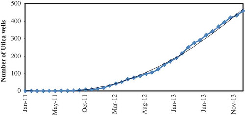
Since hydraulic fracking in Ohio is predominantly occurring in the eastern part of the state, detailed analysis for the future scenario was conducted for the Tuscarawas sub-watershed, as it covers the major eastern portion of the Muskingum watershed. Future fracking wells in the watershed (Fig. 4) were estimated based on the past 3 years of drilling trends in Ohio. Even though ODNR data reported that 865 wells were drilled in Ohio, drilling information on only 517 wells was available from FracFocus. Therefore, projections up to 2030 were based on actual wells drilled from FracFocus information. The future scenario was adopted with fracking wells increasing by 224 wells per month in Ohio by 2030. Even though the future trend of hydraulic fracking is uncertain and depends on many political and socio-economic constraints, we assumed that the extreme increase in fracking in the future scenario would provide an idea of the maximum environmental impact on stream low flows for policy makers. This study was motivated by the growing concern of communities and scientists about water resources availability in this region. The extreme worst-case scenario analysed for the future period was particularly important as an indicator of potential conflicts among water uses. The worst-case scenario refers to possible low flows due to the increased trend of fracking and impending drought.

Figure 4. Change in number of Utica wells in Ohio from January 2011 to May 2014.

A similar trend of hydraulic fracking as experienced in Ohio was assumed in the Tuscarawas sub-watershed. Sub-basins with a minimum net area of 2 km², after eliminating residential areas and water bodies, were used for analysis. This resulted in 149 out of 168 potential sub-basins being studied in this sub-watershed. The water withdrawal for each well was estimated based on water use trends in the Muskingum watershed for 2012 and 2013, available from FracFocus. The water use for each well in the Muskingum watershed was approximately 13 010 m³ in 2012 and 16 680 m³ in 2013 (Table 2). The freshwater withdrawal for each well was assumed to be 17 000 m³ in 2030 considering the similar past trend, drilling technology and conditions. The existing trends indicate a decreasing use of recycled water from 2012 (4.4%) to 2013 (3.8%); hence, recycled water for 2030 was considered simply as 4% of initial withdrawals. Water withdrawal was considered from multiple nearby sources such as the nearest streams and reservoir in the watershed, as suggested by Arthur et al. (2010). Water needed for fracking was used for 5–7 days (Sullivan et al. 2013). Generally, a density of one well per 4050 m² is considered for the development of shale wells (Myers 2009, Robbins 2013), and this information was used to determine the maximum possible limit on the number of wells in the watershed, resulting in 2030 wells on 149 sub-basins in the year 2030. These projected wells with consideration of 17 000 m³ of freshwater and 4% recycled water was equally distributed for each well for seven consecutive days in 149 sub-basins of Tuscarawas watershed. Later, this projected was considered with 30 years of plausible climate data in the SWAT model to simulate future scenarios. The future possible climate data were generated using a statistical downscaling model (SDSM) based on historical climate records of the region.

Table 1. Data used for SWAT model development in the Muskingum watershed.

Data type	Data	Source
GIS	30-m DEM	USGS National Geospatial Program (NGP) http://viewer.nationalmap.gov/viewer/
	Land use and land cover 2006	USGS National Geospatial Program (NGP), National Land Cover Dataset (NLCD), http://viewer.nationalmap.gov/viewer/
	Soil data	Geographic STATSGO soil map (scale of 1:250 000)
Climate	Rainfall and temperature	NOAA National Climatic Data Center (NCDC) http://www.ncdc.noaa.gov/cdo-web/
Hydrology	Streamflow	USGS http://waterdata.usgs.gov/usa/nwis/sw
	Reservoir outflow	US Army Corps of Engineers (USACE)
Stream networks/water bodies	Stream and flow direction, reservoirs	USGS National Geospatial Program (NGP) National Hydrograph Dataset (NHD)
Water use (surface and ground water)	Irrigation, public, power, mineral extraction, industries and golf courses	Ohio Department of Natural Resources (ODNR), Ohio Environmental Protection Agency (OEPA)
Point sources	Flow discharge	OEPA
Oil and natural gas	Wells for hydraulic fracking	ODNR
	Sources of drilling water	ODNR
	Drilling water estimate per well and future drilling trend	FracFocus (http://fracfocus.org) (National hydraulic fracturing chemical registry)

Table 2. Water withdrawal for hydraulic fracking per well in the Muskingum watershed, 2011–2013.

Year	Average vertical depth (m)	Freshwater (m^3)	Recycled water (%)
2011	7 720	11 450	13.8
2012	7 730	13 010	4.4
2013	10 900	16 680	3.7

Developing future climate

In this research, the SDSM tool was utilized to generate the future climate data by establishing the quantitative relationship between local surface variables (predictands) and large-scale variables (predictors). The National Center for Atmospheric Research (NCAR) and the National Centers for Environmental Prediction (NCEP) have developed more than 50 years of global analysis of atmospheric components. Therefore, these re-analysis data were selected to recover the missing measured data in the data assimilation system and make climate variables consistent throughout the re-analysis period. Large-scale predictors including mean temperatures, vorticity at surface and 850 hPa, zonal velocity and many more were selected from predictors obtained from NCEP/NCAR re-analysis data for the period 1961–1990, based on regression techniques (Table 3). Observed data from 1961 to 1975 were used to develop the regression model (calibration) and then regression weights produced a parameter file to validate for the period from 1976 to 1990. This process was repeated for all the precipitation stations. Once the missing data (1961–1990) had been infilled using a weather generator tool, the scenario generator from the SDSM was applied to generate precipitation. In order to generate a possible set of dry period precipitation, we used the historical set of observed precipitation and temperature data in the respective stations (23 precipitation and 11 temperature stations). The SDSM model was used to generate a possible set of future precipitation for a 30-year period. Since our intention was to run the model for a worst-case, low-flow scenario, we generated the 25th percentile precipitation datasets within the watershed at all stations.

Table 3. List of predictors used in the SDSM model to downscale the NCEP re-analysis data.

Station parameter	Predictor variable
Precipitation	Zonal velocity component at surface level
	Zonal velocity component at 850 hpa
	Geostrophic airflow velocity at 850 hpa
	Vorticity at surface level
	Vorticity at 850 hpa
	Sea level pressure
	Specific humidity at 500 hpa
	Specific humidity at 850 hpa
Temperature	Mean temperature
	Near surface specific humidity

Results

Model simulation

The model calibration and validation were performed on daily and monthly time scales. The model performance was satisfactory during the calibration and validation periods with reasonable accuracy, which was assessed through a visual inspection and statistical criteria. The daily and monthly statistical criteria measuring the performance of the model, NSE, R² and PBIAS, are listed in Tables 4 and 5, respectively. Analysis showed that NSE and PBIAS were satisfactory and mostly above the recommended ranges (Moriasi et al. 2007) (NSE > 0.5 and PBIAS ±25%) except at a few stations, especially for monthly simulation. The NSE values varied from 0.40 to 0.65 for both daily streamflow calibration and validation (Table 4). Similarly, the NSE varied from 0.49 to 0.89 for monthly streamflow calibration, and 0.55 to 0.86 for monthly streamflow validation (Table 5). The simulated streamflows slightly underestimated the daily and monthly peaks, which is consistent with previous findings (Bieger et al. 2014, Santhi et al. 2014). The mean observed and simulated low flows lower than the 75th percentile were compared with PBIAS (17%) and R² (0.78) (not shown). Overall, the model captured the temporal pattern of streamflow with reasonable accuracy.

Table 4. Statistical criteria measuring the daily performance of the SWAT model for the calibration (2002–2009) and validation (1995–2001) periods.

USGS gauge station	Calibration			Validation
	R^2	NSE	PBIAS (%)	R^2	NSE	PBIAS (%)
3117000	0.42	0.42	0	0.45	0.45	−2
3124500	0.43	0.40	−16	0.53	0.47	−10
3139000	0.51	0.49	−4	0.63	0.60	−3
3136500	0.47	0.46	9	0.41	0.40	18
3129000	0.57	0.56	3	0.54	0.47	21
3140500	0.63	0.63	2	0.69	0.65	12
3146500	0.42	0.40	11	0.43	0.42	12
3142000	0.55	0.47	13	0.51	0.49	−2
3150000	0.65	0.65	0	No data

Table 5. Statistical criteria measuring the monthly performance of the watershed model for the calibration (2002–2009) and validation (1995–2001) periods.

USGS gauge station	Calibration			Validation
	R^2	NSE	PBIAS (%)	R^2	NSE	PBIAS (%)
3117000	0.89	0.89	0	0.90	0.86	7
3124500	0.59	0.53	−16	0.63	0.61	−9
3139000	0.64	0.64	−4	0.72	0.71	−3
3136500	0.50	0.49	9	0.63	0.56	18
3129000	0.68	0.66	3	0.67	0.55	21
3140500	0.68	0.67	1	0.76	0.69	13
3146500	0.79	0.72	11	0.76	0.71	12
3142000	0.71	0.69	13	0.77	0.68	−1
3150000	0.73	0.72	0	No data

Table 6. Characteristics of the various scenarios used for analysis.

Scenario	Climate conditions	Hydraulic fracking
Baseline (without fracking) scenario	Current	No
Current (with fracking) scenario	Current	Yes
Future scenario on current climate period	Current	Projected fracking
Future scenario on future climate period	Future	Projected fracking

Scenario evaluation

Our earlier study (Sharma et al. 2015) analysed the impact of water withdrawal for the current conditions of hydraulic fracking, and found modest impact on 7-day low flows. The present study analysed the increasing drilling trend in the Muskingum watershed in order to determine the potential impact on environmental low flows and sustainable water availability for multiple uses. Low flows were evaluated for various fracking scenarios (Table 6); the results are described in the subsequent section.

Future and baseline scenario for current climate period

Sixteen sub-basins of increasing drainage area in the Tuscarawas watershed were selected to assess the impact of fracking on low flows at various locations. The analysis was accomplished by comparing the baseline scenario against the “future scenario on current climate period”, i.e. only changing the withdrawals due to fracking activities. Figure 5 shows the absolute change in the 7-day minimum flows between the baseline and future scenarios. Seven-day minimum flows were computed by the average flow measured during the seven consecutive days, and the minimum value from such a record was compared for baseline and future scenarios corresponding to various drainage areas. The link between the degree of impact of fracking and sub-basin size is presented in Fig. 6. This shows that the effect of withdrawal decreases with increase in the drainage area, and the minimum percentage difference is about 20%, which still represents a significant impact. Some outliers observed in the graph are mainly due to the interactions of other water use components and point sources on the same sub-basins. A difference of approximately 9% in annual average flow was predicted between the two scenarios (Fig. 7).

Figure 5. The 7-day monthly minimum flow during the low-flow period for baseline and future scenarios analysed for the current climate period in the Muskingum watershed.

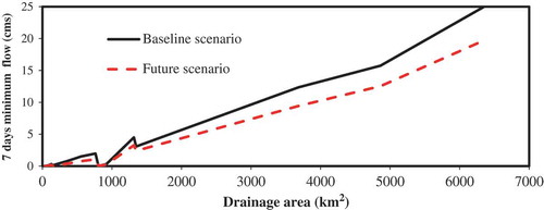
Figure 6. Percentage difference in 7-day minimum flows between the baseline and future hydraulic fracking scenarios simulated using current climate data in the Muskingum watershed.

Figure 7. Percentage difference in annual average flows between the baseline and future hydraulic fracking scenarios simulated using current climate data in the Muskingum watershed.

Future, baseline and current scenarios for future climate period

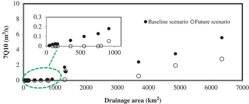
Environmental flow criteria were analysed, using a plausible set of generated climate data for sixteen similar sub-basins of the Tuscarawas watershed. These flow criteria were evaluated using DFLOW 3.1 (USEPA 2006) as a Windows-based tool, which was developed by the EPA. Figure 8 presents the comparison in 7Q10 between the baseline (without fracking) and future scenarios for the 30-year simulation period. Significant differences were detected under the future scenario compared with the baseline. The excess withdrawal due to future fracking reduced 7Q10 to zero for drainage areas of less than 800 km².

Figure 8. The 7Q10 flows for the baseline and future projected hydraulic fracking scenarios using the 30-year projected climate dataset generated by the SDSM.

Figure 9 shows the decreasing trend in the percentage difference in 7Q10 with increase in drainage area when the baseline scenario was compared with the future scenario. A relatively smaller difference was detected when analysis was conducted in a large drainage area. However, the percentage difference in 7Q10 remains significant (about 15%) even for the largest drainage areas considered. Additionally, comparisons between the baseline and future scenarios for 1B3 and 4B3 were performed on six different sub-basins, and also showed a similar decreasing trend. The difference in the 4B3 and 1B3 between the two scenarios is shown in Fig. 10. Figure 11 shows the decreasing trend in percentage differences in both criteria with increasing drainage area.

Figure 9. Percentage difference in 7Q10 between the baseline and projected future hydraulic fracking scenarios using the 30-year projected climate dataset generated by the SDSM.

Figure 10. The 4B3 and 1B3 flows for the baseline vs future fracking scenarios using the 30-year climate dataset generated by the SDSM.

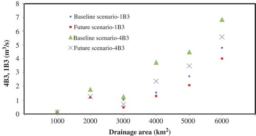
Figure 11. Percentage difference in 4B3 and 1B3 between the baseline and future hydraulic fracking scenarios using the 30-year climate dataset generated by the SDSM. The dotted line represents the trend in 4B3 and solid line represents the trend in 1B3.

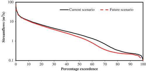
Analysis was also conducted to see the effect of the future scenario on the flow duration curve, as it is one of the important statistical tools used to quantify hydrological regimes (Kim and Kaluarachchi 2009). The 95 percentile flow exceedence was considered as the threshold for the extreme low flows, which indicates a stressful drought period as streams drop to the lowest level. Similarly, the 75 percentile flow exceedence was considered as low flow, which is the dominant low-flow condition sustained by the ground discharge into the streams. A sub-basin with a drainage area of 920 km² was selected to analyse the flow duration curve between the current and future scenarios for a period of 30 years (Fig. 12). The results showed that the high flow was not affected in this drainage area. However, the low flows were slightly affected as the alteration was noticed below 85% flow exceedence. The time series of the baseline, current and future scenarios depicts the visible change in the baseflow (not shown), indicating the impact of fracking withdrawals on flows in low-flow periods.

Figure 12. Flow duration curve for the current and future hydraulic fracking scenarios using the 30-year climate dataset generated by the SDSM in the Muskingum watershed.

Conclusions

In this paper, the impact of hydraulic fracking on water resources, especially during low-flow periods, was explored in the Muskingum watershed of Eastern Ohio, USA, considering the worst-case scenario. The SWAT watershed model was selected for the simulation of stream flows. The simulated flows at various locations were used to generate three scenarios that represent the range of potential impacts of water withdrawals for hydraulic fracking. The baseline scenario was based on realistic conditions of all water use data, but excluded withdrawals for fracking. The current scenario also used actual data for all water uses, including the present rate of water withdrawal for hydraulic fracking. The future scenario was modelled using 30 years of generated climate data based on the historical temperature and precipitation in the SWAT model. The SDSM was used to generate future temperature and precipitation based on the occurrence of the 25th percentile drier period precipitation in a 30-year period (1961–1990). Since we were not sure whether or not the highest temperature and precipitation would occur simultaneously, we simply used the generated temperature. The condition might be more critical if the lowest precipitation and highest temperature occurred simultaneously.

Seven-day low flows showed some variability when the baseline scenario was compared with the future projected scenario, indicating that flow alteration during low-flow periods might be an important consideration for regulation of water supply and quality. Simulations showed that 7Q10 could be reduced to zero for drainage areas of less than 800 km² due to projected future fracking activity. The percentage decrease in 7Q10 for larger drainage areas (>6000 km²) could be 15% or more. The difference due to fracking withdrawals was also noticeable on flow duration curves and baseflow time series, further reinforcing the potential impact of fracking during low-flow periods. Even mean annual flows were predicted to decrease by 9% or more under the future scenario.

It is important to note that the analysis was conducted using a worst-case scenario, assuming that fracking would continue to increase at the current trend. Based on the results of this study, we can conclude that the impact of hydraulic fracking may be very serious for headwater streams. Impacts on higher order streams will be less severe, but potentially significant enough to affect aquatic life, water quality and regulatory decisions.

The hydrological (7Q10) and biological (4B3 and 1B3) design streamflows in sub-basins of the Muskingum watershed were altered substantially, and in some cases (i.e. for headwater streams) dramatically, due to water withdrawal for hydraulic fracking in extreme scenarios. Therefore, it is essential that planners and decision makers account for water withdrawal for fracking while setting environmental flow criteria in NPDES permitting, particularly for headwater streams. This may prove challenging in a state such as Ohio, where different agencies issue permits for oil and gas drilling activities (ODNR) and wastewater discharges (OEPA).

Uncertainties exist in the complex watershed model associated with the input data, model development, future projected well drilling and water use, future advancement in drilling technology, climate, etc. However, this study has shown that modelling tools are available to estimate the impact of fracking withdrawals on streamflows and provide regulators with a better understanding of potential management options.

Acknowledgments

The authors are grateful for the suggestions made by the anonymous reviewers and the associate editor to improve this manuscript.

Disclosure statement

No potential conflict of interest was reported by the authors.

Additional information

Funding

We would like to acknowledge the United States Geological Survey/National Institutes for Water Resources (USGS/NIWR) for providing grant support through the Ohio Water Resources Center of the Ohio State University for this research work.

References

- Abbaspour, K.C., Sonnleitner, M.A., and Schulin, R., 1999. Uncertainty in estimation of soil hydraulic parameters by inverse modeling: example lysimeter experiments. Soil Science Society of America Journal, 63 (3), 501–509. doi:10.2136/sssaj1999.03615995006300030012x
- Abbaspour, K.C., et al., 2007. Modelling hydrology and water quality in the pre-alpine/alpine Thur watershed using SWAT. Journal of Hydrology, 333 (2), 413–430. doi:10.1016/j.jhydrol.2006.09.014
- Angle, M.A., Walker, D.D., and Jonak, J., 2001. Ground water pollution potential of Muskingum County, Ohio. Ohio Department of Natural Resources, Division of Water (No. 54), GWPP Report, 30–45.
- Arnold, J.G., et al., 1996. SWAT: soil and water assessment tool. User’s manual USDA agriculture research service grassland. Vol. 808. Soil and Water Research Laboratory, 190.
- Arnold, J.G., et al., 1998. Large area hydrologic modeling and assessment part I: model development1. Journal of the American Water Resources Association, 34 (1), 73–89. doi:10.1111/j.1752-1688.1998.tb05961.x
- Arthur, J.D., Uretsky, M., and Wilson, P., 2010. Water resources and use for hydraulic fracturing in the Marcellus shale region [online]. Available from: http://www. all-llc. com/publicdownloads/WaterResourcePaperALLConsulting.pdf [Accessed 11 November 2014].
- Auch, T., 2013. The Muskingum watershed and Utica shale water demands [online]. Available from: http://www.fractracker.org/2013/12/water-demands [Accessed 11 November 2014].
- Beaver, W., 2014. Environmental concerns in the marcelluai shale. Business and Society Review, 119 (1), 125–146. doi:10.1111/basr.2014.119.issue-1
- Bieger, K., Hörmann, G., and Fohrer, N., 2014. Simulation of streamflow and sediment with the soil and water assessment tool in a data scarce catchment in the three gorges region, China. Journal of Environment Quality, 43 (1), 37–45. doi:10.2134/jeq2011.0383
- Cothren, J., et al., 2013. Integration of water resource models with fayetteville shale decision support and information system. University of Arkansas and Blackland Texas A&M Agrilife, Final Technical Report.
- Craig, R.K., 2012. Hydraulic fracturing (Fracking), federalism, and the water-energy nexus. Idaho L. Rev., 49, 241.
- Engel, B., et al., 2007. A hydrologic/water quality model application protocol. Journal of the American Water Resources Association, 43 (5), 1223–1236. doi:10.1111/j.1752-1688.2007.00105.x
- Entrekin, S., et al., 2011. Rapid expansion of natural gas development poses a threat to surface waters. Frontiers in Ecology and the Environment, 9 (9), 503–511. doi:10.1890/110053
- Eslamian, S., ed., 2014. Handbook of engineering hydrology: fundamentals and applications. CRC Press.
- Faramarzi, M., et al., 2009. Modelling blue and green water resources availability in Iran. Hydrological Processes, 23 (3), 486–501. doi:10.1002/hyp.7160
- Gassman, P.W., et al., 2010. The worldwide use of the SWAT model: technological drivers, networking impacts, and simulation trends. In: 21st century watershed technology: improving water quality and environment conference proceedings, 21–24 February 2010, Universidad EARTH, Costa Rica. American Society of Agricultural and Biological Engineers, 1.
- Gregory, K.B., Vidic, R.D., and Dzombak, D.A., 2011. Water management challenges associated with the production of shale gas by hydraulic fracturing. Elements, 7 (3), 181–186. doi:10.2113/gselements.7.3.181
- GWPC and ALL Consultant, 2009. Modern shale gas development in the United States: a Primer. US Department of Energy, Office of Fossil Energy.
- Hubbert, M.K. and Willis, D.G., 1972. Mechanics of hydraulic fracturing. Washington, DC, 239–256.
- Kim, U. and Kaluarachchi, J.J., 2009. Climate change impacts on water resources in the Upper Blue Nile River Basin, Ethiopia. Journal of the American Water Resources Association, 45 (6), 1361–1378. doi:10.1111/j.1752-1688.2009.00369.x
- Krause, P., Boyle, D.P., and Bäse, F., 2005. Comparison of different efficiency criteria for hydrological model assessment. Advances in Geosciences, 5 (5), 89–97. doi:10.5194/adgeo-5-89-2005
- Montgomery, C.T. and Smith, M.B., 2010. Hydraulic fracturing: history of an enduring technology. Journal of Petroleum Technology, 62 (12), 26–40. doi:10.2118/1210-0026-JPT
- Moriasi, D.N., et al., 2007. Model evaluation guidelines for systematic quantification of accuracy in watershed simulations. Transactions of ASABE, 50 (3), 885–900. doi:10.13031/2013.23153
- Myers, T., 2009. Review and analysis of DRAFT supplemental generic environmental impact statement on the oil, gas and solution mining regulatory program well permit issuance for horizontal drilling and high-volume hydraulic fracturing to develop the marcellus shale and other low-permeability gas reservoirs.
- Nash, J. and Sutcliffe, J.V., 1970. River flow forecasting through conceptual models part I—A discussion of principles. Journal of Hydrology, 10 (3), 282–290. doi:10.1016/0022-1694(70)90255-6
- Neitsch, S.L., et al., 2005. SWAT theoretical documentation version 2005. Temple, TX: Soil and Water Research Laboratory.
- Nicot, J.P. and Scanlon, B.R., 2012. Water use for shale-gas production in Texas, US. Environmental Science & Technology, 46 (6), 3580–3586. doi:10.1021/es204602t
- Pyrce, R., 2004. Hydrological low flow indices and their uses. Watershed Science Centre, (WSC) Report (04–2004).
- Rahm, B.G. and Riha, S.J., 2012. Toward strategic management of shale gas development: regional, collective impacts on water resources. Environmental Science & Policy, 17, 12–23. doi:10.1016/j.envsci.2011.12.004
- Robbins, K., 2013. Awakening the slumbering giant: how horizontal drilling technology brought the endangered species act to bear on hydraulic fracturing. Case Western Reserve Law Review, 63 (4), 13–16.
- Rossman, L.A. and C. EPA, 1990. DFLOW user’s manual Cincinnati. Ohio: US Environmental Protection Agency, Risk Reduction Engineering Laboratory, 946–950.
- Santhi, C., et al., 2014. An integrated modeling approach for estimating the water quality benefits of conservation practices at the river watershed scale. Journal of Environmental Quality, 43 (1), 177–198. doi:10.2134/jeq2011.0460
- Satterfield, J., et al., 2008. Managing water resources challenges in select natural gas shale plays. In: Presented at the Ground Water Protection Council Annual Meeting, September, Chesapeake Energy Corp.
- Schuol, J., et al., 2008. Estimation of freshwater availability in the West African sub-continent using the SWAT hydrologic model. Journal of Hydrology, 352 (1), 30–49. doi:10.1016/j.jhydrol.2007.12.025
- Saunders, J.F., et al., 2004. The influence of climate variation on the estimation of low flows used to protect water quality: a nationwide assessment. Journal of the American Water Resources Association, 1339–1349. doi:10.1111/j.1752-1688.2004.tb01590.x
- Sharma, S., et al., 2012. Incorporating climate variability for point-source discharge permitting in a complex river system. Transactions of the ASABE, 55 (6), 2213–2228. doi:10.13031/2013.42507
- Sharma, S., et al., 2015. Hydrologic modelling to evaluate the impact of hydraulic fracturing on stream low flows using SWAT model: challenges and opportunities for simulation study. American Journal of Environmental Science, 11 (4), 199–215. doi:10.3844/ajessp.2015.199.215
- Sullivan, K., et al., 2013. Modeling the impact of hydraulic fracturing on drinking water resources based on water acquisition scenarios: phase 2. U.S. Environmental Protection Agency Office of Research and Development National Exposure Research Laboratory (NERL) Ecosystems Research Division (ERD) Athens, Georgia 30605 USA, 1 (1), 16–30.
- USDA (US Department of Agriculture), 1991. State soil geographic data base (STATSGO) data user’s guide. Miscellaneous publication, 1492.
- USEIA (US Energy Information Administration), 2011. Summary maps: natural gas in the lower 48 states [online]. Washington, DC. Available from: http://www.eia.gov/oil_gas/rpd/shale_gas.pdf [Accessed 26 July 2011].
- USEPA (US Environmental Protection Agency), 2012. Plan to study the potential impacts of hydraulic fracturing on drinking water resources: progress report. EPA/601/R-12/011.
- USEPA, 2006. DFLOW version 3.1 user’s manual. Washington, DC: U.S. Environmental Protection Agency, Office of Water.
- USEPA, 2011. Plan to study the potential impacts of hydraulic fracturing on drinking water resources. EPA/600/R-11/122.
- Vazquez-Amábile, G.G. and Engel, B.A., 2005. Use of SWAT to compute groundwater table depth and streamflow in the Muscatatuck River watershed. Transactions of the ASAE, 48 (3), 991–1003. doi:10.13031/2013.18511
- Wilby, R.L., Dawson, C.W., and Barrow, E.M., 2002. SDSM—a decision support tool for the assessment of regional climate change impacts. Environmental Modelling & Software, 17 (2), 145–157. doi:10.1016/S1364-8152(01)00060-3
- Wilby, R.L. and Dawson, C.W., 2013. Statistical downscaling model–decision centric (SDSM-DC) version 5.1 supplementary note. Loughborough: Loughborough University.
- Wiley, J.B., 2006. Low-flow analysis and selected flow statistics representative of 1930–2002 for streamflow-gaging stations in or near West Virginia. US Geological Survey.
- Yang, J., et al., 2008. Comparing uncertainty analysis techniques for a SWAT application to the Chaohe Watershed in China. Journal of Hydrology, 358 (1), 1–23. doi:10.1016/j.jhydrol.2008.05.012
- Yew, C.H. and Weng, X., 2014. Mechanics of hydraulic fracturing. Gulf Professional Publishing.