Development of RWQM1-based integrated water quality model in OpenMI with application to the River Zenne, Belgium

ABSTRACT

Descriptions of biochemical conversion processes based on QUAL principles have been used widely. We chose the recently developed IWA RWQM1 principles to model in-stream conversion of water quality components due to its sound physical background. An engine (a simulator) based on the RWQM1 principles was integrated with three other engine components—hydrological (SWAT), hydraulic (SWMM) and stream water temperature—in the OpenMI interface. We applied the integrated model to the River Zenne, Belgium. The results indicate that the integrated model can simulate various water quality components with a wide range of accuracy, from “Unsatisfactory” to “Very Good”. However, we could not validate the model against each of the RWQM1 components as most of the components were not measured in traditional river monitoring programmes.

KEYWORDS:

• River Zenne
• water quality
• QUAL
• RWQM1
• OpenMI

Editor M.C. Acreman; Associate editor not assigned

1 Introduction

Various engines (simulators) have been used for river water quality management. Engines, when populated with data, become models (OpenMI 2009), and are primarily used to explore the cause-and-effect relationship between an emission and its impact on the status of river water quality. They are also used to assess the effectiveness of implemented pollution regulation measures. At present, legislation and frameworks seem to drive water quality modelling (Reichert 2001). Such legislation in the European Union (EU) includes the Water Framework Directive (WFD; Council Directive 2000), which demanded mandatory improvement of the ecological status of water bodies by 2015. Since then, Belgium has made large investments for the proper management of wastewater, which have resulted in improved water quality for the River Zenne (Garnier et al. 2013). Despite these investments, the river still receives high loads of pollutants. As the river has a rather low discharge (around 10 m³/s on average), and large wastewater treatment plants (WWTP) discharge into the river (especially in Brussels), the water quality status of the river reaches in and downstream of Brussels is far from that required by the EU WFD. In this context, an inter-university, multidisciplinary research project “Good Ecological Status of the river Zenne (GESZ)” was launched, with the aim of evaluating the effects of alternative wastewater management plans on the ecological status of the river. This necessitated consideration of different processes such as: the hydrology of rural as well as urban catchments; hydraulics in the river, in sewer systems of the WWTPs and in the canal; soil erosion in upstream rural catchments and consequent transport in river reaches; nutrient cycling and transport; behaviour of toxic trace metals; and abundance of faecal bacteria.

Different processes need to be modelled, and many of the processes interact with each other, so integration of the models is needed. There is also growing consensus that real-world problems are complex and interrelated (Argent et al. 2006), and to solve them an integrated approach is a must (Parker et al. 2002, Candela et al. 2012, Bulatewicz et al. 2013). Further, the WFD also encourages practitioners to adopt an integrated approach. However, easy and feasible integration of different models is hindered because models are founded on different concepts, and have different spatial and temporal scales (Parker et al. 2002). In this context, the so-called “open-ended development” (Reichert et al. 2001a) or “open source route” (OpenMI 2009) is being increasingly sought, and recommendations towards “globally recognized standards and interface” are being made (Parker et al. 2002, Laniak et al. 2013). As such, the Open Modelling Interface or OpenMI (Moore and Tindall 2005, Gregersen et al. 2007) has emerged as one such “standard and interface” for model integration. Readers are referred to the papers of Bulatewicz et al. (2010), Betrie et al. (2011), Leta et al. (2011, 2012), Shrestha et al. (2012b, 2013, 2014M) and Leta (2014), among others, for uses of the OpenMI. The OpenMI allows an engine component that conforms to its standard to communicate during run time with other engine components (Moore and Tindall 2005, Gregersen et al. 2007). Furthermore, it is to be noted that the OpenMI is now an international Open Geospatial Consortium standard (OGC 2016), in fact the only recognized international standard for model linking.

Modelling of the nutrient cycle (carbon–nitrogen–phosphorus, C-N-P), also referred to more generally as river water quality modelling, is needed in the framework of integrated river basin management. In addition, the WFD classifies the ecological status of water according to the levels of various water quality variables (including C-N-P) and its possible impact on aquatic biota. In general, the use of traditional water quality models, such as that based on QUAL2E (of the US Environmental Protection Agency, US EPA)—an extended version of QUAL (Brown and Barnwell 1987)—is widespread. However, several researchers, e.g. Shanahan et al. (1998), Reichert et al. (2001a), van Griensven and Bauwens (2002), have pointed out the conceptual deficiency of the QUAL2E principles (see also Section 2.3 for details). The state variables of the formulation are different from the variables of activated sludge models (ASMs; Henze et al. 2000) for WWTPs, thereby hindering any possible integration with WWTP models. However, the principles of the recently formulated IWA River Water Quality Model No. 1 (RWQM1) address all the shortcomings of the QUAL2E formulation and hence have a solid physical background. Additionally, since the state variables of RWQM1 are similar to those of ASMs (for WWTPs), integration with the latter models is easier.

An engine based on the RWQM1 principles was integrated with three other engines: a hydrological engine, the Soil and Water Assessment Tool (SWAT; Arnold et al. 1998); a hydraulic engine, the Storm Water Management Model (SWMM; Rossman 2009); and a new stream water temperature engine in the OpenMI interface. We applied the integrated model to the River Zenne (Belgium) to simulate various water quality variables. The objectives of this work were to present new OpenMI-based developments and to test the RWQM1 formulation to simulate the water quality components of the River Zenne. Since SWAT employs the QUAL2E principles for the water quality conversion processes, and the new water quality engine is based on the RWQM1 principles, this paper also discusses the reconciliation issue between the two formulations.

2 Materials and methods

2.1 Study area

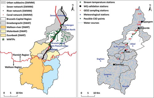
The River Zenne drains an area of 1162 km², has total length of about 103 km, and is crossed by a canal running parallel to the river (Fig. 1). The canal, upstream, is fed by former tributaries of the river. The canal also receives water from the river through several overflow structures. Downstream of Brussels, the excess water in the canal is discharged back into the river. About 1.5 million people live in the river catchment, of which about 70% live in Brussels alone (van Griensven 2002). There are several small to large WWTPs in the basin. The largest two are the Brussels-South WWTP, which treats about 360 000 equivalent-inhabitants (IE) and was put into operation in 2000, and the Brussels-North WWTP, which treats about 1.1 million IE and has been in operation since 2007.

Figure 1. (Left) The Zenne basin with the sub-basins simulated with SWAT, the SWMM network for the river, the canal, the sewer systems and the major WWTPs. (Right) The hydro-meteorological, stream temperature and water quality measurement stations, the GESZ sampling stations and possible combined sewer overflow (CSO) points.

2.2 River water quality modelling: a general concept

Somlyody and van Straten (1986) conceptualized a river water quality model as a structure having three axes. The first axis is time, and consequently the model can be dynamic and steady-state. The second axis is space, which is concerned with the number of (river) segments or boxes. The third component is ecological compartments (number of state variables of the water quality model). Hence, it is evident that there could be a large number of combinations. Accordingly, a large number of water quality models have been reported in the literature. Somlyody (1982) classified them into two broad classes: (a) transport oriented, in which emphasis is placed on hydrodynamic transport equations, and which describe transport and conversion of water quality variables in both space and time; and (b) ecologically oriented, in which emphasis is placed on biochemical conversion aspects, and hydrodynamic transport is simplified (or not even considered). A very similar classification is made by Watanabe et al. (1983) under “engineer-developed” and “biologist-developed” approaches. One such model combining both approaches in full three-dimensional form can be written as:

(1) $\frac{\delta c}{\delta t}=-u\frac{\delta c}{\delta x}-v\frac{\delta c}{\delta y}-w\frac{\delta c}{\delta z}+\frac{\delta }{\delta x}\left({\epsilon }_x\frac{\delta c}{\delta x}\right)+\frac{\delta }{\delta y}\left({\epsilon }_y\frac{\delta c}{\delta y}\right)+\frac{\delta }{\delta z}\left({\epsilon }_z\frac{\delta c}{\delta z}\right)+r\left(c,p\right)$(1)

where c is the concentration vector for n-state variables; t is the time; u, v and w, and ε_x, ε_y and ε_z are the velocity and diffusion coefficient components in the x, y and z coordinate directions, respectively; and r is the conversion rate of water quality (state) variables.

Equation (1) can be translated in that the change in the concentration is because of (a) physical transport processes and (b) biochemical conversion r (Somlyody and van Straten 1986, Reichert 2001). The parameters are subject to calibration. Physical transport processes need detailed information on the velocity components and diffusion coefficients. Input from a hydraulic model is thus needed to solve the equation. Equation (1) can be solved either numerically or using a conceptual approach. It should be noted that for all practical purposes Equation (1) is simplified. Solving the full set of Equation (1) numerically would require a high computation overhead, so conceptual approaches are becoming popular (Somlyody and van Straten 1986). One simplification would be a depth-integrated two-dimensional form of Equation (1). This is particularly valid when L_V (complete mixing in the direction of the depth of the river) is short, as is evident in very shallow rivers. Similarly, if the river length (L) is long compared with L_L (the distance of complete mixing over the entire cross-section), a further simplification can be made by integrating across the width (Reichert et al. 2001a), which can be written as (Somlyody and van Straten 1986):

(2) $\frac{\delta \left(Ac\right)}{\delta t}=-\frac{\delta \left(Qc\right)}{\delta x}+\frac{\delta }{\delta x}\left(A{D}_L\frac{\delta c}{\delta x}\right)+r\left(c,p\right)$(2)

where A is the cross-sectional area of the river; Q is the discharge in the river; and D_L is the longitudinal dispersion coefficient.

If we assume a total river length consisting of small river segments in which perfect mixing is said to be achieved, a further simplification can be made. In this case, Equation (2) reduces to an ordinary differential equation, which is easier to solve. In other words, it then conforms to continuous stirred tank reactor (CSTR) principles. In such an assumption, reality is indeed compromised, but there is widespread use of CSTR principles in the field of water and environmental disciplines (Peng 1994). However, it should be noted that such box models have conceptual deficiencies (Reichert et al. 2001a) and could have considerable effects on overall river dynamics (Krebs et al. 1999).

2.3 Evolution of conversion models

The history of representing biochemical conversion processes (r(c,p) in Equations (1) and (2)) dates back to 1925 (Reichert et al. 2001a). The pioneering work of Streeter and Phelps (1925) was the first of its kind. This classic model considers only two processes (biodegradation of organic matter and re-aeration) to compute the effect of organic waste disposal on the oxygen level fluctuations in a river. Since then, efforts have been made to include various other components. The most notable changes appeared in QUAL1 (Masch 1971) of the US EPA, in which a distinction was made between nitrogenous (NBOD) and carbonaceous (CBOD) biochemical oxygen demand, and nitrogen processes were incorporated. In the US EPA’s QUAL2, phosphorus processes and algae were added (Roesner and Evenson 1981), and this was later extended (for details, see Brown and Barnwell 1985). Later, improvement was made by incorporating the re-aeration effect of dams and the model was named QUAL2E-UNCAS (Brown and Barnwell 1987). Since then, the QUAL2 family of models has been so widely used that any new development (regarding biochemical process descriptions) should be examined taking the former as reference (Reichert et al. 2001a).

While the QUAL family models are widely used, various studies, e.g. Shanahan et al. (1998), Reichert et al. (2001a), van Griensven and Bauwens (2002), have highlighted their shortcomings, for example:

• QUAL family models assume BOD as a state variable; as a consequence, mass balance cannot be closed because BOD does not account for all biodegradable matter.

• Pelagic bacteria are not considered as a state variable, but their effect is considered in the form of a single biodegradation coefficient; as a result, consideration of population changes in the bacterial composition becomes impossible.

• QUAL2 family models cannot straightforwardly be integrated with WWTP models due to differences in model components.

In order to formulate a better conceptual framework for water quality modelling in riverine environments, the International Water Association (IWA) established a task group on river water quality modelling (Reichert et al. 2001b). The task group addressed the shortcomings of previous water quality models, especially that of the QUAL family models, and made sure that a new model could straightforwardly be linked to ASMs. The latter requirement was important because environmental modelling practitioners needed integrated modelling. Integrating ASMs and river water quality models was not straightforward as both models considered different state variables. However, it should be noted that there had been some efforts to reconcile them, such as by Masliev et al. (1995) and by Marijns and Bauwens (1997). The task group came up with a new river water quality model: the RWQM1 (see Section 2.4.3). Since its formulation, this model has been used in its original (or reduced) form (Borchardt and Reichert 2001, Reichert 2001, Martín et al. 2006), or in modified form (van Griensven and Bauwens 2002, Broekhuizen et al. 2012). The formulation has its roots in the ASMs for WWTPs and can be seen as “cross-fertilization” of ASM and river water quality models at that time.

2.4 Engines of the integrated model

In the following sections, we use specific terminology, as suggested by the OpenMI Association (OpenMI 2009), such as engine: “a generic representation of a process and this is where the calculations for simulating or modelling that process take place” (OpenMI 2009), model: “when an engine has read its input it becomes a model” (OpenMI 2009), and so on. The term “simulator” is often used synonymously for “engine”, which is also used in this article.

When selecting engines for integrated modelling, we opted for open-source engines that had been successfully applied in similar catchments. Owing to the nature and complexity of the River Zenne, we selected the SWAT engine for the simulation of the predominantly upstream river basin. As the river experiences backwater effects and tidal effects at downstream reaches, and there are complex interactions between the river, the sewer systems and the canal through various hydraulic structures, SWAT is not suitable for the middle and lower reaches of the river. Hence, we selected SWMM as the hydraulic engine. Furthermore, additional engines for the stream water temperature and water quality conversion were needed because SWMM does not have a robust water quality engine, and the kinematic parameters of any water quality engine are highly temperature dependent. In the following sections, the different engines are briefly described. However, emphasis is put on the water quality conversion engine that is the focus of this paper.

2.4.1 Hydrological engine

The SWAT model is a hydrological engine that can perform long-term continuous simulation of a variety of processes on user-specified time steps. The hydrological response units (HRUs) are the spatial entities of the engine; they are aggregated to sub-basins, and the sub-basins are further aggregated to a watershed (Arnold et al. 2011).The water quality conversion engine of SWAT is based on the QUAL2E formulation (Brown and Barnwell 1987). The formulation considers nine components and 15 processes (the Table 1). We refer readers to Arnold et al. (2011) for further details regarding the SWAT engine.

Table 1. Stoichiometric matrix with process rates of the QUAL2E formulation.

Component	1	2	3	4	5	6	7	8	9
Process	DO	BOD	ABM	ORG-N	NH4	NO2	NO3	ORG-P	DIS-P	Process rate
1. Re-aeration	1									K2.(DOsat- DO)
2. Biodegradation	−1	−1								K1.BOD
3. BOD sedimentation		−1								K3.BOD
4. Sediment DO demand	−1									K4/d
5. Photosynthesis	α3		1		−0.07.FNH4		−0.07.(1-FNH4)		−0.01	μmax.ABM.F(L,N,P)
6. Respiration	−α4		−1	0.07				0.01		ρ.ABM
7. Algae sedimentation			−1							σ1/d.ABM
8. Nitrogen hydrolysis				−1	1					β3.ORG-N
9. Nitrification 1st step	−3.43				−1	1				β1.NH4.f(DO)
10. Nitrification 2nd step	−1.14					−1	1			β2.NO2.f(DO)
11. N sedimentation				−1						σ4.ORG-N
12. N sediment release					1					σ3/d
13. P hydrolysis								−1	1	β4.ORG-P
14. P sedimentation								−1		σ5.ORG-P
15. P sediment release									1	σ2/d

DO: dissolved oxygen; BOD: biochemical oxygen demand; ABM: algal bio-mass; ORG-N: organic nitrogen; NH4: ammonium nitrogen; NO2: nitrite nitrogen; NO3: nitrate nitrogen; ORG-P: organic phosphorus; DIS-P: dissolved phosphorus; K1: de-oxygenation coefficient; K2: re-aeration coefficient; K3: BOD settling rate; K4: sediment oxygen demand rate; d: mean stream depth; μmax: maximum algal growth rate; ρ: algal respiration rate; σ1: algal settling rate; σ2: benthic source rate for P; σ3: benthic source rate for N; σ4: N settling rate; σ5: P settling rate; β1: ammonia oxidation rate; β2: nitrite oxidation rate; β3: N hydrolysis rate; β4: P hydrolysis rate; α3: oxygen production rate per unit of algal growth; α4: oxygen uptake per unit of algal respiration; f(L,N,P): algal growth limitation factor; f(DO): nitrification limitation factor; FNH4: ammonia preference factor.

2.4.2 Hydraulic engine

The SWMM model is a hydraulic engine that can be used for single-event or continuous dynamic rainfall–runoff simulation. SWMM can compute runoff quantity and quality, especially from urban areas (Rossman 2009). Like SWAT, SWMM can compute various components of the hydrological cycle. It employs the full set of Saint Venant equations (Lai 1987) to route runoff from the sub-catchments. SWMM does not have a conventional, straightforward engine for water quality conversion processes. However, users can define a pollutant, and theoretically it is possible to write an expression in terms of hydraulic variables (depth, volume, hydraulic residence time, etc.) that could mimic the conversion sought. Hence, it was felt that a new water quality conversion engine needed to be developed to complement the SWMM engine. We refer readers to Rossman (2009) for further details regarding the SWMM engine.

2.4.3 Water quality engine

As mentioned in Section 2.2, changes in concentration, c, of a water quality variable are due to conversion and transport processes (advection and dispersion). We used the RWQM1 formulation to represent the water quality conversion processes—r(c,p) in Equation (1)—by considering 30 processes (Table 2) and 24 components.

Table 2. Stoichiometric matrix with process rates of the RWQM1 formulation. All the non-zero positive stoichiometric coefficients are given a + sign. Similarly, − denotes a negative coefficient, and ? denotes coefficients whose sign depends on the composition of organic substances involved in the process. + is the same as ? but, in this case, the composition of compounds and stoichiometric parameters should be chosen in such a way that the resulting coefficient is always non-negative.

Component → i		1	2	3	4	5	6	7	8	9	10	11	12	13	14	15	16	17	18	19	20	21	22	23	24
j	Process ↓	SS	SI	SNH4	SNH3	SNO2	SNO3	SHPO4	SH2PO4	SO2	SCO2	SHCO3	SCO3	SH	SOH	SCa	XH	XN1	XN2	XALG	XCON	XS	XI	XP	XII
1a	Aerobic growth of heterotrophs with NH4	−		?				?		−	+			?			1
1b	Aerobic growth of heterotrophs with NO3	−					−	?		−	+			?			1
2	Aerobic respiration of heterotrophs			+				+		−	+			−			−1						+
3a	Anoxic growth of heterotrophs with NO3	−				+	−	?			+			?			1
3b	Anoxic growth of heterotrophs with NO2	−				−		?			+			?			1
4	Anoxic respiration of heterotrophs			+			−	+			+			−			−1						+
5	Growth of 1st stage nitrifiers			−		+		−		−	−			+				1
6	Aerobic respiration of 1st stage nitrifiers			+				+		−	+			−				−1					+
7	Growth of 2nd stage nitrifiers					−	+	−		−	−			−					1
8	Aerobic respiration of 2nd stage nitrifiers			+				+		−	+			−					−1				+
9a	Growth of algae with NH4			−				−		+	−			−						1
9b	Growth of algae with NO3						−	−		+	−			−						1
10	Aerobic respiration of algae			+				+		−	+			−						−1			+
11	Death of algae			(+)				(+)		(+)	?			?						−1		+	+
12a	Growth of consumers on XALG			(+)				(+)		−	?			?						−	1	+
12b	Growth of consumers on XS			(+)				(+)		−	?			?							1	−
12c	Growth of consumers on XH			(+)				(+)		−	?			?			−				1
12d	Growth of consumers on XN1			(+)				(+)		−	?			?				-			1
12e	Growth of consumers on XN2			(+)				(+)		−	?			?					−		1
13	Aerobic respiration of consumers			+				+		−	+			−							−1		+
14	Death of consumers			(+)				(+)		(+)	?			?							−1	+	+
15	Hydrolysis	+		(+)				(+)		(+)	?			?								−1
16	Equilibrium CO2↔HCO3										−1	1		+
17	Equilibrium HCO3↔CO3											−1	1	+
18	Equilibrium H2O↔H + OH													1	1
19	Equilibrium NH4↔NH3			−1	1									+
20	Equilibrium H2PO4↔HPO4							1	−1					+
21	Equilibrium Ca↔CO3													+		1
22	Absorption of phosphate							−1																1
23	Desorption of phosphate							1																−1

S_S: dissolved organic substances; S_I: inert dissolved organic substances; S_NH4: dissolved NH₄; S_NH3: dissolved NH₃; S_NO2: dissolved NO₂; S_NO3: dissolved NO₃; S_HPO4: part of inorganic dissolved phosphorus; S_H2PO4: part of inorganic dissolved phosphorus; S_O2: dissolved oxygen; S_CO2: sum of dissolved carbon dioxide and carbonic acid; S_HCO3: dissolved bicarbonate; S_CO3: dissolved carbonate; S_H: dissolved hydrogen ions, the pH can then be calculated as −log(S_H); S_OH: hydroxyl ions; S_Ca: dissolved calcium; X_H: heterotrophic organisms; X_N1: organisms oxidizing ammonia to nitrite; X_N2: organisms oxidizing nitrite to nitrate; X_ALG: algae and microphytes; X_CON: consumers; X_S: particulate organic materials; X_I: inert particulate organic matter; X_P: inert phosphate, phosphate adsorbed to particles; X_II: inert particulate inorganic material.

The complexity of the RWQM1 formulation is due to the fact that it has 36 kinetic parameters, 6 equilibrium parameters, 13 stoichiometric parameters and 36 mass fractions when considering only the water column (Reichert et al. 2001b). For rivers, where sediment plays an important role in nutrient conversion, the sediment compartment should be considered explicitly (Vanrolleghem et al. 2001). This complexity is cited by Marijns and Bauwens (1997) as the biggest disadvantage of the formulation. For the purposes of clarity, we do not present all the process rates and stoichiometric coefficient equations. Readers are thus referred to Reichert et al. (2001b).

In our current implementation, we considered the water column only and the processes therein. Re-aeration is considered as a boundary term at the air–water interface, with the process rate the same as that of QUAL2E (Table 1). Similarly, weir re-aeration is considered and calculated as:

(3) $r_{\mathrm{d}}=1+0.38\hspace{0.17em}ab\mathrm{\Delta }h\left(1-0.11\mathrm{\Delta }h\right)\left(1+0.046T_{\mathrm{s}}\right)$(3)

where r_d is the ratio of the oxygen deficit upstream and downstream of the weir; a is the water quality coefficient; b is the weir coefficient; ∆h is the water level difference between the upstream and downstream sides of a dam; and T_s is the stream water temperature (see Section 2.4.4 for details on how T_s should be calculated).

To calculate the electrical conductivity (EC, μS/cm), we considered five extra variables: (a) S_K: dissolved potassium, (b) S_Na: dissolved sodium, (c) S_Mg: dissolved magnesium, (d) S_Cl: dissolved chloride and (e) S_SO4: dissolved sulphate. These variables, however, are not subject to any conversion. We first calculated the total dissolved substances (TDS, in mg/L) as the sum of these extra variables along with S_HCO3, S_NH3 + S_NH4, S_NO2+ S_NO3, S_HPO4 + S_H2PO4 and S_Ca, and converted to EC using a conversion coefficient K, which is taken as 0.69 (mg/L)/(μS/cm), a value adopted from the study of Verbanck (1995) in a similar system. Temperature dependence on electrical conductivity was calculated based on observation made by Hayashi (2004) and given as:

(4) $\mathrm{E}{\mathrm{C}}_{T_{\mathrm{s}}}=\mathrm{E}{\mathrm{C}}_{{25}^{\circ }\mathrm{C}}\hspace{0.17em}\left(1+0.00187\left(T_{\mathrm{s}}-25\right)\right)$(4)

where EC_Ts is the electrical conductivity at T_s, and EC_25°C is the electrical conductivity at 25°C.

As the water quality model complements the SWMM model (see Section 2.5 for details), the advection of the water quality variables is based on the Saint Venant equations. However, we neglected the dispersion and subsequently used CSTR principles. We are aware of the limitations of such a simplification. Our choice was driven by the broad objectives of the GESZ project, which is the evaluation of various management plans in the ecological functioning of the river. This essentially requires continuous, long-term simulation to consider different conditions (dry and wet) of the river (Demuynck et al. 1997). Hence, we needed an engine that has a sound physical background and is computationally fast. The engine may not replicate a single event with very high accuracy, but it should represent the basin processes in a rather more coherent way.

2.4.4 Temperature engine

The kinematic parameters of the RWQM1 conversion engine are temperature dependent (Reichert et al. 2001b) and should duly be compensated for temperature. Hence, the conversion engine should be coupled with a temperature engine. To simulate the stream water temperature (T_s), as the air temperature data (T_a) are more readily available, we used a regression model between T_a and T_s. Of the various forms of regression equation, we used a nonlinear one (Equation (5)), as proposed by Mohseni et al. (1998). As several studies, e.g. Grant (1977) and Stefan and Preud’homme (1993), have shown, the typical time lag between T_s and T_a is 2 days, so this study used a time lag of 2 days. Moreover, we also considered thermal discharges (e.g. from the WWTPs) as they would influence the stream water temperature in reaches immediately downstream of the discharge point.

(5) $T_{\mathrm{s}}=\mu +\frac{\alpha -\mu }{1+{\mathrm{e}}^{\gamma \left(\beta -T_{\mathrm{s}}\right)}}$(5)

where μ and α are the minimum and maximum stream temperatures (°C); γ is the steepest slope at the inflection point of T_s versus T_a (–); and β is the air temperature at the inflection point of the same plot (°C).

2.5 Engine components on the OpenMI interface

The two engines SWAT and SWMM were migrated to the OpenMI interface. We refer readers to Shrestha et al. (2012a) for details on SWMM–OpenMI migration. For SWAT–OpenMI migration, we upgraded the work of Betrie et al. (2011), incorporating changes in the latest version of the SWAT engine. We coded the new engines (temperature and water quality) to make them directly OpenMI-compliant. As such, these (new) engines use the SWMM project to get the node and link characteristics, thereby carrying out simulation over the same river trajectory as in the SWMM project. The new engines use hydraulic variables such as velocity and water depth from the SWMM simulation. As such, a significant part of the code base is common, and these are indeed shared and not duplicated with the help of class hierarchy—the GESZ.SWMMNetwork (see Fig. 2).

2.6 Model build-up, inputs, calibration and validation

Table 3 shows various data used for the build-up, calibration and validation of the models. While flow and hydro-meteorological data were monitored on an hourly or daily basis, physicochemical data were monitored only once a month. The data from the major WWTPs in Brussels before 2007 were not usable as these WWTPs were not fully functioning then. A series of sampling campaigns was therefore set up during the GESZ project. These included (a) five campaigns (in different seasons) during dry weather conditions (DWFs) and (b) two campaigns during storm conditions (which included a 24-hour campaign). We therefore derived some variables/parameters from the GESZ sampling campaigns, then calibrated and validated the models based on the observed time series data of various physiochemical variables made available by different agencies.

Table 3. Model inputs of different components of the integrated water quality model.

Input	Value/Resolution	Remarks/References
(A) SWAT
(a) Digital elevation model (DEM)	30 m × 30 m	ASTER GDEM^1, DHM-OC GIS Vlaanderen
(b) Soil map	20 m × 20 m	Carte Numérique des Sols de Wallonie (CNSW)^2, VLM-OC GIS Vlaanderen
(c) Land-use map	20 m × 20 m	Corrine (Walloon region), VLM-OC GIS Vlaanderen
(d) Hydro-meteorological data (rainfall, relative humidity, wind speed, solar radiation, temperature)	Daily	Royal Meteorological Institute of Belgium (RMI), Direction Générale opérationnelle de la mobilité et des Voies Hydrauliques (DGVH)^3, Vlaamse Milieumaatschappij (VMM)^4
(e) Fertilizer application	Seasonal^5	Direction Générale Opérationnelle Agriculture, Ressources Naturelles et Environnement (DGARNE)^6, Vlaamse Landmaatschappij (VLM)^7
(f) Point sources	Yearly/constant	Société Publique de la Gestion de l’Eau (SPGE)^8
(B) SWMM
(a) River/canal longitudinal profile and cross-section geometry	approx. 100 m	Waterbouwkundig Laboratorium^9
(b) River longitudinal profile and cross-section geometry	approx. 100 m	Waterbouwkundig Laboratorium^9
(c) WWTP-Brussels-North sewer system geometry	approx. 100 m	Translated from a hydraulic model HYSTEM-EXTRAN built by Department of Hydrology and Hydraulic Engineering, Vrije Universiteit Brussel
(d) Rainfall	Hourly	Royal Meteorological Institute of Belgium (RMI)^10, Société Bruxelloise de Gestion de l’Eau/Brusselse Maatschappij voor Waterbeheer (SBGE/BMWB)^11
(e) Tide levels at outlet	30 min	Waterbouwkundig Laboratorium^9
(f) Boundary flows at tributaries	Daily	SWAT simulated
(C) Temperature model
(a) Air temperature	Daily	Royal Meteorological Institute of Belgium (RMI)^10
(b) Temperature of WWTP effluent	20°C	Constant (based on GESZ measurements)^12
(c) Temperature of CSO points	15°C	Constant (assumed)
(D) Water quality model
(a) Water quality variables at tributaries	Daily	SWAT simulated
(b) WWTP Brussels-North	Daily	Aquiris^13,*
(c) WWTP Brussels-South	Daily	Vivaqua^14,*
(d) Other WWTPs	Weekly	Aquafin^15,*
(e) Water quality concentration at CSO points	–	Constant (based on GESZ measurements)^12
(f) Water quality concentration at river outlet	–	Constant (based on GESZ measurements)^12

¹http://www.gdem.aster.ersdac.or.jp/search.jsp; ²http://cartographie.wallonie.be/NewPortailCarto/; ³http://voies-hydrauliques.wallonie.be; ⁴http://www.hydronet.be; ⁵Considered to be typically applied from February to August of every year; ⁶http://environnement.wallonie.be/; ⁷http://www.vlm.be/; ⁸http://www.spge.be/; ⁹http://www.watlab.be/nl; ¹⁰http://www.meteo.be/meteo/view/en/65239-Home.html; ¹¹http://www.sbge.be/; ¹²GESZ measurement: observed during GESZ sampling campaigns at different stations (Fig. 1, right); ¹³http://www.aquiris.be/; ¹⁴http://www.vivaqua.be/; ¹⁵http://www.aquafin.be/nl/; *Not all the variables of the RWQM1 are measured. Constant values of other variables measured during the GESZ sampling campaign are therefore used.

2.6.1 SWAT model for the Walloon region

The SWAT engine is the first engine component of the integrated modelling chain (Fig. 3); therefore, it does not require data input from any other models. Hence, we built, calibrated and validated it as a standalone engine.

Figure 2. The OpenMI wrapper design showing shared (static) SWMM network with two new components: temperature and water quality.

Figure 3. The different components in the integrated model and the data flow.

The engine required three spatial datasets: (a) elevation, for which we used a SWAT 30 m × 30 m digital elevation model (DEM) obtained from the ASTER-GDEM; (b) a soil map (20 m × 20 m) obtained from a government agency (Table 3); and (c) a land-use map (20 m × 20 m) obtained from a government agency (Table 3). Daily meteorological data, such as rainfall, temperature, relative humidity, solar radiation and wind speed, were enforced in the model. Based on the spatial data, the watershed was disaggregated into 30 sub-basins and 234 HRUs.

The SWAT model (after the engine had been populated with data) was simulated for the years 1988–2010 and this was later split such that the years 1998–2008 were used for calibration and 1988–1997 and 2009–2010 for validation. We used a station named Tubize (Fig. 1) to evaluate the model performance on a daily time scale (see Leta et al. (2011, 2012) for further information).

For water quality variables, due to data limitations, we were forced to use the years 1998–2008 for calibration, and 1994–1997 and 2009/10 for validation. As such, five water quality variables (DO, BOD, NH₄, NO₃ and DIS-P) measured at Quenast (Fig. 1) were used. The water quality parameters (kinetic and stoichiometric) were optimized using a heuristic approach. For this, the range of parameter values provided by Brown and Barnwell (1987) was respected.

2.6.2 SWMM model

We implemented four sub-systems of the basin in the SWMM model: (a) the river downstream of the border with the Flemish region of Walloon (Wallonia) (Fig. 1); (b) the canal, including the exchange points with the river; (c) the sewer systems of the WWTPs including the combined sewer overflows (CSO) point; and (d) the urbanized catchment in and around Brussels.

The implementation of the SWMM system required longitudinal and cross-sectional geometrical data, as well as supplying meteorological data (e.g. daily rainfall and temperature) and measured daily evaporation time series (Table 3). The implementation of the SWMM system resulted in about 2400 nodes (and links) and 180 special structures, including weirs, orifices, pumps and storage units.

As shown in Figure 3, the SWMM engine requires rural catchment runoff as simulated by the SWAT engine; therefore, we integrated SWAT and SWMM engine components in the OpenMI, which involved the exchange of “streamflow” from SWAT to SWMM.

We used observed streamflow (daily and hourly) of the year 2007/08 at three locations, namely, Lot, Vilvoorde and Eppegem (Fig. 1), to calibrate and of 2009–2010 to validate the integrated (SWAT-SWMM) model.

2.6.3 Temperature model

We used T_a recorded at Ukkel (Fig. 1) and T_s at four locations upstream of Brussels to optimize the parameters of the adopted regression equation. We then set up an integrated temperature model that included SWAT, SWMM and the temperature engine components. For this, constant temperatures of 20°C for WWTP effluents and 15°C for CSOs were assigned as thermal sources. The constant value (15°C) was an estimate based on the measurements in GESZ sampling campaigns (Table 3). We validated the simulated T_s at three stations, namely, Lot, Vilvoorde and Eppegem for the years 2007–2010.

2.6.4 Integrated water quality model

As a final step, an integrated water quality engine consisting of SWAT, SWMM, the temperature and the water quality engines was set up (Fig. 3). Figure 3 also shows the different data that are exchanged between the engines, associated element sets and the time steps involved.

As stated previously, the sampling frequency of the water quality variables by the different agencies was once per month, which made the task of (integrated) model build-up, calibration and validation rather difficult. An additional problem was related to the use of the RWQM1 formulation for modelling the water quality conversion processes. Some components of the formulation (e.g. microbial biomasses) are not generally included in traditional river monitoring programmes (van Griensven and Bauwens 2002). Even for the components that are generally included in river monitoring, no measurements were recorded in extreme conditions.

The water quality engine also required the daily SWAT simulated water quality variables from rural catchments (Fig. 3). However, the linking is not straightforward, as the SWAT water quality engine is based on QUAL2E, while the new water quality engine employs RWQM1 conversion model principles. Some components of the two conversion engines, such as NH₄ → S_NH4 (Tables 1 and 2), are identical and therefore directly compatible, while others are not. Components such as bacterial biomass (X_H, X_N1, etc.) are not considered in the QUAL2E formulation. The organic pollution in QUAL2E is represented as BOD, while RWQM1 divides the organic matter into four classes, namely S_S, S_I, X_S and X_I (Table 2). To calculate the organic fractions and bio-masses coming from the upstream boundaries, BOD (simulated by SWAT) can first be converted to chemical oxygen demand (COD). The total COD can then be split into different organic fractions and bio-masses, as total COD should satisfy Equation (6) (Henze 1992, Reichert et al. 2001b):

(6) $\begin{array}{rl}& \mathrm{C}\mathrm{O}{\mathrm{D}}_{\mathrm{t}\mathrm{o}\mathrm{t}}=\mathrm{C}\mathrm{O}\mathrm{D}\left(S_{\mathrm{S}}\right. +S_{\mathrm{I}}+X_{\mathrm{H}}+X_{\mathrm{N}1}+X_{\mathrm{N}2}+X_{\mathrm{A}\mathrm{L}\mathrm{G}}\\ & \left. +X_{\mathrm{C}\mathrm{O}\mathrm{N}}+X_{\mathrm{S}}+X\right)\end{array}$(6)

2.6.4.1 Relationship between BOD and COD

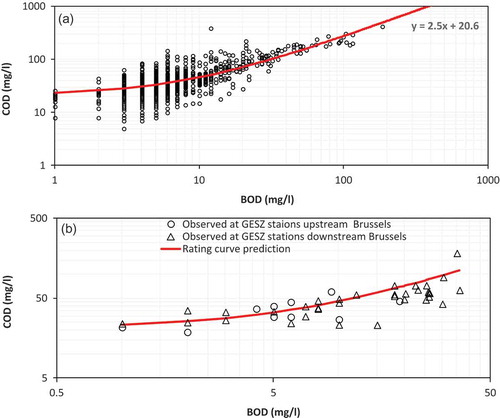
To convert BOD to COD, an analysis was made of the observations at 12 VMM stations upstream from Brussels for the period 1990–2010 (Fig. 4(a)). The results show a typical ratio of 2.5 between COD and BOD (r = 0.83, n = 1222). The derived relationship reproduced BOD and COD pairs observed at GESZ sampling stations upstream (r = 0.54, n = 10) and downstream (r = 0.69, n = 35) from Brussels reasonably well (Fig. 4(b)).

Figure 4. (a) The relation between BOD and COD in the River Zenne upstream of Brussels. (b) Validation of the GESZ measurements against the rating curve.

2.6.4.2 COD fractioning

To fraction the COD into the different state variables used by the RWQM1 formulation, we tested the fractioning proposed by Henze (1992), based on an analysis of influents and effluents of WWTPs. The fractions for the rural catchment runoff were tuned heuristically using the data from the GESZ measurement campaigns at three GESZ stations upstream of Brussels (Z1 to Z3). Similarly, to determine the COD fractions of the WWTP effluents, we used the data from the GESZ measurements of the effluents of two major WWTPs in the Brussels region, Brussels-North and Brussels-South. Finally, we used the GESZ data of influents to these WWTPs to derive COD fractions for WWTP influents. For the CSOs, we had data from only one sampling campaign. Hence, we used the COD fractions of WWTP influents. However, it should be noted that the composition of organic matter in dry weather flow sewage and wet weather sewage can be completely different due to in-sewer transformations (Hvitved-Jacobsen et al. 2002). Table 4 presents the original and adapted fractions.

Table 4. The original and adjusted COD fractions of Henze (1992) for WWTP influents, effluents and for the rural catchment runoff.

	WWTP influent		WWTP effluent
Variable	Original fractions	Modified fractions	Original fractions	Modified fractions	Rural catchment runoff fractions
SS	0.400	0.259	0.067	0.289	0.289
SI	0.025	0.016	0.489	0.378	0.378
XS	0.275	0.477	0.200	0.151	0.133
XI	0.100	0.173	0.178	0.178	0.178
XH	0.198	0.073	0.066	0.004	0.022
XN1	1.25 × 10^−^3	1.25 × 10^−^3	1.11 × 10^−^4	4 × 10^−^5	1.11 × 10^−^5
XN2	1.25 × 10^−^3	1.25 × 10^−^03	1.11 × 10^−^4	4 × 10^−^5	1.11 × 10^−^5
Total	1.00	1.00	1.00	1.00	1.00

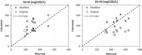
The adapted fractions hold reasonably well for different organic fractions and bio-masses at the considered sampling stations (GESZ stations Z1 to Z3, Fig. 5). Figure 6 presents a comparison between calculated and measured organic fractions and bio-masses at the effluents of the Brussels WWTPs, with default and adjusted fractions (Table 4). Figure 7 shows the same factors at the influents of the Brussels WWTPs corresponding to default and adapted fractioning (Table 4). Figure 7 also includes a CSO measurement carried out during a GESZ sampling campaign. Although only one measurement is available, the figure seems to indicate that the adapted fractioning for WWTP influents can also be used for CSO loadings.

Figure 5. Plot of observed and calculated RWQM1 variables (using Henze’s COD fractioning; Henze 1992) at GESZ stations upstream of Brussels.

Figure 6. Observed and calculated RWQM1 variables (using Henze’s COD fractioning; Henze 1992) of the effluents of the Brussels WWTPs.

Figure 7. Observed and calculated organic fractions for the influent of the Brussels WWTPs. Larger markers are for a CSO event monitored in the GESZ sampling campaign.

Table 5 shows how different RWQM1 components at different input locations were used or approximated. For instance, daily time series of some RWQM1 components were available for the WWTP effluents, while other components were determined using a constant concentration based on the GESZ measurements. Based on the total population living in the command area of a WWTP and on the number of inhabitants connected to the WWTP, the number of unconnected inhabitants could be calculated (Table 5). First, it was assumed that only half of the unconnected inhabitants discharge directly to the water body and other half have alternatives such as septic tanks. Such extra sources were implemented as a constant pollution source discharging at or near their respective WWTPs. Additionally, illicit sewage connection at Brussels was also considered, with an estimate of 30 000 inhabitants-equivalent as in Petrovic et al. (2012).

Table 5. Data sources of the RWQM1 components.

	RWQM1 components
Input Locations	SS	SI	SNH4	SNH3	SNO2	SNO3	SHPO4	SH2PO4	SO2	SCO2	SHCO3	SCO3	SH	SOH	Sca	XH	XN1	XN2	XALG	XCON	XS	XI	XP	XII
Tributaries	a,b	a,b	a	f	a	a	a	f	a	c,e	c,e	c,e	c,e	c,e	c,e	a,b	a,b	a,b	a	f	a,b	a,b	c,e	f
WWTP effluents	d,b	d,b	d	f	d	d	d	f	c,e	c,e	c,e	c,e	c,e	c,e	c,e	d,b	d,b	d,b	f	f	d,b	d,b	c,e	f
Untreated sewage	c,e	c,e	c,e	f	c,e	c,e	c,e	f	c,e	c,e	c,e	c,e	c,e	c,e	c,e	c,e	c,e	c,e	f	f	c,e	c,e	c,e	f
CSO	c,e	c,e	c,e	f	c,e	c,e	c,e	f	c,e	c,e	c,e	c,e	c,e	c,e	c,e	c,e	c,e	c,e	f	f	c,e	c,e	c,e	f
River outlet	c,e	c,e	c,e	f	c,e	c,e	c,e	f	c,e	c,e	c,e	c,e	c,e	c,e	c,e	c,e	c,e	c,e	f	f	c,e	c,e	c,e	f
WWTP	Total population*	Connected population**	Unconnected population	Fraction^#
a: SWAT simulated; b: based on COD fractioning; c: based on GESZ measurements; d: measured time series; e: constant; f: data not available or considered zero concentration.
Unconnected sources
Beersel	70 193	45 825	24 368	0.5
Sint Pieters Leeuw	39 700	28 463	11 231	0.5
Grimbergen	105 000	71 715	33 285	0.5
Zemst Hofstade	12 860	4 392	8 468	0.5
Illicit source, Brussels^†	–	–	30 000	1

*Situation in 2005.

**Situation at the start of the GESZ sampling campaign (September 2009).

^#Only a certain fraction of the total unconnected inhabitants were considered to be discharging directly to the water bodies.

^†Based on the estimate of Petrovic et al. (2012).

Finally, we applied a manual calibration strategy to fine tune the parameters of the integrated water quality model. For this, we used the same stoichiometric parameters and mass fractions of H, O, C, N and P for organic matter, as suggested by Reichert et al. (2001b), which implies that only the kinetic parameters were fine tuned using the GESZ measured dry-weather flow concentrations of various water quality variables. We then validated the integrated model for a long period which also included storm conditions using the (monthly) data for four RWQM1 components (S_O2, S_NH4, S_NO3 and S_HPO4) measured by VMM stations at three locations (Lot, Vilvoorde and Eppegem) during the period 2007–2010.

2.7 Model performance evaluation

Three goodness-of-fit statistics, namely the percentage bias (PBIAS), the ratio of the root mean square error to the standard deviation of the measured data (RSR) and the Nash-Sutcliffe efficiency coefficient (NSE) (Nash and Sutcliffe 1970), were used for model performance evaluation:

(7) $\mathrm{P}\mathrm{B}\mathrm{I}\mathrm{A}\mathrm{S}=\frac{{\sum }_{i=1}^N\left(X_{\mathrm{s}\mathrm{i}\mathrm{m},i}-X_{\mathrm{o}\mathrm{b}\mathrm{s},i}\right)}{{\sum }_{i=1}^N\left(X_{\mathrm{o}\mathrm{b}\mathrm{s},i}\right)}\times 100$(7)

(8) $\mathrm{R}\mathrm{S}\mathrm{R}=\frac{\sqrt{{\sum }_{i=1}^N{\left(X_{\mathrm{s}\mathrm{i}\mathrm{m},i}-X_{\mathrm{o}\mathrm{b}\mathrm{s},i}\right)}^2}}{\sqrt{{\sum }_{i=1}^N{\left(X_{\mathrm{o}\mathrm{b}\mathrm{s},i}-\overline{X_{\mathrm{o}\mathrm{b}\mathrm{s},i}}\right)}^2}}$(8)

(9) $\mathrm{N}\mathrm{S}\mathrm{E}=1-\frac{{\sum }_{i=1}^N{\left(X_{\mathrm{s}\mathrm{i}\mathrm{m},i}-X_{\mathrm{o}\mathrm{b}\mathrm{s},i}\right)}^2}{{\sum }_{i=1}^N{\left(X_{\mathrm{o}\mathrm{b}\mathrm{s},i}-\overline{X_{\mathrm{o}\mathrm{b}\mathrm{s},i}}\right)}^2}$(9)

where X_sim is the simulated quantity, X_obs is the observed quantity, σ_sim is the standard deviation of simulated quantities, σ_obs is the standard deviation of observed quantities and N is the total number of observations.

Based on the range of values of these statistical indicators, we used four performance ratings, Very Good, Good, Satisfactory and Unsatisfactory, to assign qualitative ratings to simulation results, an approach suggested by Moriasi et al. (2007). An average performance rating was then determined by averaging the ratings of the three indicators.

3 Results and discussion

3.1 Streamflow results

The SWAT-simulated streamflow when compared with observed flows at Tubize (Fig. 8(a)) for the calibration (1998/08) and validation (1994/97) periods shows the model’s ability to reproduce the trend of observations. The corresponding goodness-of-fit statistics (Table 6) indicate Very Good and Good model results for the calibration and validation periods, respectively.

Table 6. Goodness-of-fit statistics and final performance rating of different component models of the integrated water quality model.

Variables	Station	Model	Period	Time span	No. of obs.	PBIAS (%)	RSR	NSE	Performance rating^#
Streamflow	Tubize*	SWAT standalone	Calibration	1998–2008	4018	−7.58	0.46	0.79	Very good
			Validation	1994–1997	1461	3.00	0.59	0.65	Good
	Lot	Integrated	Calibration	2007–2008	17544	−11.38	0.57	0.68	Good
			Validation	2009–2010	17503	47.43	0.95	0.11	Unsatisfactory
	Vilvoorde		Calibration	2007–2008	17544	0.3	0.57	0.68	Good
			Validation	2009–2010	17520	−3.38	0.66	0.53	Good
	Eppegem		Calibration	2007–2008	17544	7.94	0.53	0.71	Good
			Validation	2009–2010	17520	21.23	0.69	0.53	Satisfactory
Temperature	U/S Brussels	Standalone	Calibration	1990–2010	626	2.50 × 10^−4	0.40	0.81	Very good
	Lot	Integrated	Validation	2007–2010	47	20.54	0.51	0.74	Good
	Vilvoorde		Validation	2007–2010	72	−3.45	0.43	0.82	Very good
	Eppegem		Validation	2007–2010	75	−3.00	0.29	0.91	Very good
Water quality components
DO	Quenast	SWAT standalone	Calibration	1998–2008	171	−14.78	0.76	0.42	Satisfactory
BOD					118	15.88	1.31	−0.74	Satisfactory
NH4					142	10.87	0.98	0.03	Satisfactory
NO3					141	45.64	2.17	−3.71	Unsatisfactory
DIS-P					141	23.92	1.02	−0.04	Satisfactory
DO	Quenast	SWAT standalone	Validation	1994–1997	36	−18.21	0.99	0.00	Unsatisfactory
BOD					36	33.28	1.56	−1.50	Unsatisfactory
NH4					36	0.60	0.97	0.03	Satisfactory
NO3					36	65.80	3.74	−2.83	Unsatisfactory
DIS-P					36	30.74	1.45	−1.17	Unsatisfactory
SO2	GESZ stations (DWF)	Integrated	Calibration	**	13	−12.34	0.76	0.43	Satisfactory
SS					13	1.49	0.70	0.51	Good
XH					13	−1.56	0.87	0.25	Satisfactory
XN1					7	−26.69	0.87	0.14	Satisfactory
SNH4					13	−12.24	0.55	0.69	Good
SNO3					13	9.96	0.77	0.41	Satisfactory
SHPO4					13	−10.98	0.42	0.82	Very good
pH					13	−1.79	2.29	−4.22	Satisfactory
EC25degC					13	−7.96	0.78	0.40	Satisfactory
SO2	Lot	Integrated	Validation	2007–2010	45	11.53	0.54	0.71	Good
SNH4					45	−30.19	1.05	−0.10	Unsatisfactory
SNO3					45	37.04	2.44	−4.96	Unsatisfactory
SHPO4					44	−6.79	0.69	0.52	Good
SO2	Vilvoorde	Integrated	Validation	2007–2010	66	−2.53	0.96	0.08	Satisfactory
SNH4					54	−23.58	0.85	0.28	Satisfactory
SNO3					53	57.81	1.28	−0.63	Unsatisfactory
SHPO4					54	−6.84	0.71	0.50	Satisfactory
SO2	Eppegem	Integrated	Validation	2007–2010	70	41.96	0.98	0.04	Unsatisfactory
SNH4					54	−29.20	1.11	−0.22	Satisfactory
SNO3					53	38.44	1.32	−0.75	Unsatisfactory
SHPO4					54	−18.36	0.94	0.11	Satisfactory
Performance rating	PBIAS (%) Streamflow	PBIAS (%) Water quality	RSR	NSE	Colour scheme
Very good	<±10	<±15	0 to 0.5	0.75 to 1
Good	±10 to ±15	±15 to ±30	0.5 to 0.6	0.65 to 0.75
Satisfactory	±15 to ±25	±30 to ±55	0.6 to 0.7	0.5 to 0.65
Unsatisfactory	>±25	>±55	>0.7	<0.5

* Tubize is located approximately 4 km downstream of Quenast.

** Five GESZ sampling campaigns were conducted from September 2009 to October 2010.

^# Based on Moriasi et al. (2007).

Figure 8. Observed and simulated streamflows at (a) Tubize and (b) Vilvoorde during calibration and validation periods.

Figure 8(b) shows the results of the SWAT-SWMM integrated model for streamflow at Vilvoorde. The SWAT-SWMM integrated model reproduces the streamflow with Good accuracy (Table 6) for both calibration (2007/08) and validation (2009/10) periods. The accuracy of the integrated model at Lot (upstream of Brussels) is Good and Unsatisfactory for the calibration and validation periods, respectively (Table 6). Similarly, the goodness-of-fit indicated quality of model results of Good and Satisfactory for the calibration and validation periods, respectively, at Eppegem (downstream of Brussels).

Various factors (e.g. differences in rainfall patterns) could produce slight underperformance of model results for the validation period as compared with the calibration period. However, the observed low flows in the validation period are systematically higher than in the calibration period, while the simulated low flows are comparable (Fig. 8(b)). Hence, it is evident that the difference is related to the quality of observed streamflows.

For clarity, the optimized streamflow-related SWAT and SWMM parameters are not presented here, and readers are referred to Leta et al. (2012).

3.2 Temperature results

Table 7 shows the optimized parameters of the temperature model. Similarly, Figure 9 presents the integrated stream water temperature model results at Vilvoorde. The model reproduces the trend of observation very well, as also evident in the goodness-of-fit statistics (Table 6), which point to Very Good model results. For the integrated temperature model, except at Lot (where overestimation of about 20% was observed), the model results are Very Good (Table 6).

Table 7. Optimized parameters of different component models of the integrated water quality model.

Parameters	Description	Unit	Range/Default values	Calibrated values
(A) SWAT model (QUAL2E parameters)*
Kinetic parameters:
K1	De-oxygenation coefficient	1/d	0.02–3.4	1.3
K2	Re-aeration coefficient	1/d	0–100	4
K3	BOD settling rate	1/d	−0.36–0.36	0.36
K4	Sediment oxygen demand rate	mgO2/m^2 d	variable	1
σ1	Algal settling rate	1/d	0.5–6	0.1
σ2	Benthic source rate for P	mgP/m^2 d	variable	0.01
σ3	Benthic source rate for N	mgNH4/m^2 d	variable	0.2
σ4	N settling rate	1/d	0.001–0.1	0.1
σ5	P settling rate	1/d	0.001–0.1	0.1
β1	Ammonia oxidation rate	1/d	0.1–1	0.1
β2	Nitrite oxidation rate	1/d	0.2–2	0.1
β3	N hydrolysis rate	1/d	0.02–0.4	0.3
β4	P hydrolysis rate	1/d	0.01–0.7	0.55
μmax	Maximum algal growth	1/d	1–3	2.2
ρ	Algal respiration rate	1/d	0.05–0.5	0.2
Stoichiometric parameters*
α3	Oxygen production rate per unit of algal growth	–	1.4–1.8	1.6
α4	Oxygen uptake per unit of algal respiration	–	1.6–2.3	2
FNH4	Ammonia preference factor	–	0–1	0.5
(B) Temperature model
μ	Minimum stream temperature	°C	–	1.98
α	Estimated maximum stream temperature	°C	–	30.21
γ	Steepest slope (inflection point) of the Ts function	–	–	0.1
β	Air temperature at this inflection point	°C	–	19.05
Lag	Lag period	d	–	2
(C) Integrated water quality model (RWQM1)
Kinetic parameters**
kgro_H_aer_To	Maximum aerobic specific growth rate of heterotrophs	1/d	2	3.5
kgro_H_anox_To	Maximum anoxic specific growth rate of heterotrophs	1/d	1.6	2
khyd_To	Hydrolysis rate constant	1/d	3	0.2
kres_H_aer_To	Maximum aerobic specific respiration rate of heterotrophs	1/d	0.2	4
kres_H_anox_To	Maximum anoxic specific respiration rate of heterotrophs	1/d	0.1	1.6
kres_N1_To	Maximum specific respiration rate of 1st stage nitrifiers	1/d	0.05	3
KNO3_H_anox	Saturation coefficient for anoxic growth of heterotrophs on nitrate	mgN/L	0.5	0.1
KNO2_H_anox	Saturation coefficient for anoxic growth of heterotrophs on nitrite	mgN/L	0.2	0.1
KO2_H_aer	Saturation/inhibition coefficient for aerobic endogenous respiration of heterotrophs	mgSO2/L	0.2	1
KS_H_anox	Saturation coefficient for anoxic growth of heterotrophs on dissolved substrate	mgXH/L	2	0.7
kreaer_To	Re-aeration coefficient	1/d	-	0.2

Stoichiometric parameters: same as specified in Reichert et al. (2001b).

Mass fraction of elements on organic compounds: same as specified in Reichert et al. (2001b).

* Range of values taken from Brown and Barnwell (1987).

** Only the parameters differing from their default values as specified in Reichert et al. (2001b) are presented.

Figure 9. Observed and simulated stream water temperature at Vilvoorde.

3.3 Water quality results

3.3.1 SWAT results

Table 7 shows the optimized QUAL2E parameters (kinetic and stoichiometric). Similarly, Figure 10(a)–(d) presents simulated and observed DO, BOD, NO₃ and DIS-P, respectively, at Quenast for the calibration and validation periods. The corresponding goodness-of-fit statistics along with a final performance rating are presented in Table 6. In general, all the simulated components follow the trend of observations. However, the lack of data in extreme conditions is well reflected in the NO₃ plot, where the concentration crossed the 30 mg/L mark, while measurements of up to 10 mg/L were recorded. As there is extensive use of fertilizers in the agriculture-dominated upstream sub-catchments, the simulated levels of NO₃ would be expected, but we do not have observations to verify this.

Figure 10. Observed and simulated (a) DO, (b) BOD, (c) NO₃, and (d) dis-P at Quenast during calibration and validation periods.

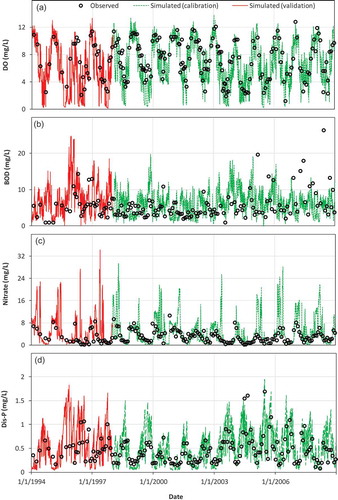
In terms of qualitative ratings, all components except NO₃ are simulated with Satisfactory accuracy in the calibration period. For NO₃, the model results are Unsatisfactory. On average, the model overestimates the NO₃ concentrations by 47%. For the validation period, except for NH₄, for which the performance rating is Satisfactory, the model results are Unsatisfactory. However, it should be noted that a higher number of samples (>100) was used to calculate the statistics for the calibration period, while only 36 observations were available for the validation period (Table 6).

3.3.2 Integrated model results

3.3.2.1 Dry weather flow (DWF) simulation

Table 7 shows the optimized (kinetic) parameters of the integrated water quality model. Similarly, Figure 11(a)–(g) shows simulated and observed (represented by a boxplot constructed using the observations made in five GESZ sampling campaigns) S_S, S_O2, S_NH4, S_NO3, S_HPO4 and X_H, respectively, at GESZ sampling stations.

Figure 11a. Observed and simulated (a) S_S, (b) S_O2, (c) S_NH4, (d) S_NO3, (e) S_HPO4, (f) X_H, (g) X_H (represented as pH) and EC₂₅ at 13 GESZ sampling stations during DWF conditions.

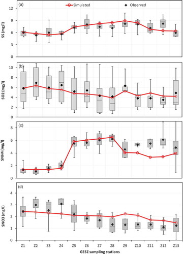
Figure 11b. (Continued).

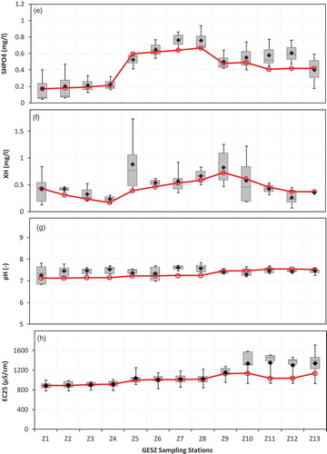
In the river reach between the sampling stations Z1 and Z4, there are only small WWTPs, so pollution to the river is fairly limited. As such, the level of S_O2 seems to be relatively high and remains fairly stable in the reach (Fig. 11(b)). With relatively high S_O2 levels, X_H and nitrifiers (X_N1 and X_N2) are mainly responsible for the slight decrease of the S_S levels in the reach (Fig. 11(a)). The presence of few or no pollution sources in the reach is also reflected in the rather stable concentrations of S_NH4 and S_HPO4 (Fig. 11(c) and (e)). At station Z5, there is a marked increase in S_S, S_NH4, S_HPO4 and X_H. This could be attributed mainly to the effluents from the Brussels-South WWTP (360 000 IE) because there are suggestions (e.g. Garnier et al. 2013) that the WWTP is not functioning well and untreated effluent is often discharged into the river. Moreover, as station Z5 lies just downstream of the confluence of the Zenne with a tributary, the Zuunbeek, which the measurements made during the GESZ sampling campaigns showed to be highly contaminated, the marked increase could also be due to this tributary. After station Z5, the concentrations of S_S, S_NH4, S_HPO4 and X_H tend to increase due to unknown illicit sewage disposal (Table 5). In contrast to the Brussels-South WWTP, the Brussels-North WWTP, which is situated just before the GESZ station Z9, tends to increase the S_O2 concentrations while decreasing S_NH4 and S_HPO4 concentrations, exhibiting a clear dilution effect. The increased concentrations of S_S and X_H would mean that more “grazing” of S_S by X_H is expected, as plenty of food for X_H is available. Overall, the effluents of the Brussels-North WWTP tend to improve the ecological status of the river. After station Z9, the only major polluter is the effluent of the Grimbergen WWTP, which treats about 100 000 IE and is situated just upstream of station Z10, and hence shows no significant change in the concentration of major components. The return flow from the canal discharges just before station Z10, and tends to have a positive impact, mainly by dilution, on the ecological status of the river, which is reflected in increased S_O2 concentrations and decreased concentrations of other components including S_S. As the river experiences a diurnal tide (normally in the reaches downstream of station Z11), larger variations in the concentrations of the components (as indicated by large error bars of the boxplots) are expected and duly observed. The situation is evident at the GESZ station Z13, the most downstream station. From the observed concentrations of S_NH4 and S_HPO4, it can be deduced that some unknown pollution sources exist in the reaches between GESZ stations Z11 and Z12, which are obviously not considered in the model.

From the results, it can be stated that the integrated model was able to simulate the trend of observations of all the RWQM1 components. In terms of qualitative ratings, the integrated model was able to simulate S_HPO4 with Very Good accuracy, two components – S_S and S_NO3, with Good accuracy, and only Satisfactory accuracy was obtained for the remaining components.

From a management point of view, the ecological status of the river during DWF is rather poor. For example, the EU Freshwater Fish Directive (78/656/EEC) recommends a minimum S_O2 level of 6 mg/L (for “Salmonid” waters), which was the case for GESZ stations Z1–Z4 (upstream of Brussels). It was observed that even after the construction of the two largest WWTPs in Brussels, the S_O2 concentrations remained lower than the mandatory level (6 mg/L). The Brussels-North WWTP effluents had a positive impact but the reaches downstream (Z10–Z13) remained low in S_O2 concentration. In terms of S_NH4 levels, the River Zenne’s ecological status is poor, as S_NH4 levels of more than 1 mg/L (for “Salmonid” waters) were observed in almost all reaches of river. Hence, the Zenne requires a lot of work to acquire the desired ecological status.

3.3.2.2 Long-term simulation

For long-term simulation, due to lack of data for all RWQM1 components, the model is validated against the four components (S_O2, S_NH4, S_NO3 and S_HPO4) at Lot, Vilvoorde and Eppegem (Figs. 12–14).

Figure 12. Observed and simulated (hourly) (a) S_O2, (b) S_NH4, (c) S_NO3 and (d) S_HPO4 at Lot.

Figure 13. Observed and simulated (hourly) (a) S_O2, (b) S_NH4, (c) S_NO3 and (d) S_HPO4 at Vilvoorde.

Figure 14. Observed and simulated (hourly) (a) S_O2, (b) S_NH4, (c) S_NO3 and (d) S_HPO4 at Eppegem.

While the integrated model tends to overestimate the S_O2 concentrations at Lot (Fig. 12(a)) during summer, as also indicated by a rather high PBIAS value of about 12%, the model was able to capture the S_O2 concentrations during winter reasonably well. As such, the overall simulation was of Good quality (Table 6). However, the S_NH4 concentrations are hugely underestimated (Fig. 12(b)), as reflected in the goodness-of-fit statistics, which indicated Unsatisfactory quality of model results. It should be noted that the model simulated the S_NH4 concentrations very well under DWF conditions at the GESZ stations Z1–Z4 (upstream of Brussels) and that the Lot station is in between GESZ stations Z2 and Z3; thus, the underestimation could not be related to the (calibrated) parameter values, rather it could be related to the presence of illicit pollution sources in the reach, which were obviously not considered in the model. The simulated concentrations of S_NO3 are still overestimated by more than 37%, as observed in SWAT simulations at Quenast. The reach between Quenast and Lot is too short to undergo significant conversion in terms of the S_NO3 concentrations. This serious overestimation was also reflected in the overall quality of the S_NO3 simulation results, which, according to goodness-of-fit statistics, was Unsatisfactory (Table 6). As for S_HPO4, the simulation results improved, leading to Good quality, as apparent in the graphical plot (Fig. 12(d)), where simulated concentrations follow the trend of observations.

At Vilvoorde, the model reproduces the trend of the S_O2 concentrations (Fig. 13(a)) fairly well, as evident in the final performance rating, which is Satisfactory. Note that the station is located just after the Brussels-North WWTP and, while building up the model, we imposed a constant S_O2 concentration (Table 5) throughout the year due to lack of measured time series of S_O2 in the WWTP effluent. While significant variations under wet conditions are expected, under DWF conditions, the input variations are damped due to the long residence times in the Brussels-North WWTP (order of magnitude ≈ 1 week). In fact, the manager of the WWTP is not legally obliged to measure the S_O2 concentrations in the WWTP effluents. The mismatch of the S_O2 concentrations for the winter half-year might be related to this. The Brussels-North WWTP could have been discharging effluents that have seasonal variations in S_O2. During the winter half-year, the S_O2 concentrations may be higher than the imposed concentration (of 6.5 mg/L; estimated based on GESZ measurements). Consequently, the underestimation of S_O2 concentration is reflected in a rather high value of PBIAS (≈24%). The plot also shows evidence of the effect of CSO overflows on the S_O2 concentration, in frequent drops during wet conditions. While the S_O2 levels fell, the concentrations remained generally above 2.5 mg/L throughout, even though the CSO events released highly concentrated, readily biodegradable organic matter. The Vilvoorde station is located (too) close to the CSO outlets, such that biodegradation processes did not have enough time to significantly deplete S_O2 levels. As observed in the case of Lot, the model underestimates the S_NH4 concentrations (Fig. 13(b)) and overestimates the S_NO3 concentrations (Fig. 13(c)). A slightly better result for S_HPO4 (Fig. 13(d)) is observed, as reflected in the overall quality of model results being Satisfactory (Table 6).

At Eppegem, the effect of CSO overflows on S_O2 depletion can be observed more clearly. The S_O2 concentrations (Fig. 14(a)) even reached 0.5 mg/L on some occasions. While the simulated S_O2 tends to follow the observations, the qualitative rating was calculated to be Unsatisfactory (Table 6). On average, the S_O2 concentrations were overestimated by 42%. For S_NH44 (Fig. 14(b)) and S_NO3 (Fig. 14(c)), the same trend of underestimation and overestimation, respectively, as for the Lot and Vilvoorde stations is observed. The model results for S_HPO4 (Fig. 14(d)) show a fair match between observed and simulated concentrations, and the qualitative rating is Satisfactory (Table 6). However, on average, the model underestimated the S_HPO4 concentrations. While S_O2 concentrations are overestimated, S_NH4 and S_HPO4 concentrations are underestimated; this could indicate the presence of possible unknown sources in the reach. Or it could be because of improper boundary conditions (SWAT simulated) at canal inlet points, as the station is located just downstream of the return flow from the canal to the river.

4 Conclusions

We have successfully used the OpenMI standard in integrating four models (SWAT, SWMM, temperature and water quality) and used this integrated model to simulate various water quality components of the River Zenne in Belgium. The water quality model was based on recently developed IWA RWQM1 principles. As SWAT employs the QUAL2E formulation for its water quality conversion processes, we also addressed the reconciliation issues between QUAL2E–RWQM1 state variables. For this, we adapted COD fractions as calculated by Henze (1992).

Although the RWQM1 formulation is founded on state-of-the-art of water quality modelling principles, it is rather complex, especially for calibration and validation tasks. Consequently, we could not calibrate or validate the model properly. This is because: (a) observed data were only available for very few components of the formulation, leading us to impose constant input concentrations (based on the GESZ sampling campaigns); (b) very few studies have been reported where the formulation is used for biochemical conversion processes in rivers and, consequently, very little is known about the parameters of the formulation; thus, calibration of the integrated model became difficult; and (c) we could not validate all the RWQM1 components because of the problems highlighted earlier.

However, despite difficulties in model build-up, calibration and validation, the integrated water quality model simulated various water quality components with a wide range of accuracy (Unsatisfactory to Very Good). In terms of ecological status, the river is far from the goals set by the EU Water Framework Directive, under both dry weather and storm conditions, in almost all reaches of the river.

Acknowledgements

We would like to thank several agencies (RMI, VMM, DGVH and DGARNE) for providing the data. We are thankful to all our colleagues from the GESZ project for providing the data and valuable suggestions, especially Professor Natacha Brion (VUB-AHCH), Professor Ann van Griensven (VUB-HYDR) and Dr Burno de Fraine (VUB-DINF).

Disclosure statement

No potential conflict of interest was reported by the authors.

Additional information

Funding

We would like to thank INNOVIRIS – (Brussels Institute for Research and Innovation) for supporting the GESZ research project.

References

- Argent, R.M., et al., 2006. Comparing modelling frameworks – A workshop approach. Environmental Modelling & Software, 21 (7), 895–910. doi:10.1016/j.envsoft.2005.05.004
- Arnold, J.G., et al., 1998. Large-area hydrologic modelling and assessment: part I. Model development. Journal of the American Water Resources Association, 34 (1), 73–89. doi:10.1111/j.1752-1688.1998.tb05961.x
- Arnold, J.G., et al., 2011. Soil and Water Assessment Tool input/output file documentation, version 2009. Texas: Agrilife Blackland Research Center.
- Betrie, G.D., et al., 2011. Linking SWAT and SOBEK using open modelling interface (OpenMI) for sediment transport simulation in the Blue Nile river basin. Transactions of the American Society of Agricultural and Biological Engineers, 54 (5), 1749–1757.
- Borchardt, D. and Reichert, P., 2001. River water quality model no. 1 (RWQM1): case study. I. Compartmentalisation approach applied to oxygen balances in the River Lahn (Germany). Water Science & Technology, 43 (5), 41–49.
- Broekhuizen, N., et al., 2012. Modification, calibration and verification of the IWA river water quality model to simulate a pilot-scale high rate algal pond. Water Research, 46 (9), 2911–2926. doi:10.1016/j.watres.2012.03.011
- Brown, L. and Barnwell, T., 1985. Computer program documentation for the enhanced stream water quality model QUAL2E. Athens: US EPA, Environmental Research Laboratory, Georgia.
- Brown, L. and Barnwell, T., 1987. The enhanced stream water quality models QUAL2E and QUAL2E-UNCAS: Documentation and user manual. Athens: US EPA, Environmental Research Laboratory, Georgia.
- Bulatewicz, T., et al., 2010. Accessible integration of agriculture, groundwater, and economic models using the open modelling interface (OpenMI): methodology and initial results. Hydrology and Earth Systems Sciences, 14 (3), 521–534. doi:10.5194/hess-14-521-2010
- Bulatewicz, T., et al., 2013. The simple script wrapper for OpenMI: Enabling interdisciplinary modelling studies. Environmental Modelling & Software, 39 (0), 283–294. doi:10.1016/j.envsoft.2012.07.006
- Candela, A., et al., 2012. Receiving water body quality assessment: an integrated mathematical approach applied to an Italian case study. Journal of Hydroinformatics, 14 (1), 30–47. doi:10.2166/hydro.2011.099
- Council Directive. 2000. Establishing a framework for community action in the field of water policy. Official Journal of the European Communities. L327: 1-72.
- Demuynck, C., et al., 1997. Evaluation of pollutant reduction scenarios in a river basin: application of long term water quality simulations. Water Science & Technology, 35 (9), 65–75. doi:10.1016/S0273-1223(97)00185-6
- Garnier, J., et al., 2013. Modelling historical changes in nutrient delivery and water quality of the Zenne River (1790s–2010): the role of land use, waterscape and urban wastewater management. Journal of Marine Systems, 128, 62–76. doi:10.1016/j.jmarsys.2012.04.001
- Grant, P.J., 1977. Water temperatures of the Ngaruroro River at three stations. Journal of Hydrology (New Zealand), 16 (2), 148–157.
- Gregersen, J.B., Gijsbers, P.J.A., and Westen, S.J.P., 2007. OpenMI: Open modelling interface. Journal of Hydroinformatics, 9 (3), 175–191. doi:10.2166/hydro.2007.023
- Hayashi, M., 2004. Temperature-electrical conductivity relation of water for environmental monitoring and geophysical data inversion. Environmental Monitoring and Assessment, 96 (1–3), 119–128. doi:10.1023/B:EMAS.0000031719.83065.68
- Henze, M., 1992. Characterization of wastewater from modelling of activated sludge processes. Water Science & Technology, 25 (6), 1–25.
- Henze, M., et al., 2000. Activated sludge models ASM1, ASM2, ASM2d and ASM3. London: IWA publishing.
- Hvitved-Jacobsen, T., Vollertsen, J., and Matos, J.S., 2002. The sewer as a bioreactor - a dry weather approach. Water Science & Technology, 45 (3), 11–24.
- Krebs, P., et al., 1999. First flush of dissolved components. Water Science & Technology, 39 (9), 55–62. doi:10.1016/S0273-1223(99)00216-4
- Lai, C., 1987. Numerical modelling of unsteady open-channel flow. In: B.C. Yen, ed. Advances in Hydroscience. New York: Academic Press, 161–333.
- Laniak, G.F., et al., 2013. Integrated environmental modelling: a vision and roadmap for the future. Environmental Modelling & Software, 39 (0), 3–23. doi:10.1016/j.envsoft.2012.09.006
- Leta, O.T., et al., 2011. Accessible linking of hydrological and hydraulic models through OpenMI for integrated river basin management. Water 2011: Integrated water resources management in tropical and subtropical drylands. Mekelle: KU Leuven and Mekelle University.
- Leta, O.T., et al., 2012. OpenMI Based Flow and Water Quality Modelling of the River Zenne. In: Societe Hydrotechnique de France, ed. 2nd International conference - SimHydro 2012. France: Nice-Sophia Antipolis.
- Leta, O.T. 2014. Integrated water quality modelling of the river Zenne (Belgium) using OpenMI. In: P. Gourbesville, et al., eds. Advances in Hydroinformatics – SIMHYDRO 2012 – New frontiers of simulation. Singapore: Springer Singapore, 259–274.
- Marijns, F. and Bauwens, W., 1997. The application of activated sludge model no.1 to a river environment. Water Science & Technology, 36 (5), 201–208. doi:10.1016/S0273-1223(97)00475-7
- Martín, C., et al., 2006. Dynamic simulation of the water quality in rivers based on the IWA RWQM1. Application of the new simulator CalHidra 2.0 to the Tajo River. Water Science & Technology, 54 (11–12), 75–83. doi:10.2166/wst.2006.741
- Masch, F.D., 1971. Simulation of water quality in streams and canals: Theory and description of the QUAL-I mathematical modelling system. Austin: Texas Water Development Board.
- Masliev, I., Somlyody, L., and Koncsos, L., 1995. On reconciliation of traditional water quality models and activated sludge models. Laxenburg: Internation Institute for Applied System Analysis, Austria.
- Mohseni, O., Stefan, H.G., and Erickson, T.R., 1998. A nonlinear regression model for weekly stream temperatures. Water Resources Research, 34 (10), 2685–2692. doi:10.1029/98WR01877
- Moore, R.V. and Tindall, C.I., 2005. An overview of the open modelling interface and environment (the OpenMI). Environmental Science & Policy, 8 (3), 279–286. doi:10.1016/j.envsci.2005.03.009
- Moriasi, D.N., et al., 2007. Model evaluation guidelines for systematic quantification of accuracy in watershed simulations. Transactions of the ASABE, 50 (3), 885–900. doi:10.13031/2013.23153
- Nash, J.E. and Sutcliffe, J.V., 1970. River flow forecasting through conceptual models part I - A discussion of principles. Journal of Hydrology, 10 (3), 282–290. doi:10.1016/0022-1694(70)90255-6
- OGC, 2016. Open Geospatial Consortium [online]. Available from: http://www.opengeospatial.org/standards/openmi [ Accessed 25 Jul 2016].
- OpenMI, 2009. OpenMI Life Project Website [online]. Open Modelling Interface. Available from: http://www.openmi.org/ [ Accessed 1 Sep 2012].
- Parker, P., et al., 2002. Progress in integrated assessment and modelling. Environmental Modelling & Software, 17 (3), 209–217. doi:10.1016/S1364-8152(01)00059-7
- Peng, J., 1994. Hydraulic residence time of CSTRs under unsteady‐state condition. Journal of Environmental Engineering, 120 (6), 1446–1458. doi:10.1061/(ASCE)0733-9372(1994)120:6(1446)
- Petrovic, D., et al., 2012. Effect of intense rainfall event on metallic and particulate pollutant fluxes in a small urban watercourse. In: Prodanovic, D and Plavsic, J, eds. 9th International Conference on Urban Drainage Modelling. Belgrade: University of Belgrade.
- Reichert, P., 2001. River water quality model no. 1 (RWQM1): case study II. Oxygen and nitrogen conversion processes in the River Glatt (Switzerland). Water Science & Technology, 43 (5), 51–60.
- Reichert, P., et al., 2001a. River water quality model no.1. London: IWA Publishing.
- Reichert, P., et al., 2001b. River water quality model no. 1 (RWQM1): II. Biochemical process equations. Water Science & Technology, 43 (5), 11–30.
- Roesner, L.A.P.R.G. and Evenson, D.E., 1981. Computer program documentation for stream quality model (QUAL-II). Athens: Environmental Research Laboratory, Georgia.
- Rossman, L.A., 2009. Storm Water Management Model user’s manual. Version 5.0. Cincinnati: US EPA, Water Supply and Water Resources Division, National Risk Management Research Laboratory.
- Shanahan, P., et al., 1998. River water quality modelling: II. Problems of the art. Water Science & Technology, 38 (11), 245–252. doi:10.1016/S0273-1223(98)00661-1
- Shrestha, N.K., et al., 2012b. Integrated modelling of river Zenne using OpenMI. In: R. Hinkelmann, et al., eds. 10th International Conference on Hydroinformatics. Hamburg: TuTech Innovation.
- Shrestha, N.K., et al., 2013. OpenMI-based integrated sediment transport modelling of the river Zenne, Belgium. Environmental Modelling & Software, 47 (0), 193–206. doi:10.1016/j.envsoft.2013.05.004
- Shrestha, N.K., et al., 2014. Modelling Escherichia coli dynamics in the river Zenne (Belgium) using an OpenMI. Journal of Hydroinformatics, 16 (2), 354–373. doi:10.2166/hydro.2013.171
- Shrestha, N.K., De Fraine, B., and Bauwens, W., 2012a. SWMM has become OpenMI compliant. In: Prodanovic, D. and Plavsic, J., eds. 9th International Conference on Urban Drainage Modelling. Belgrade: University of Belgrade.
- Somlyody, L., 1982. Water-quality modelling: a comparison of transport-oriented and ecology-oriented approaches. Ecological Modelling, 17, 183–207. doi:10.1016/0304-3800(82)90031-X
- Somlyody, L. and van Straten, G., 1986. Modelling and managing shallow lake eutrophication - with application to Lake Balaton. Berlin: Springer-Verlag.
- Stefan, H.G. and Preud’homme, E.B., 1993. Stream temperature estimation from air temperature. Water Resources Bulletin, 29 (1), 27–45. doi:10.1111/j.1752-1688.1993.tb01502.x
- Streeter, H.W. and Phelps, E.B., 1925. A Study of the pollution and natural purification of the Ohio river. Washington, DC: US Public Health Service.
- van Griensven, A., 2002. Developments towards integrated water quality modelling for river basins. Thesis (PhD). Brussels: Department of Hydrology and Hydraulic Engineering. Vrije Universiteit Brussel (VUB).
- van Griensven, A. and Bauwens, W., 2002. Comparison of process descriptions for river water quality in an integrated modelling context. In: Fifth International Conference on Hydroinformatics. Cardiff: IWA Publishing; p. 439–444.
- Vanrolleghem, P., et al., 2001. River water quality model no. 1 (RWQM1): III. Biochemical submodel selection. Water Science & Technology, 43 (5), 31–40.
- Verbanck, M., 1995. Transferts de la charge particulaire dans l’égout principal de la ville de Bruxelles. Thesis (PhD). Brussels: Department of Water Pollution Control. Université Libre de Bruxelles (ULB).
- Watanabe, M., Harleman, D.R.F., and Vasiliev, O.F., 1983. Two- and three-dimensional mathematical models for lakes and reservoirs. In: G.T. Orlob, ed. Wiley-IIASA international series on applied systems analysis. Chichester, UK: Wiley, 274–336.