Upward infiltration–evaporation method to estimate soil hydraulic properties

ABSTRACT

Determination of saturated hydraulic conductivity, K_s, and the van Genuchten water retention curve θ(h) parameters is crucial in evaluating unsaturated soil water flow. The aim of this work is to present a method to estimate K_s, α and n from numerical analysis of an upward infiltration process at saturation (Cap0), with (Cap0 + h) and without (Cap0) an overpressure step (h) at the end of the wetting phase, followed by an evaporation process (Evap). The HYDRUS model as well as a brute-force search method were used for theoretical loam soil parameter estimation. The uniqueness and the accuracy of solutions from the response surfaces, K_s–n, α–n and K_s–α, were evaluated for different scenarios. Numerical experiments showed that only the Cap0 + Evap and Cap0 + h + Evap scenarios were univocally able to estimate the hydraulic properties. The method gave reliable results in sand, loam and clay-loam soils.

KEYWORDS:

• soil hydraulic properties
• inverse methods
• HYDRUS

Editor R. Woods Associate editor N. Verhoest

1 Introduction

Determination of soil hydraulic properties is of paramount importance in many scientific fields such as agronomy, hydrology and environmental science. Water flow into soil, which depends on the soil’s ability to transmit water through the porous medium, is a function of the pore-size distribution, the tortuosity, and the shape and degree of interconnection of the water-conducting pores (Dane and Hopmans 2002). This process is defined by two main characteristic functions: the hydraulic conductivity, K(h), and the water retention curve, θ(h) (Dane and Hopmans 2002).

The water retention curve is defined as the relationship between the soil volumetric water content (θ) (m³ m⁻³) and the matric potential h (kPa); the shape of this function depends on the soil structure and the particle size distribution. The reference laboratory method employed to determine θ(h) is the pressure extractor (Klute 1986). Tempe cells are commonly used for applying pressure heads corresponding to suctions up to −100 kPa. For higher matric suctions (typically −1500 kPa) more robust pressure cells are needed (Wand and Benson 2004). However, this method is time consuming and is often limited to a relatively narrow range of matric potentials (Simunek et al. 1998a). The K is a measure of the soil’s ability to transmit water when subjected to a hydraulic head gradient; this parameter depends on the soil water content, the pressure head and the flux across the boundary of a soil compartment (Dane and Hopmans 2002). When the porous medium is saturated, K is known as the saturated hydraulic conductivity, K_s (Reynolds 2002). Laboratory determination of K_s is best accomplished using undisturbed soil cores, although repacked cores are used occasionally. Among the different methods used to measure K_s, the constant head method is considered to be a relatively simple, fast and accurate standard procedure (Reynolds 2002). Otherwise, the hydraulic properties can be estimated under laboratory conditions by the evaporation method (Wendroth et al. 1993). Although this method, which needs relatively large soil cores (110 mm internal diameter by 80 mm height), allows simultaneous estimations of θ(h) and K(h), several limitations have been described: (i) it requires using tensiometers for which only a range of tensiometric measurements are possible; (ii) uncertainties in the positions of the tensiometers in the sample; (iii) difficulties in working with undisturbed soil cores (Arya 2002); and (iv) incompatibility with soil cracking during evaporation processes. For K(h) estimation during an infiltration process under constant head, the Green-Ampt approach (Green and Ampt 1911) has been applied successfully (Mohammadzadeh-Habili and Heidarpour 2011).

As an alternative, K_s and θ(h) can be estimated by inverse numerical analysis of the transient water flow using the HYDRUS model, either for a soil wetting (Russo et al. 1991, Simunek and van Genuchten 1996, 1997, Simunek et al. 2001, Young et al. 2002, Rashid et al. 2015, Moret-Fernández et al. 2016) or for an evaporation (Simunek et al. 1998a) process. The main improvement of these optimization procedures is that they allow simultaneous estimation of θ(h) and K(h) (Simunek and van Genuchten 1996). For laboratory conditions, Simunek et al. (1998a) employed the evaporation method to estimate soil hydraulic properties from simultaneous numerical analysis of measured soil water evaporation and soil pressure heads recorded at different depths. The objective function for the parameter estimation analysis was defined in terms of the final total water volume in the core and pressure head readings by one or several tensiometers. The numerically generated data showed that the optimization method was more sensitive to the shape factor (n) and saturated water content (θ_s) than to residual water content (θ_r). The optimized hydraulic parameters corresponded closely with those obtained using the Wind (1968) evaporation method (Simunek et al. 1998a). Young et al. (2002), using pressure head data measured with tensiometers installed in a soil column of 20 cm height and upward water flow at negative pressure heads, calculated the soil hydraulic parameters from the best minimization of the objective function. In other work, Mboh (2011) estimated soil hydraulic parameters in sand by means of water content dynamics measured using the TDR technique under a falling infiltration process. More recently, Moret-Fernández et al. (2016), using a tension sorptivimeter device, estimated soil hydraulic properties from inverse analysis of a multiple tension upward infiltration curve measured on a 5-cm height soil column, without employing tensiometers or soil moisture sensors. The theoretical analysis demonstrated that K_s and θ(h) could be simultaneously estimated if high negative tensions were applied. Similar results were found if medium negative tension plus an overpressure step to calculate K_s by Darcy’s law were applied. The validation of this method on actual sieved soils demonstrated that this technique could be satisfactorily used to estimate, by numerical inverse analysis, soil hydraulic properties. However, as reported by Simunek et al. (1998a) and Moret-Fernández et al. (2016), extrapolation of estimated θ(h) data beyond the range of measured tension is associated with a high level of uncertainty.

The objective of this work is to present a new and easy to perform laboratory method to estimate soil hydraulic parameters by means of inverse analysis of a soil upward infiltration process at saturation plus an overpressure step followed by an evaporation process measured on a 5-cm height soil column, without employing tensiometers and/or soil moisture sensors. The method was tested on theoretical loam soil data generated by the HYDRUS 2D package. The feasibility of this new method under laboratory conditions was tested on sand, and on 2 mm sieved loam and clay-loam soils.

2 Material and methods

2.1 Theory

2.1.1 Water flow in one dimension

Assuming an insignificant role for the air phase in the liquid flow process, the governing equation for one-dimensional flow in a variably saturated rigid porous medium is given by the Richards equation:

(1)

where θ is the volumetric soil water content [L³ L⁻³], t is time [T], z is a vertical coordinate [L] positive upward, h is the soil-water pressure head [L] and K(h) is the unsaturated hydraulic conductivity [L T⁻¹].

For the upward infiltration process, a uniform water content profile corresponding to an air-dried soil is used as the initial condition:

(2)

The boundary conditions (BC) for the upward infiltration processes are either a constant (Cap0, h = 0) or a variable (Cap0 + h) pressure head at the bottom of the soil sample (see Table 1 for details about pressure heads at the bottom of the soil sample and times). An atmospheric boundary condition was imposed at the topsoil and the evaporation rate during the upward infiltration process was considered negligible.

Table 1. Time intervals used in the simulation of the theoretical loam soil.

		Duration of each process (min)
Case	Scenario	Sorption	Overpressure	Evaporation
i	Cap0	40	0	0
ii	Cap0 + h	40	30	0
iii	Evap	0	0	36 000
iv	Cap0 + Evap	40	0	36 000
v	Cap0 + h + Evap	40	30	36 000

For the evaporation phase (Evap), an atmospheric boundary condition with a constant evaporation rate q_evap(t) [L T⁻¹] as upper boundary condition and no-flux as lower boundary condition were imposed:

(3)

(4)

The soil hydraulic functions governing the Richards equation are (van Genuchten 1980):

(5)

(6)

where S_e = (θ – θ_r)/(θ_s – θ_r) is the effective saturation [-], l is the pore connectivity, θ_s and θ_r are the field saturated and residual water contents, respectively [L³ L⁻³], K_s is the saturated hydraulic conductivity [L T⁻¹] and n [-], α [L⁻¹] and m = 1 – 1/n are shape parameters. Equation (5) can refer both to the drying branch and to the wetting branch of θ(h); the pore connectivity parameter l was fixed to 0.5 in equation 6 (Mualem 1976, Moret-Fernández et al. 2016).

The hydraulic characteristics defined by Equations (5) and (6) contain five unknown parameters: θ_s, θ_r, α, n and K_s. However, as θ_r and θ_s can easily be measured at the beginning and end of the experiment, respectively, the unknown parameters are reduced to three: α, n and K_s. A soil upward infiltration process followed by an evaporation process (Cap0 + Evap) represents the wetting and drying branches of the unsaturated hydraulic properties, respectively. Thus, when an Evap, a Cap0 + Evap or a Cap0 + h+Evap process is considered, the hysteresis phenomenon should be taken into account. This soil phenomenon can be achieved by the I index (Gebrenegus and Ghezzehei 2011), in which the mismatch between capacity functions of the primary drainage and imbibition curves serves as a generalized index of hysteresis (I). This model allows the prediction of the degree of hysteresis and the missing branch using only wetting or drying water retention data (Gebrenegus and Ghezzehei 2011):

(7)

where r = α_d /α_w, and the subscripts d and w denote the drying and wetting curve, respectively. In the absence of measured wetting and drying water retention data, the I index was calculated as:

(8)

For saturated soils and steady-state conditions, Equation (1) is reduced to Darcy’s law (Lichtner et al. 1996):

(9)

where q is the water flux density[L T⁻¹] and H = h + z is the total head. Note that for saturated soils h > 0.

2.1.2 Inverse analysis

The hydraulic parameters (α, n and K_s) were estimated by minimizing an objective function Φ(K,α,n) that represents the difference between the simulated and the experimental upward infiltration and/or the cumulative evaporation curves:

(10)

where n is the number of measured (c,t) values, (c_e,t_i) and (c_s,t_i) are specific measurements at time t_i and the corresponding model prediction for the vector of optimized parameters, respectively, and w_i is the weight associated with a particular measured and estimated point. A weighting coefficient w_i equal to 1 was assumed. To minimize the objective function, a brute-force search or exhaustive search (Pardalos and Romeijn 2002), which allows one to estimate the hydraulic parameters with a certain precision and define a complete error map, was employed.

2.2 Numerical analysis

The method was first numerically tested using the HYDRUS-2D model (Simunek et al. 2008) (Version 2.0; © 2011 PC Progress); a loam soil textural group (Carsel and Parrish 1988) was considered. The soil hydraulic parameters of the loam soil were: θ_r = 0.078 m³ m⁻³, θ_s = 0.43 m³ m⁻³, α_w = 0.036 cm⁻¹, n = 1.56 and K_s = 0.017333 cm min⁻¹ (Simunek et al. 2008). The soil volume was discretized as a cylinder (radius: 2.5 cm and height: 5 cm), covering an axisymmetric plane with a 2-D triangular mesh, in which the finite element size was 0.14 cm. Atmospheric conditions were imposed as the upper boundary condition. To define the minimum air-entry value, which is equivalent to a maximal pore radius below which the pores are water filled (Ippisch et al. 2006), an air-entry value of h_e = −2 cm without hysteresis was imposed in Equation (5) (Vogel et al. 2001). The initial water content for the soil upward infiltration (0.0785 m³ m⁻³) and evaporation (0.425 m³ m⁻³) simulations were very close to the theoretical θ_r and θ_s values, respectively.

Five different scenarios were analysed:

1. upward infiltration process with saturated condition at the base (Cap0);

2. upward infiltration process with saturated condition at the base followed by an overpressure step of 10 cm of pressure head (from the bottom of the soil cylinder) at the end of the wetting process (Cap0 + h);

3. constant evaporation process with a constant evaporation rate as upper boundary condition and no flux as lower boundary condition (Evap);

4. upward infiltration process with saturated condition at the base followed by constant evaporation rate at the top (Cap0 + Evap); and

5. upward infiltration process plus an overpressure step followed by an evaporation process (Cap0 + h + Evap).

A constant evaporation rate of 0.003 829 cm min⁻¹ was imposed as the upper boundary condition in the evaporation simulations. This value corresponds to the measured water evaporation rate at a constant temperature of 60°C, constant humidity and constant wind speed in the stove used for the laboratory experiments. The upward infiltration and evaporation processes were simulated separately using HYDRUS and joined together when necessary (scenarios Cap0 + Evap and Cap0 + h + Evap) using the R software (V. 3.1.1; © 2014 The R Foundation for Statistical Computing). For both Cap0 and Cap0 + h simulations, the α values for the wetting branch of θ(h) (α_w) were employed. The α for the drying branch of θ(h) (α_d) was then calculated from α_w using Equation (7). To this end, the Newton-Raphson method was employed. These α_d values were subsequently applied in the evaporation simulations. For the Cap0 + Evap and Cap0 + h + Evap optimizations, the α_w parameter was optimized. Details of the scenarios and times employed in each step are given in Table 1.

In order to achieve a univocal solution and to avoid the optimization procedure getting stuck in a potential local minimum, the degree of discrepancy between the predictions and the synthetic experimental data were computed using the objective function Φ(K, α, n) given in Equation (10). The values of the objective function were plotted as contours (response surfaces) for the three possible combinations K_s–n, α–n and K_s–α. The parameter combinations for each response surface were calculated on a rectangular grid. Each parameter was discretized into 70 points resulting in 4900 grid points for each response surface. The three unknown parameters α, n and K_s were swept in the same manner for all cases over a wide range: from 0.001 to 0.1 cm⁻¹ and cm min⁻¹ for α and K_s, respectively, and from 1.1 to 2.9 for n. The K_s and α were logarithmically spaced.

2.3 Experimental measurements

The experimental set-up employed to saturate the soil samples was similar to that described by Moret-Fernández et al. (2016). The set-up consisted of a stainless steel cylinder (internal diameter (i.d.): 5 cm and height: 5 cm) placed on a coarse porous base (i.d.: 5 cm), contained in an aluminium receptacle of 10 cm diameter (Fig. 1). The bottom of the soil cylinder was covered with a 20-μm pore size nylon mesh and attached to an aluminium ring. The base of the cylinder was hermetically closed against the nylon mesh and the aluminium receptacle. The cylinder was then connected to a Mariotte reservoir (height: 30 cm and i.d.: 1.26 cm) in which the air inlet in the water reservoir was placed at the same level as the base of the soil cylinder. A ±0.5-psi differential pressure transducer (PT) (Microswitch, Honeywell) connected to a datalogger (CR1000, Campbell Scientific Inc.) was installed at the bottom of the water-supply reservoir (Casey and Derby 2002).

Figure 1. Diagram of the experimental set-up.

To implement the selected procedure, the Cap0 + h + Evap method required the following steps: using a protocol similar to that described by Moret-Fernández et al. (2016), the porous base was saturated, ensuring that no air bubbles were entrapped below the nylon mesh. Once the base of the sorptivimeter was saturated, the soil cylinder was quickly placed on the saturated base. At this point, the soil started to absorb water from the Mariotte reservoir. Once the water wetting front arrived at the top of the soil sample, an overpressure step was applied by raising the air inlet tube of the Mariotte reservoir to the desired height. Heights (ΔH) of 2 and 5 cm from the soil surface were employed for the sand and the loam and clay-loam soils, respectively, for the overpressure step. The saturated hydraulic conductivity was then calculated from the overpressure section of the cumulative absorption curve using the constant head method (Equation (9)) (Reynolds 2002). The water flux was measured from the water level drop in the Mariotte reservoir. The θ_s for the wetting processes was calculated as the initial water content plus the volumetric water content absorbed by the soil at the time at which a water sheet was observed on the soil surface. The θ_s for the evaporation processes was gravimetrically determined prior to the evaporation experiment. The saturated soil was next placed in an oven for a week at a constant temperature of 60°C. During this time the soil sample was continuously weighed and the corresponding evaporation curve calculated. The evaporation rate was experimentally determined from the slope of the cumulative evaporation curve during the first phase of the evaporation process. The θ_r was gravimetrically determined at the beginning of the experiment from the air-dried soil samples. According to Munkholm and Kay (2002), the air-dry soil condition corresponds to a soil pressure head of about 166 MPa.

The method was validated in sand (particle size: 80–160 µm) and 2-mm sieved loam and clay-loam soils. Soil properties and times employed in the different upward infiltration and evaporation processes are summarized in Table 2.

Table 2. Soil properties of the studied soils, applied pressures, evaporation rates and experimental times used in the upward infiltration overpressure step and evaporation processes.

Texture	Sand	Silt	Clay	CaCO3	Organic carbon	Soil tensions	Evaporation rate	Interval times
		(g kg^−1)				(cm)	(cm min^−1)	(min)
Fine sand	962	27	11	-	-	0, + 2	0.0036	3.3; 7.66; 2870
Loam	280	470	250	527	11.7	0, + 5	0.0069	15.23; 23.63; 9914
Clay-loam	205	497	298	228	19.9	0, + 5	0.00294	29.5; 48.5; 8574

The Φ(α_w,n) response surfaces were calculated on a rectangular grid discretized into 70 × 70 discrete points, which results in a 4900-point grid. The α and n parameters ranged from 0.001 to 1 and from 1.1 to 2.6, respectively. The α estimated with the proposed cap0 + h + Evap method (α_w) corresponded to the wetting branch of the θ(h).

The van Genuchten (1980) parameters estimated by inverse analysis of the Cap + h + Evap method were compared with those obtained with a reference method: the TDR-pressure cell method (PC) (Moret-Fernández et al. 2012). To this end, the soils were packed into soil bulk density cores in both the TDR-pressure cell method and the method proposed in this work. The volumetric water content (θ) was measured by TDR when the soil sample was saturated and at pressure heads of 0.2, 0.5, 1, 2, 5, 25, 50, 100, 500 and 1500 kPa. The water retention curves were fitted to the unimodal van Genuchten (1980) model using SWRCfit version 1.2 software (Seki 2007). As reported by Likos et al. (2014), no significant influence of the wetting–drying process on the n parameter was considered; therefore, comparison between α_w values obtained by means of the Cap + h + Evap process and those obtained with the PC method (α_d) needed α_w values to be converted into the corresponding α_d ones. To this end, the Gebrenegus and Ghezzehei (2011) model (Equations (7) and (8)) was used. At the same time, the α_d values measured with the PC method were converted into α_w.

3 Results and discussion

3.1 Theoretical analysis

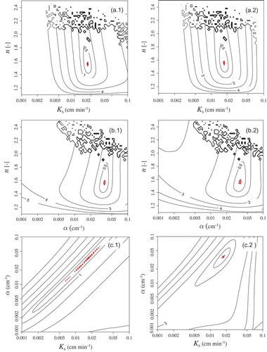
The response surfaces Φ(K_s,n), Φ(α,n) and Φ(K_s,α) calculated for the theoretical loam soil and the five different scenarios, Cap0, Cap0 + h, Evap, Cap0 + Evap and Cap0 + h + Evap, are shown in Figures 2–4. For the Cap0 case, the results showed that the α_w and K_s parameters were relatively well defined in the K_s–n and α_w–n response surfaces; however, the elongated vertical minimum found in these planes indicated that multiple combinations of the n values within this contour region yielded almost identical curves (Fig. 2(a.1) and (b.1)). However, the valley shape observed in the K_s–α_w plane (Fig. 2(c.1)) indicated that it is not possible to estimate the α_w and K_s parameters. Thus, we can conclude that these measurements were not adequate to uniquely define the soil hydraulic parameters. Other authors (Russo et al. 1991, van Dam et al. 1992, Eching and Hopmans 1993, Simunek and van Genuchten 1996, 1997) found similar results when analysing a one-step outflow coming from a cumulative infiltration experiment, or applying a one-step upward infiltration process (Moret-Fernández et al. 2016). In the second scenario, Cap0 + h (Fig. 2(a.2), (b.2) and (c.2)), only the K_s–α_w plane (Fig. 2(c.2)), showed a unique and well-defined minimum; however, the absence of methods to independently estimate the n parameter made it impossible to estimate K_s and α_w from an upward infiltration process followed by an overpressure step. Analysis of the third scenario (Evap) showed that only the n parameter was relatively well defined in the K–n and K–α_d contour maps (Fig. 3). Although K_s could easily be determined by Darcy’s law from an overpressure step on a saturated soil sample, the high uncertainty observed in the α_d parameter within the α_d–n plane, made it necessary to reject the evaporation process as a method to estimate soil hydraulic properties. The contour maps, however, changed greatly when both the upward infiltration and evaporation curves were first simulated separately and subsequently joined in a single curve (Cap0 + Evap) (Fig. 4(a)). Under this scenario, only the contour maps for the K–n and the α_w–n planes showed a unique and well-defined minimum (Fig. 4(a.1) and (b.1)). For practical purposes, due to the fact that K_s can easily be estimated by Darcy’s law by means of an overpressure step at the end of the wetting process, the method based on the measurement of upward infiltration followed by an evaporation process may prove to be a suitable tool to estimate soil hydraulic parameters. This statement is clear in the fifth scenario, Cap0 + h + Evap, where a unique and well-defined minimum was observed in all planes of the contour maps (Fig. 4(b)). The deviations between the theoretical α_w and n values and those estimated with the Cap0 + h + Evap method were 0.62% (log scale) and 0.615 %, respectively. From these results, we can conclude that, among the five different scenarios presented, the optimization method based on the measurement of an upward infiltration curve plus an overpressure step followed by an evaporation process (Cap0 + h + Evap) was the unique combination of curves that allowed accurate estimates of soil hydraulic properties. However, from a practical standpoint, we consider that a more effective way to determine soil hydraulic properties could be:

• Measurement of the cumulative upward infiltration curve with saturation conditions at the bottom of the soil sample.

• Application of an overpressure step at the end of the soil wetting process. This allows determination of K_s by Darcy’s law (Equation (9)).

• Measurement of the cumulative evaporation curve of the saturated soil sample at a constant evaporation rate until the soil reaches a constant weight.

• Measurement of the potential evaporation rate from the slope of the first phase of the cumulative evaporation curve.

• Synthetic fusion of the measured cumulative upward infiltration water (without the overpressure step) and the corresponding cumulative evaporation curve.

• Using the previously calculated K_s value, minimization of the objective function (Equation (10)) for the Cap0 + h + Evap scenario regarding the experimental curve in the α_w–n plane.

Figure 2. Contours of the objective function Φ(K,α,n) for the upward infiltration curves in the (a) K–n, (b) α–n and (c) K–α planes, without (1) and with (2) an overpressure step of 5 cm at the end of the wetting process. The number of contour lines corresponds to a 70 × 70 parameter combination grid. The thick (red) line indicates the experimental contour line corresponding to a RMSE of 0.1 mm due to water level measurement.

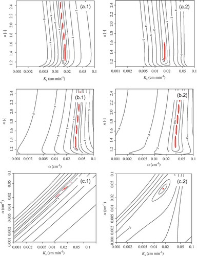
Figure 3. Contours of the objective function Φ(K,α,n) for an evaporation process: one parameter is fixed and the other two are optimized in the (a) K–n, (b) α–n and (c) K–α planes. See Figure 2 caption for details.

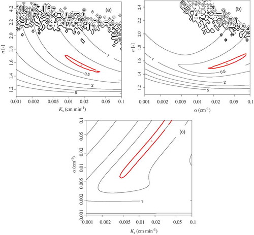
Figure 4. Contours of the objective function Φ(K,α,n) for the upward infiltration curves plus the cumulative evaporation curves: one parameter is fixed and the other two are optimized in the (a) K–n, (b) α–n and (c) K–α planes, without (a) and with (b) an overpressure step of 5 cm at the end of the wetting process. See Figure 2 caption for details.

3.2 Experimental testing

Following the conclusion described in Section 3.1, from here on, only the Cap0 + h + Evap method was tested on the experimental soils. To this end, the K_s calculated with Darcy’s law and the subsequent minimization of the objective function in the α_w–n the plane were used in the procedure. Table 3 shows values of the measured soil bulk density (ρ_b), saturated (θ_s) and residual (θ_r) water content, the saturated hydraulic conductivity measured by Darcy’s law, and the α_d and n values measured with the TDR pressure cell and those estimated with the Cap0 + h + Evap method (α_w and n parameters), on sand and 2-mm sieved loam and clay-loam soils.

Table 3. Soil bulk density (ρ_b), saturated (θ_s) and residual water contents (θ_r), saturated hydraulic conductivity (K_s), the n and α parameters of the van Genuchten (1980) water retention curve estimated for a wetting (α_w) and a draining process (α_d) from the TDR-pressure cell (PC) and the inverse analysis (CR-E), respectively, measured on sand and 2-mm sieved loam and clay-loam soils. The α values in italics were calculated according to the Gebrenegus and Ghezzehei (2011) model. W & D: wetting and drying.

				θs (cm^3 cm^−3)
Soil	Method	Process	ρb (g cm^−3)	Wetting	Drying	θr(cm^3 cm^−3)	Ks (cm min^−1)	αw(cm^−1)	αd(cm^−1)	n [-]
Fine sand	PC	Draining	1.57	-	0.38	0.020	-	0.1081	0.054	2.33
	CR-E	W & D	1.60	0.378	0.42	0.001	0.6486	0.07406	0.037	2.6
Loam	PC	Draining	1.19	-	0.48	0.150	-	0.076	0.039	1.64
	CR-E	W & D	1.09	0.43	0.53	0.012	0.0969	0.0905	0.0468	1.52
Clay-loam	PC	Draining	1.31	-	0.52	0.360	-	0.102	0.055	1.32
	CR-E	W & D	1.26	0.54	0.52	0.008	0.0476	0.0741	0.0383	1.52

As an example, analysis of the error map for the α_w–n plane calculated for the 2-mm sieved loam soil showed a unique and well-defined minimum, which indicates that is possible to accurately estimate soil hydraulic properties (Fig. 5(a)). These results are clear in the good agreement between the best-optimized and experimental curves (Fig. 5(b)). The a_d and n values estimated in all experimental soils using the inverse analysis were of the same order of magnitude as those measured using the TDR-pressure cells (Table 3). Although not significant (p = 0.2), a relationship with slope close to 1 was found between the measured and modelled n values (r = 0.9039). Overall, the deviation between the α_d (in logarithmic scale for all soils) and n values measured with the TDR pressure cell and the inverse analysis method were 12.95 and 7.32, 5.62 and 7.32, and 12.47 and 13.16%, for the sand, loam and clay-loam soils, respectively. Figure 6 shows the agreement between the θ(h) curves measured with the TDR-pressure cells in sand, sieved loam and sieved clay-loam soils, and those estimated with the Cap0 + h + Evap method.

Figure 5. (a) Contours of the objective function Φ(K,α,n) for the cumulative upward infiltration plus the cumulative evaporation curves: one parameter is fixed and the other two are optimized in the α–n plane for a 2-mm sieved loam soil. See Figure 2 caption for details. (b) Experimental (circles) and optimized simulated (line) cumulative upward infiltration plus evaporation curves measured on a 2-mm sieved loam. (WCR: water capillary rise.)

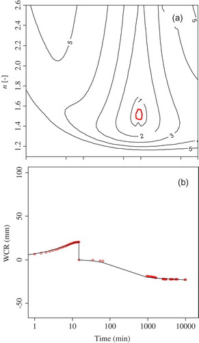
Figure 6. Comparison between effective saturation (S_e) curves measured in (a) fine sand, (b) sieved loam and (c) sieved clay-loam soil with TDR pressure cells (circles) during a draining process and the corresponding curve obtained by inverse analysis (line) of the cumulative upward infiltration–evaporation curve in the draining branch of the water retention curve.

4 Conclusions

This work presents an alternative method to estimate soil hydraulic parameters (K_s, α and n) from the inverse analysis of a cumulative upward infiltration curve plus an overpressure step followed by a cumulative evaporative process (Cap0 + h + Evap). Using the HYDRUS 2D model, the method was tested on a theoretical loam soil under the following scenarios: (a) an upward infiltration wetting process at saturation (Cap0); (b) an evaporation process (Evap); (c) an upward infiltration wetting process at saturation followed by an evaporation one (Cap0 + Evap); (d) and (e) the Cap0 and Cap0 + Evap with and without overpressure step (h) at the end of the wetting simulations. The method was next tested in the laboratory on sand and 2-mm sieved loam and clay-loam soils. The Cap0 + h + Evap curve was the unique scenario that allowed accurate estimations of soil hydraulic properties. As a practical method, we propose calculating K_s by means of Darcy’s law and minimization of the objective function in the α_w–n error map plane. A satisfactory validation of this method was also obtained from the laboratory experiments. Although the results were acceptable, the method, which needs several days to make the measurements, was very sensitive to the water content at saturation and to the initial water content in the evaporation simulations. Thus, care should be taken when measuring these parameters. Compared to existing techniques used to estimate θ(h), the method proposed here is simple to implement, allows sweeping of a whole range of soil tensions, does not need tensiometers, can be applied on standard soil bulk density cylinders (i.d.: 5 cm; height: 5 cm); could be multiplied if several balances are used simultaneously; and it has been successfully applied in different textural soils. However, further research is needed to (i) reduce the calculation time by using more efficient optimization techniques (i.e. Bayesian methods); (ii) test the method on more soil textural classes, possibly spanning all the 12 USDA textural classes; (iii) test the method on undisturbed soil samples; and (iv) test the method with alternative soil hysteresis models.

Acknowledgements

The authors are grateful to Josefa Salvador, Ricardo Gracia and Victoria López for their technical support in developing this work.

Disclosure statement

No potential conflict of interest was reported by the authors.

Additional information

Funding

This research was supported by the Spanish Ministry of Economy and Competitiveness (grants AGL2010-22050-CO3-02/AGR and BES-2011-076839).

References

- Arya, L.M., 2002. Wind and hot-air methods. In: J.H. Dane and G.C. Topp, eds. Methods of soil analysis. Part.4. Madison, WI: Soil Science Society of America Book Series No. 5.
- Carsel, R.F. and Parrish, R.S., 1988, Developing joint probability distributions of soil water retention characteristics. Water Resources Research, 24, 755–769.
- Casey, F.X.M. and Derby, N.E., 2002, Improved design for an automated tension infiltrometer. Soil Science Society of America Journal, 66, 64–67.
- Dane, J.H. and Hopmans, J.W., 2002. Water retention and storage. In: J.H. Dane and G.C. Topp, eds. Methods of soil analysis. Part.4. Madison, WI: Soil Science Society of America Book Series No. 5.
- Eching, S.O. and Hopmans, J.W., 1993, Optimization of hydraulic functions from transient outflow and soil water pressure data. Science Society of America Journal, 57, 1167–1175.
- Gebrenegus, T. and Ghezzehei, T.A., 2011, An index for degree of hysteresis in water retention. Soil Science Society of America Journal, 75, 2122–2127.
- Green, W.H. and Ampt, G.A., 1911, Studies in soil physics, part I: the flow of air and water through soils. Journal of Agricultural Science, 4, 1–24.
- Ippisch, O., et al., 2006. Validity limits for the van Genuchten-Mualem model and implications for parameter estimation and numerical simulation. Advances in Water Resources, 29, 1780–1789.
- Klute, A., 1986. Water retention curve: laboratory methods. In: A. Klute, ed. Methods of soil analysis. Part 1. Madison WI: Soil Science Society of America Book Series No. 9.
- Lichtner, P.C., Steefel, C.I., and Oelkers, E.H., 1996. Reactive transport in porous media. Denver, CO: Mineralogical Society of America, 5. ISBN 0-939950-42-1.
- Likos, W.J., et al., 2014. Hysteresis and uncertainty in soil water-retention curve parameters. Journal of Geotechnical and Geoenvironmental Engineering. doi:10.1061/(ASCE)GT.1943-5606.0001071
- Mboh, C.M.E.A., 2011, Feasibility of sequential and coupled inversion of time domain reflectometry data to infer soil hydraulic parameters under falling head infiltration. Soil Science Society of America Journal, 75, 775–786.
- Mohammadzadeh-Habili, J. and Heidarpour, M., 2011, Estimating soil hydraulic parameters by using Green and Ampt infiltration equation. Journal of Hydrologic Engineering, 16, 772–780.
- Moret-Fernández, D., et al., 2012. TDR pressure cell for monitoring water content retention and bulk electrical conductivity curves in undisturbed soil samples. Hydrological Processes, 26, 246–254.
- Moret-Fernández, D., et al., 2016. A modified tension upward infiltration method to estimate the soil hydraulic properties. Hydrological Processes. (wileyonlinelibrary.com) doi:10.002/hyp.10827
- Mualem, Y., 1976, A new model for predicting the hydraulic conductivity of unsaturated porous media. Water Resources Research, 12, 513–522.
- Munkholm, L.J. and Kay, B.D., 2002, Effect of water regime on aggregate-tensile strength, rupture energy, and friability. Soil Science Society of America Journal, 66, 702–709.
- Pardalos PM, Romeijn HE., Eds. 2002. Handbook of global optimization (vol. 2). Dordrecht: SpringerScience+BusinessMedia. doi:10.1007/978-1-4757-5362-2.
- Rashid, N.S.A., et al., 2015. Inverse estimation of soil hydraulic properties under oil palm trees. Geoderma, 241-242, 306–312.
- Reynolds, W.D., 2002. Saturated and field-saturated water flow parameters. In: J.H. Dane, et al., eds. Methods of soil analysis. Part.4. Madison, WI: Soil Science Society of America Book Series No. 5.
- Russo, D., et al., 1991. Analysis of infiltration events in relation to determining soil hydraulic properties by inverse problem methodology. Water Resources Research, 27, 1361–1373.
- Seki, K., 2007, SWRC fit – a nonlinear fitting program with a water retention curve for soils having unimodal and bimodal pore structure. Hydrology and Earth System Sciences, 4, 407–437.
- Simunek, J., et al., 1998. Parameter estimation analysis of the evaporation method for determining soil hydraulic properties. Soil Science Society of America Journal, 62, 894–895.
- Simunek, J., et al., 2001. Non-equilibrium water flow characterized by means of upward infiltration experiments. European Journal of Soil Science, 52, 13–24.
- Simunek, J. and van Genuchten, M.T., 1996, Estimating unsaturated soil hydraulic properties from tension disc infiltrometer data by numerical inversion. Water Resources Research, 32, 2683–2696.
- Simunek, J. and van Genuchten, M.T., 1997, Estimating unsaturated soil hydraulic properties from multiple tension disc infiltrometer data. Soil Science, 162, 383–398.
- Simunek, J., van Genuchten, M.T., and Sejna, M., 2008, Development and applications of the HYDRUS and STANMOD software packages and related codes. Vadose Zone Journal, 7 (2), 587–600.
- van Dam, J.C., et al., 1992. Inverse method for determining soil hydraulic functions from one-step outflow experiment. Soil Science Society of America, 56, 1042–1050.
- van Genuchten, M.T., 1980, A closed-form equation for predicting the hydraulic properties of unsaturated soils. Soil Science Society of America Journal, 44, 892–898.
- Vogel, T., van Genuchten, M.T., and Cislerová, M., 2001, Effect of the shape of the soil hydraulic functions near saturation on variably-saturated flow predictions. Advances in Water Resources, 24 (2), 133–144.
- Wand, X., and Benson, C.H., 2004, Leak-free pressure plate extractor for measuring the soil water characteristic curve. Geotechnical Testing Journal, 27, 1–9.
- Wendroth, O., et al., 1993. Reevaluation of the evaporation method for determining hydraulic functions in unsaturated soils. Soil Science Society of America Journal, 57, 1436–1443.
- Wind, G.P., 1968. Capillary conductivity data estimated by a simple method. In: P.E. Rijtema and H. Wassink, eds. Water in the unsaturated zone. Gentbrugge, Belgium: IASAH, Proc. Wageningen Symp. June 1966. Vol. 1, 181–191.
- Young, M.H., Karagunduz, A., and Simunek, J., 2002, A modified upward infiltration method for characterizing soil hydraulic properties. Soil Science Society of America Journal, 66, 57–64.