Use of ACRU, a distributed hydrological model, to evaluate how errors from downscaled rainfall are propagated in simulated runoff in uMngeni catchment, South Africa

ABSTRACT

The hypothesis of no significant difference in errors between observed (historical) and downscaled global circulation model (GCM) rainfall and corresponding errors in simulated runoff was tested. The percentage difference in mean and standard deviation, normalized errors and normalized bias metrics were used. The ACRU hydrological model was used to simulate runoff. Results indicated that errors in rainfall lead to amplified errors in simulated runoff. A 10% error magnitude in mean rainfall was amplified three times in mean runoff. Rainfall variability was amplified by twice as much from rainfall to simulated runoff. These findings indicate that uncertainty in input downscaled rainfall is amplified in simulated runoff, hence the quality of input rainfall is a strong determining factor of the simulated runoff. Ultimately, there is a need for continuous improvement in the GCM downscaling process, particularly model process description, so as to minimize uncertainties due to GCM model description.

EDITOR A. Castellarin; ASSOCIATE EDITOR S. Kanae

KEYWORDS:

• error propagation
• downscaled climate models
• input data uncertainty
• rainfall
• runoff

1 Introduction

Several studies in southern Africa have reported on hydrological responses to climate change using rainfall–runoff models (e.g. Hughes 2004, 2013, Schulze 2005, Hughes et al. 2010, Graham et al. 2011). Modelling is, however, an inherently probabilistic exercise, with uncertainty amplified at each stage of the modelling process (Praskievicz and Chang 2009). Among the obvious sources of errors in the modelling process are errors associated with the model inputs, model structure, and parameters /variables and boundary conditions (Beven 2011). Overall, uncertainties in rainfall play a significant role in hydrological modelling, since they constitute the main driving force for the hydrological cycle (Hostache et al. 2011). Predictive uncertainty, however, is a result of several uncertainty sources (input, parameter, model structure) interacting with each other (Liu and Gupta 2007), as illustrated in Figure 1.

Figure 1. The uncertainty envelope in hydrology showing the uncertainty sources from input uncertainty, model structure uncertainty and parameter uncertainty.

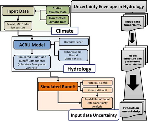
It has been established that input data uncertainty, in particular uncertainty associated with rainfall data input, affects the total simulation uncertainty significantly (Andréassian et al. 2001, Pappenberger et al. 2005). The majority of climate impact studies also make the assumption that the use of more global circulation models (GCMs), to a greater extent, enables the full representation of the uncertainty envelope (Honti et al. 2014, Zhang et al. 2014). To date, this has been enabled by the availability of downscaled GCM climate data representing plausible different climate scenarios, covering watersheds at finer spatial scales (Tadross et al. 2005, Hewitson and Crane 2006, Hewitson and Tadross 2011). It has also been established that the greatest uncertainties in the effect of climate on runoff arise from uncertainties in climate change scenarios, as long as a conceptually sound hydrological model is used (Gosling et al. 2011, Najafi et al. 2011, Arnell and Gosling 2013,). The range of runoff output from hydrological modelling driven by different downscaled GCM climate data can thus be presented as an indication of uncertainty from GCMs, and hence the magnitude of errors propagated from input rainfall data.

Several hydrological metrics have been used in other world regions in assessing uncertainty propagation from rainfall to simulated runoff (see e.g. Pappenberger et al. 2005, Borga et al. 2006, Nikolopoulos et al. 2010, Zhu et al. 2013). Such studies have shown that uncertainty propagation is dependent on several factors including basin size, magnitude of input rainfall error and the type of hydrological model used, among others. For instance, Borga (2002), in southwest England, found that mean absolute error ranged from zero up to 0.60 when runoff simulated using radar-generated rainfall was compared to runoff simulated using historical rainfall, showing that rainfall errors are propagated through to simulated runoff. Using normalized errors and normalized bias to analyse the uncertainty propagation from radar rainfall to simulated runoff, Zhu et al. (2013) showed that normalized bias of the radar rainfall estimates was enhanced in simulated stream flow, particularly when the rainfall normalized bias was above zero. However, Zhijia et al. (2004), using the mean field bias, found that the relative differences between radar and historical rainfall ranged from 9.95 to 14.25%. However, no significant differences in the runoff from the two data sets were observed. It was concluded that there was no linear relationship between errors in input rainfall and errors in simulated runoff (Zhijia et al. 2004). On the other hand, Nikolopoulos et al. (2010), using the relative error to investigate the propagation of uncertainty in satellite radar rainfall through the rainfall–runoff transformation, established that the propagation of uncertainty exhibited not only a linear behaviour, especially for the larger-scale basins, but was also dependent on the basin size, such that the error dampening reduced as the basin scale increased.

Other studies have used different metrics for the study of rainfall error propagation in hydrological modelling (e.g. Moulin et al. 2009, Chiew et al. 2010, Vaze et al. 2010, Teng et al. 2012). These studies established that, among other factors (e.g. catchment size, choice of GCM model, seasonal rainfall distribution), errors due to input rainfall accounted for a significant amount of error propagation relative to the model and parameter uncertainty. For example, Moulin et al. (2009) used Monte Carlo simulations to simulate error scenarios, which were then used to drive two calibrated hydrological models. They showed that a large part of the hydrological modelling errors could be explained by the uncertainties in rainfall estimates. Chiew et al. (2010) used several runoff characteristics, such as mean annual runoff, mean summer (December–January–February) runoff, mean winter (June–July–August) runoff, inter-annual variability of annual runoff, extreme high daily runoff and a low flow characteristic, to compare the runoff distributions. The study established that mean annual and summer runoff modelled using daily rainfall from the analogue model downscaled from the CSIRO GCM were also underestimated, consistent with the underestimation of the mean annual and summer rainfall. This approach further showed the influence of the GCM choice as well as the rainfall seasonality.

Even though, as shown above, a range of international literature on input data uncertainty as well as error propagation is available, few studies have been carried out in southern Africa (e.g. Sawunyama and Hughes 2008, Kapangaziwiri et al. 2012, Hughes et al. 2014, Hughes 2016). In all the above studies, input data were used to drive a monthly step hydrological model, the Pitman model. This study, on the other hand, was aimed at evaluating input data uncertainty propagation using a daily time step physical conceptual model, the ACRU hydrological model. The major drawback in using monthly time step models is that climate change will alter not only the magnitude but also the timing of hydrological events that might not be captured by monthly step models, such as the Pitman. Results from an earlier study by Kusangaya et al. (2016) showed that the downscaled rainfall projections do not seem to adequately capture the range of rainfall events required for hydrological understanding. The emerging question is thus: What then is the added uncertainty in simulated runoff when using the downscaled rainfall projections as input in hydrological modelling? Research undertaken here was aimed at evaluating if errors in downscaled GCM rainfall are typically propagated or amplified in simulated runoff. The error propagation was evaluated using statistical measures of error, bias and percentage change properties of projected rainfall and of the simulated runoff data series.

2 Materials and methods

Different hydrological metrics have been used in analysing error propagation from rainfall to runoff. Relatively simple measures of streamflow conditions (e.g. mean, median, maximum, minimum flows) are often used. For this study, key rainfall and runoff characteristics, for the time period 1961–1999, denoting the mean and variability were examined to determine if errors in downscaled rainfall were propagated and amplified in the resultant simulated runoff. The ACRU model was used to simulate runoff for the uMngeni catchment under the baseline land cover of Acocks (1988) Veld Types, using historical observed climate data and downscaled GCM climate data.

2.1 Study area

The uMngeni catchment (4349 km²), divided into 13 water management areas (WMAs), namely Mpendle, Lions River, Midmar, Henley, Albert Falls, Pietermaritzburg, Karkloof, New Hanover, Nagle, Table Mountain, Mqeku, Inanda and Durban, is located in the KwaZulu-Natal province of South Africa (Fig. 2). The altitude in the catchment ranges from 1913 m a.s.l. in the western escarpment of the catchment to sea level at the catchment’s outlet into the Indian Ocean. The mean annual precipitation (MAP) of the catchment varies from 1550 mm p.a. in the main water source areas in the west of the catchment to 700 mm p.a. in the drier middle reaches of the catchment (Summerton and Schulze 2009, Summerton et al. 2009). The rainfall throughout the catchment is, however, highly variable, both inter- and intra-annually. The mean annual potential evaporation ranges from 1 567 mm p.a. to 1 737 mm p.a. The mean annual temperature ranges from 12°C in the escarpment areas to 20°C towards the coastal areas of the catchment (Summerton et al. 2009).

Figure 2. Location of the uMngeni catchment in KwaZulu-Natal Province, South Africa, showing the 13 water management areas (WMAs) and the Acocks Veld Types (Acocks 1988).

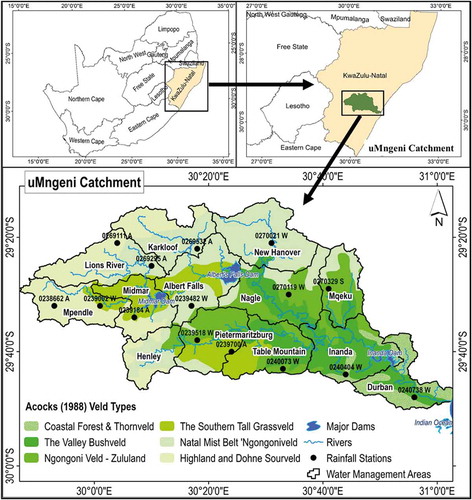
The uMngeni catchment supplies water to nearly 15% of South Africa’s population. It is thus important to understand the uncertainty in the runoff projections for the catchment. Additionally, given the water-stressed nature of the catchment and the ongoing studies around climate change adaptation and policy, it was considered a key catchment to assess. Additionally, previous climate change impacts on hydrology studies in the same catchment (e.g. Tarboton and Schulze 1992, Summerton 2008, Summerton et al. 2009, 2010, Warburton et al. 2010, 2012) did not explicitly consider the uncertainty in downscaled climate data and hydrological simulations.

2.2 Historical rainfall data and downscaled GCM climate data

Historical rainfall data were obtained for 13 rainfall stations in the uMngeni catchment, and compared to the rainfall output from 10 downscaled GCMs, for the time period 1961–1999. There was at least one rainfall station in each of the 13 WMAs of the uMngeni catchment and therefore the rainfall from the particular station in a WMA was taken as being representative of the rainfall received for that particular WMA. Downscaled climate model data were obtained from the Climate System Analysis Group at the University of Cape Town (CSAG–UCT). The climate models were statistically downscaled from the fifth phase of the Coupled Model Inter-comparison Project (CMIP5). These were downscaled to each of 13 rainfall stations from which historical data were obtained. Table 1 summarizes the characteristics of the 10 selected downscaled GCM climate datasets. Rainfall and temperature data from the climate models were used to drive the ACRU model and generate the runoff that was analysed in this study.

Table 1. Downscaled climate models from CSAG – UCT that were used in this study to compare against historical rainfall and also to simulate runoff.

GCM	Country of origin	Host organization	Acronym (for this study)	Variables downscaled	Periods
CCCMA_CGCM3.1	Canada	Canadian Centre for Climate Modelling & Analysis (CCCMA)	cc1	rainfall
				max. temp.	1961–1999
				min. temp.
CNRM_CM3	France	Centre National de Recherches Météorologiques, Météo France (CNRM)	cn1	rainfall	1961–1999
				max. temp.
				min. temp.
MIUB_ECHO_G	Germany and Korea	Meteorological Institute of the University of Bonn (MIUB, Germany) and Institute of KMA (Korea) and Model and Data Group	e11	rainfall	1961–1999
				max. temp.
				min. temp.
MPI_ECHAM5	Germany	Max Planck Institute for Meteorology (MPI)	e12	rainfall	1961–1999
				max. temp.
				min. temp.
GISS-E-R	USA	NASA Goddard Institute for Space Studies (NASA/GISS)	gi1	rainfall	1961–1999
				max. temp.
				min. temp.
IPSL-CM4	France	Institut Pierre Simon Laplace (IPSL)	ip1	rainfall	1961–1999
				max. temp.
				min. temp.
CSIRO_MK3_5	Australia	Commonwealth Scientific and Industrial Research Organization (CSIRO)	cs1	rainfall	1961–1999
				max. temp.
				min. temp.
GFDL_CM2_0	USA	Geophysical Fluid Dynamics Laboratory, NOAA (GFDL)	g11	rainfall	1961–1999
				max. temp.
				min. temp.
GFDL-CM2.1	USA	Geophysical Fluid Dynamics Laboratory, NOAA (GFDL)	g12	rainfall	1961–1999
				max. temp.
				min. temp.
MRI_CGCM2_3_2A	Japan	Meteorological Research Institute, Japan Meteorological Agency (MRI)	mr1	rainfall	1961–1999
				max. temp.
				min. temp.

2.3 The ACRU hydrological modelling system

The ACRU hydrological model, developed by Schulze (1995), is a daily time step process-based model with a multi-soil-layer water budget, which is sensitive to land management and changes thereof, as well as to climate input and changes (Smithers and Schulze 1995, Smithers et al. 1997, Schulze and Perks 2000). The model is designed to simulate daily, monthly and annual soil water budgets for use in agro-hydrological applications. The generation of runoff in ACRU is based on the premise that, after initial abstractions (through interception, depression storage and infiltration before runoff commences), the runoff produced is a function of the magnitude of the rainfall and the soil water deficit from a critical response depth of the soil (Schulze 1995).

The ACRU model is not a model in which parameters are calibrated to produce a good fit; rather, values of input variables are estimated from the physical characteristics of the catchment (Smithers and Schulze 1995). The configuration of the ACRU model used in this study was done by Warburton et al. (2010) in a confirmation study of the use of ACRU for climate impact studies for the uMngeni catchment. Warburton et al. (2010) showed that the ACRU model can be used successfully for climate change impact studies in a study on three diverse South African catchments with diverse land uses and different climate regimes. Furthermore, the ACRU model has been applied extensively for climate change impact studies (e.g. Tarboton and Schulze 1992, Schulze and Perks 2000, Schulze et al. 2003, Schulze 2005, 2011, Warburton et al. 2005, 2012, Graham et al. 2011, Kienzle et al. 2012). The ACRU model has been applied widely in southern Africa for both land use and climate change impact studies, and it was thus hypothesized that the ACRU model structure is adequate and any propagation errors were derived largely from the input rainfall. Therefore, the ACRU model was adopted for this study to generate runoff using the historical “observed” daily climatic records, as well as using the different downscaled GCM daily climate data.

The Acocks Veld Type maps (Acocks 1988) were used as a baseline land cover input to the ACRU model, to simulate streamflow responses that would occur under natural land cover. The Acocks Veld Type maps are the most scientifically respected and generally accepted maps of natural vegetation for South Africa. Estimates of streamflow responses from the Acocks Veld Types have formed the basis on which streamflow reductions due to land use change, as outlined in the South African National Water Act (NWA 1998), have been assessed since 1998 (Gush et al. 2002) and, more recently, streamflow changes due to climatic changes (Warburton et al. 2012).

According to Warburton et al. (2012), soil information for input for the ACRU model was obtained from the electronic data accompanying the South African Atlas of Climatology and Agrohydrology (Schulze 2011). Such information included thickness of the topsoil and subsoil, as well as soil water content at the soil’s lower limit (i.e. permanent wilting point), its drained upper limit (i.e. field capacity) and saturation for both the topsoil and subsoil. Explicit details on soil information requirements for the ACRU model can be obtained from Schulze (1995).

In order to simulate runoff, the hydro-climatological requirements of the ACRU model are daily rainfall and daily reference evaporation (A-pan equivalent) data. In the ACRU model, daily reference evaporation is computed from daily minimum and maximum temperatures if A-pan reference evaporation data are not available. As daily A-pan evaporation records were not available for the uMngeni WMAs, the Hargreaves and Samani (1985) daily A-pan equivalent reference evaporation equation, which is an option in the ACRU model, was used to estimate the daily reference evaporation. Bezuidenhout (2005) found that the Hargreaves and Samani (1985) equation mimicked the daily reference evaporation values well for South Africa. Historical “observed” daily temperatures, which were used for the reference evaporation calculation, were extracted from a gridded database of daily temperatures for South Africa (see Schulze and Maharaj 2004) for the centroid of each WMA for the period 1961–1999 (for details, see Warburton et al. 2010). These historical daily temperature values were used to estimate the reference evapotranspiration, in ACRU, for runoff simulation using the historical “observed” climatic data. Similarly, the minimum and maximum temperatures of the different GCMs were used to estimate the GCM reference evapotranspiration, in ACRU, for runoff simulation using the different GCMs for the historical time period (1961–1999).

2.4 Rainfall–runoff hydrological error propagation metrics

Five metrics were selected as suitable for use in analysing both rainfall and runoff error propagation, namely percentage difference in mean (dM), percentage difference in standard deviation (dSD), percentage difference of coefficient of variation (dCV), normalized error and normalized bias. These metrics were calculated using daily rainfall and runoff records. The metrics were selected because of their simplicity of use, hence they are widely used (e.g. Bringi et al. 2001, Hossain et al. 2004, Gabellani et al. 2007, Zhu et al. 2013). The first three metrics work well under the assumption of data normality, whilst the last two are distribution-free statistics. Since the data length was reasonably long (40 years), it was assumed that results from the metrics should complement each other and show the same trends since, according to Gorard (2005), efficiency of normalized errors/normalized bias is at least as good as standard deviation/variance for non-normal distributions. The five metrics were therefore considered both “sufficient” and “efficient” measures of error propagation. More specifically, they are considered “sufficient” in the sense of summarizing all of the relevant information to be gleaned from the rainfall and runoff over sufficiently long periods, and “efficient” in the sense of having the smallest probable error as an estimate of the data long-term trends. The dM, dSD and dCV were derived as follows:

(1)

(2)

(3)

where X_ro is the observed daily rainfall (or daily runoff simulated using observed rainfall); X_rd is the downscaled daily rainfall (or daily runoff simulated using downscaled rainfall); is the mean of observed daily rainfall (or mean of daily runoff simulated using observed rainfall); is the mean of downscaled daily rainfall (or mean of daily runoff simulated using downscaled rainfall); is the standard deviation of daily observed rainfall (or standard deviation of daily runoff simulated using observed rainfall); is the standard deviation of daily downscaled rainfall (or standard deviation runoff simulated using downscaled rainfall).

Further analysis of error propagation was carried out using normalized errors and normalized bias following approaches adapted from Bringi et al. (2001), Hossain et al. (2004) and Zhu et al. (2013), who used these metrics in statistical analysis of error propagation from radar rainfall to simulated runoff. Gabellani et al. (2007) used the same metrics in analysing error propagation from rainfall to runoff. Rainfall error was defined as the relative difference between the observed historical rainfall and rainfall simulated from downscaled GCMs. Likewise, the runoff error was defined as the relative difference between runoff simulated using observed historical climate data vs runoff simulated using downscaled climate data. Normalized error (NE) and normalized bias (NB) were used to calculate the rainfall:runoff error propagation; the equations are as follows:

(4)

(5)

where n is the total number of observations and other variables as are in Equations (1)–(3).

Historical rainfall data were taken as the reference data, represented by X_ro (Equations (1), (3) and (4)), whereas the downscaled rainfall data were denoted by X_rd. Using the same equations to calculate the differences in runoff, the simulated runoff derived from observed rainfall data were denoted by X_ro and the corresponding simulated runoff from downscaled rainfall was denoted by X_rd.

3 Results

Errors in downscaled rainfall were amplified in simulated runoff. The magnitude of the error propagation differed from one WMA to another, as well as from one GCM to another. Overall, there was an average of a 1:3 error propagation in mean rainfall: runoff, implying that a 10% error magnitude in mean rainfall was amplified three times in mean runoff. However, errors in variability (standard deviation, SD, and coefficient of variation, CV) were amplified two-fold from rainfall to runoff. This implied that a 10% error in rainfall variation was amplified into a 20% magnitude error in simulated runoff variability, on average.

3.1 Confirmation of the ACRU model

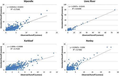
Warburton et al. (2010) showed that, overall, the ACRU model performed well on each of the four WMAs included in the confirmation study (Fig. 3 and Table 2). The results showed that the ACRU model can be used to simulate streamflows of the uMngeni catchment, with reasonable confidence. For example, for the Mpendle WMA, the total flows were adequately simulated, the percentage difference between the observed and simulated standard deviation was found to be less than 15%, the R² of daily values was 0.836 and the Nash-Sutcliffe efficiency criterion, E_f, was 0.802. Therefore, simulation of streamflow in the Mpendle WMA was considered highly acceptable. The Lions River WMA, in contrast, similarly produced acceptable results with an R² of 0.882 (Table 2). For the Karkloof WMA, the Nash-Sutcliffe E_f of 0.655 and the other statistics (Table 2) were also considered acceptable. The results of the confirmation study for the Henley WMU were considered reasonable, as all statistics except for the percentage difference between the standard deviations were acceptable, and comparison of daily simulated and observed streamflows indicated that the variability of streamflow was adequately simulated (Fig. 3 and Table 2).

Table 2. Statistics of performance of the ACRU model, uMngeni catchment: comparison of daily historical and simulated values (Source: Warburton et al. 2010). SD: standard deviation.

WMA (1987–1998)	Mpendle	Lions River	Karkloof	Henley
Total observed flows (mm)	3444.068	2507.196	3456.985	2635.724
Total simulated flows (mm)	3171.486	2257.643	3005.969	2533.988
Average error in flow (mm/d)	−0.063	−0.058	−0.105	−0.024
Mean observed flows (mm/d)	0.796	0.582	0.803	0.629
Mean simulated flows (mm/d)	0.733	0.524	0.698	0.605
% difference between means	7.91%	9.95%	13.05%	3.86%
SD of observed flows (mm)	1.823	1.734	1.228	1.246
SD of simulated flows (mm)	2.011	1.947	1.305	1.541
% difference between SD	−10.34%	−12.31%	−6.26%	−23.67%
Correlation coefficient, Pearson’s R	0.915	0.939	0.844	0.886
Regression coefficient (slope)	1.009	1.055	0.897	1.095
Regression intercept	−0.07	−0.09	−0.022	−0.084
Coefficient of determination, R^2	0.836	0.882	0.713	0.785
Nash-Sutcliffe efficiency index, Ef	0.802	0.847	0.655	0.654

Figure 3. Statistics of performance of the ACRU model in uMngeni catchment: comparison of daily observed (historical) and simulated values.

3.2 Percentage difference in mean, standard deviation and coefficient of variation error propagation

The overall percentage difference in the mean for rainfall was approximately 5.3%, whilst for simulated mean runoff it was approximately −17.3%, showing an error propagation of 1:−3.3 from rainfall to runoff (Table 3). This implied that an error of 10% in mean rainfall was amplified by three times as much in simulated runoff. For example, for Pietermaritzburg WMA, a maximum negative percentage difference of −11% for rainfall mean and −35% for the simulated runoff mean was calculated, suggesting a rainfall:runoff error propagation of around 1:3. Nagle WMA, however, had a maximum negative ratio of error propagation of 1:−13. The negative bias in the percentage difference in mean rainfall:runoff – found in nine of the 13 WMAs (Table 3) – could be attributed to (a) the influence of extreme values, since when using the normalized mean, less negative bias (i.e. only in six of 13 WMAs, Table 4) was realized, or (b) other aspects of runoff generation, such as antecedent soil moisture conditions prevailing in preceding rainfall events. Table 3 shows the calculated error propagation from rainfall to runoff for the mean, SD and CV for the uMngeni catchment.

Table 3. Percentage difference of mean, standard deviation and coefficient of variation of rainfall and runoff for all the WMAs in uMngeni catchment, obtained using all the downscaled GCMs. SD: standard deviation; CV: coefficient of variation.

Percentage difference
WMAs	Mean rainfall	Mean runoff	Mean ratio	Rainfall SD	Runoff SD	SD ratio	Rainfall CV	Runoff CV	CV ratio
Mpendle	11	−21	1:−1.91	−55	−37	1:0.67	−59	−26	1:0.44
Lions River	5	−32	1:−6.4	−2	−28	1:14	−9	−6	1:0.67
Midmar	34	44	1:1.29	−1.2	−47	1:39.17	−28	−65	1:2.32
Karkloof	11	−17	1:−1.55	−6	−25	1:4.17	−36	−25	1:0.69
Albert Falls	10	−2	1:−0.2	−30	−49	1:1.63	−39	−55	1:1.41
Henley	54	104	1:1.93	−37	−20	1:0.54	−62	−67	1:1.08
Pietermaritzburg	−11	−35	1:3.18	−12	−66	1:5.5	−6	−53	1:8.83
New Hanover	−6	−31	1:5.17	−6	−28	1:4.67	−3	2	1:−0.67
Nagle	2	−25	1:−12.5	−25	−51	1:2.04	−30	−47	1:1.57
Table Mountain	−7	8	1:−1.14	−15	−39	1:2.6	−13	−51	1:3.92
Mqeku	7	−24	1:−3.43	−18	−43	1:2.39	−27	−36	1:1.33
Inanda	−4	3	1:−0.75	−22	−40	1:1.82	−20	−43	1:2.15
Durban	4	−15	1:−3.75	−2	−18	1:9	−12	−13	1:1.08
uMngeni average	5	−17	1:−3.4	−15	−39	1:2.6	−27	−43	1:1.59

Table 4. Rainfall to runoff error propagation ratio for the normalized errors (NE) and normalized bias (NB) for all the WMAs in uMngeni catchment.

WMA	Rainfall NE	Runoff NE	NE Ratio	Rainfall NB	Runoff NB	NB Ratio
Mpendle	0.31	0.66	1:2.13	0.11	−0.21	1:−1.91
Lions River	0.19	0.57	1:3	0.05	−0.32	1:−6.4
Midmar	0.39	0.99	1:2.54	0.34	0.44	1:1.29
Karkloof	0.21	0.52	1:2.48	0.11	−0.17	1:−1.55
Albert Falls	0.21	0.9	1:4.29	0.1	−0.02	1:−0.2
Henley	0.61	1.44	1:2.36	0.54	1.04	1:1.93
Pietermaritzburg	0.24	0.88	1:3.67	−0.11	−0.35	1:3.18
New Hanover	0.22	0.53	1:2.41	−0.06	−0.31	1:5.17
Nagle	0.2	0.98	1:4.9	0.02	−0.25	1:−12.5
Table Mountain	0.24	0.75	1:3.13	−0.07	0.08	1:−1.14
Mqeku	0.24	0.86	1:3.58	0.07	−0.24	1:−3.43
Inanda	0.28	1.04	1:3.71	−0.04	0.03	1:−0.75
Durban	0.25	0.69	1:2.76	0.04	−0.15	1:−3.75
uMngeni average	0.24	0.86	1:3.58	0.05	−0.17	1:−3.4

The percentage difference in standard deviation (dSD) for rainfall ranged from slightly above zero to maximum negative percentage difference of −55%, whilst that for runoff ranged from −18% to −66%. On the other hand, the percentage difference in CV ranged from −62% to −3%, and for simulated runoff from −67% to a maximum of 2%. Thus, for both the dSD and dCV the rainfall:runoff error propagation was on average around 1:2, implying that an error of 10% in SD in rainfall would be amplified twice as much in simulated runoff. All of the WMAs, however, had a negative bias in the percentage difference in standard deviation, which could be attributed to the influence of extreme values when using the standard deviation.

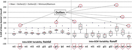
The Lions River, Midmar, Nagle and Durban WMAs had the highest error propagation (low rainfall error vs very high simulated runoff error) ranging from 1:−4 to 1:28. For example, in Midmar WMA, this was explained by the high variation within individual GCMs (Fig. 4), particularly GCMs cn1, g12, gi1 and ip1, which exhibited high intra-GCM variability characterized by data outliers. The extreme values (outliers) contributed significantly to the overall high error propagation values exhibited by the WMAs. For example, in the Midmar WMA, whilst the mean percentage difference error propagation was 1:1, the percentage difference of the standard deviation was as high as 1:120, showing the huge impact characteristic of outliers.

Figure 4. Intra-GCM variability of the mean, within Midmar WMA, showing GCMs (arrows) that were characterized by extreme values (circled outliers), which resulted in high error propagation.

3.3 Rainfall–runoff normalized errors and normalized bias

Table 4 and Figure 5 summarize the normalized bias and normalized error for uMngeni catchment, and show the error propagation from rainfall to runoff. The absolute normalized error for rainfall ranged from 0.19% to 0.61%, whilst for runoff it ranged from 0.52% to 1.44% (Table 4 and Fig. 5). The average normalized error for rainfall was therefore around 0.28% and for runoff around 0.83%, representing an error propagation ratio of 1:3 from rainfall to runoff. High error propagation ratio of 1:5 was evident in Nagle WMA, which was also characterized by high error propagation for the mean bias of 1:−12. Normalized bias ranged from −0.11% to 0.54% for rainfall and −0.35% to 1.04% for simulated runoff, with an average of 0.09% for rainfall and −0.03% for runoff.

Figure 5. Summary magnitude of rainfall:runoff ratios: (a) normalized error and (b) normalized bias from all the GCMs for all the WMAs of the uMngeni catchment.

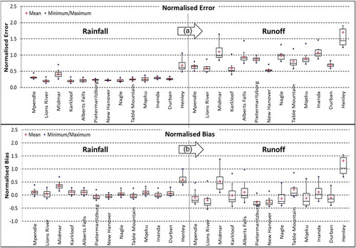
On average, the normalized error was around 1:3, implying that a 10% error in rainfall is magnified three times (30%) in simulated runoff. The same error amplification ratio was obtained from the percentage difference of the mean. Yet the mean bias exhibited an error propagation ratio of around 1:2, implying that a 10% error in rainfall was being amplified to twice as much in simulated runoff. These results concurred well with the error propagation results obtained from the percentage difference of standard deviation, as well as of coefficient of variation, which were characterized by the same error propagation ratio of 1:2.

3.4 Error propagation for the five “best” GCMs

Earlier analysis of rainfall data by Kusangaya et al. (2016) revealed that out of the 10 downscaled GCMS, five simulated observed rainfall satisfactorily. Cumulative rainfall for these downscaled GCMs (e11, g11, mr1, cs1 and e12) were within 10% of observed rainfall in the majority (seven out of 13) of the WMAs. These were considered as the best downscaled GCMs of those under consideration, and were therefore used here to evaluate rainfall:runoff error propagation. Evaluation of the intra-GCM variability (Fig. 6) showed that these five GCMs showed limited variability for mean rainfall, as all GCM interquartile range was between −15% and 15%. However, variability was higher for the CV and ranged between −40% and 10% for the interquartile range.

Figure 6. Intra-GCM variability for the percentage difference between means and coefficient of variation among the best five GCMs.

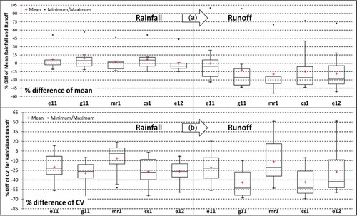
Using the five “best” downscaled GCMs, the error propagation ratios were found as follows: (a) mean difference: 1:−3; (b) standard deviation: 1:2; (c) normalized error: 1:3; and (d) normalized bias: 1:−2 (Table 5). These were the same ratios as obtained using all the downscaled GCMs. This implied that the use of many GCMs, to a large extent, cancels out inter-GCM variability, i.e. it cancels out any bias introduced by either overestimation or underestimation by the individual GCMs.

Table 5. Rainfall to runoff error propagation ratio for the mean, standard deviation (SD) and coefficient of variation (CV), normalized errors and normalized bias for all the WMAs in uMngeni catchment. NE: normalized error; NB: normalized bias.

WMA	Mean rainfall:runoff ratio	SD rainfall:runoff ratio	CV rainfall:runoff ratio	NE rainfall:runoff ratio	NB rainfall:runoff ratio
Mpendle	1:−1.91	1:0.67	1:0.44	1:2.13	1:−1.91
Lions River	1:−6.4	1:14	1:0.67	1:3	1:−6.4
Midmar	1:1.29	1:39.17	1:2.32	1:2.54	1:1.29
Karkloof	1:−1.55	1:4.17	1:0.69	1:2.48	1:−1.55
Albert Falls	1:−0.2	1:1.63	1:1.41	1:4.29	1:−0.2
Henley	1:1.93	1:0.54	1:1.08	1:2.36	1:1.93
Pietermaritzburg	1:3.18	1:5.5	1:8.83	1:3.67	1:3.18
New Hanover	1:5.17	1:4.67	1:−0.67	1:2.41	1:5.17
Nagle	1:−12.5	1:2.04	1:1.57	1:4.9	1:−12.5
Table Mountain	1:−1.14	1:2.6	1:3.92	1:3.13	1:−1.14
Mqeku	1:−3.43	1:2.39	1:1.33	1:3.58	1:−3.43
Inanda	1:−0.75	1:1.82	1:2.15	1:3.71	1:−0.75
Durban	1:−3.75	1:90	1:1.08	1:2.76	1:−3.75
uMngeni average	1:−3.4	1:2.6	1:1.59	1:3.58	1:−3.4

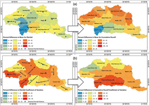
Of the five good GCMs, the GCM MIUB_ECHO_G (e11) was considered the best. Figure 7 shows the error propagation mapping for MIUB_ECHO_G (e11) in the uMngeni catchment, and Table 6 summarizes the error propagation from the different metrics for GCM e11. Using the best downscaled GCM, the error propagation of the mean rainfall to runoff was lower (1:−1) than when using all GCMs (1:−3). The same was also found with the NB ratio, which was also lower (1:−1) than when using all/best five GCMS (1:−2). This trend was attributed to the absence of extreme values of the selected GCM.

Table 6. MIUB_ECHO_G (e11): rainfall to runoff error propagation ratio for the mean, standard deviation (SD) and coefficient of variation (CV), normalized errors (NE) and normalized bias (NB) for all the WMAs in uMngeni catchment.

WMA	Mean rainfall:runoff ratio	SD rainfall:runoff ratio	CV rainfall:runoff ratio	NE rainfall:runoff ratio	NB rainfall:runoff ratio
Mpendle	1:−6	1:1	10:1	1:2	1:−6
Lions River	1:29	1:11	1:−2	1:3	1:29
Midmar	1:1	1:63	1:2	1:3	1:1
Karkloof	1:−3	1:4	5:1	1:3	1:−3
Albert Falls	3:1	1:1	1:1	1:5	3:1
Henley	1:2	6:1	1:1	1:2	1:2
Pietermaritzburg	1:3	1:−55	1:−3	1:3	1:3
New Hanover	1:3	1:1	1:−6	1:3	1:3
Nagle	1:−8	1:2	1:1	1:5	1:−8
Table Mountain	1:−2	1:7	1:−5	1:3	1:−2
Mqeku	6:1	1:1	1:1	1:4	22:1
Inanda	1:−2	1:1	1:2	1:4	1:−2
Durban	1:−1	1:−5	1:−1	1:3	1:−1
uMngeni average	1:−1	1:2	1:1	1:3	1:−1

Figure 7. Error propagation from rainfall to accumulated runoff: (a) mean rainfall to mean runoff, and (b) rainfall CV to accumulated runoff CV.

3.5 Error propagation for accumulated runoff

Of the 13 WMAs in uMngeni catchment, the following receive cumulated flows from their upstream sub-catchments: Midmar, Albert Falls, Pietermaritzburg, Nagle, Table Mountain, Inanda and Durban. Error propagation analysis was also carried out for these WMAs, the results of which are shown in Figure 6 and Table 7. Generally, catchment cumulative runoff showed an error propagation increase for the mean from 1:2 to 1:3, meaning that a 10% error in rainfall is tripled for total runoff as opposed to the doubling when considering runoff coming from the catchment only without upstream runoff contributions. There was a noted “dampening” of the error propagation for the percentage difference in mean rainfall and runoff for the Henley–Pietermaritzburg–Table Mountain catchments, with the upper catchment of Henley having a higher percentage difference as compared to downstream catchments of Table Mountain and Inanda (Fig. 7). However, this could not be said for all the other sub-catchments, as they exhibited no pattern at all.

Table 7. Error propagation summary results for (a) runoff from the catchment only and (b) accumulated runoff, for mean rainfall runoff, coefficient of variation, normalized error and normalized bias and the respective error propagation ratios.

(a)	dRF Mean	dRO Mean Catchment	dRO Mean Cumulative	dRO Mean Ratio Catchment	dRO Mean Ratio Cumulative	dCV RF	dCV RO Catchment	dCV RO Cumulative	CV Ratio Catchment	CV Ratio Cumulative
Midmar	34	44	−13	1:1	3:1	−28	−65	−23	1:2	1:1
Albert Falls	10	−2	−17	5:−1	1:−2	−39	−55	−25	1:1	1:1
Pietermaritzburg	−11	−35	20	1:3	1:−2	−6	−53	−63	1:9	1:10
Nagle	2	−25	−22	1:−12	1:−10	−30	−47	−25	1:2	1:1
Table Mountain	−7	8	8	1:−1	1:−1	−13	−51	−51	1:4	1:4
Inanda	−4	3	−15	1:−1	1:4	−20	−43	−25	1:2	1:1
Durban	4	−15	−14	1:−4	1:−4	−12	−13	−24	1:1	1:2
uMngeni average	4	−3	−8	1:−2	1:−3	−21	−47	−34	1:3	1:3
(b)	NE Rainfall	NE Runoff Catchment	NE Runoff Cumulative	NE Ratio Catchment	NE Ratio Cumulative	NB Rainfall	NB Runoff Catchment	NB Runoff Cumulative	NB Ratio Catchment	NB Ratio Cumulative
Midmar	0.4	1.0	0.5	1:3	1:1	0.34	0.44	−0.13	1:1	3:1
Albert Falls	0.2	0.9	0.5	1:4	1:2	0.10	−0.02	−0.17	5:1	1:−2
Pietermaritzburg	0.2	0.9	0.8	1:4	1:3	−0.11	−0.35	0.20	1:3	1:−2
Nagle	0.2	1.0	0.5	1:5	1:3	0.02	−0.25	−0.22	1:−12	1:−10
Table Mountain	0.2	0.7	0.7	1:3	1:3	−0.07	0.08	0.08	1:−1	1:−1
Inanda	0.3	1.0	0.5	1:4	1:2	−0.04	0.03	−0.15	1:−1	1:4
Durban	0.3	0.7	0.5	1:3	1:2	0.04	−0.15	−0.14	1:−4	1:−4
uMngeni average	0.3	0.9	0.6	1:4	1:3	0.04	−0.03	−0.08	1:−2	1:−3

Percentage differences (d): dRF Mean: of rainfall mean; dRO Mean Catchment: of mean rainfall to runoff from catchment only; dRO Mean Cumulative: of mean rainfall to runoff from all upstream catchments; dRO Mean Ratio Catchment: rainfall to runoff ratio for catchment only; dRO Mean Ratio Cumulative: rainfall:runoff ratio from all upstream catchments; dCV RF: of CV for rainfall; dCV RO Catchment: of CV for catchment runoff; dCV RO Cumulative: of CV for catchment plus upstream runoff; CV Ratio Catchment: CV ratio for catchment only; CV Ratio Cumulative: CV ratio for catchment plus upstream runoff.

NE: normalized error; NB: normalized bias; NE Rainfall: NE for rainfall; NE Runoff Catchment: NE for runoff from catchment; NE Runoff Cumulative: NE for cumulative runoff; NE Ratio catchment: ratio of NE for catchment rainfall to runoff; NE Ratio Cumulative: NE of rainfall to cumulative runoff ratio for catchment; NB Rainfall: normalized bias for rainfall; NB Runoff Catchment: NB for runoff from catchment; NB Runoff Cumulative: NB for cumulative runoff; NB Ratio catchment: NB for catchment rainfall to runoff ratio; NB Ratio Cumulative: NB for rainfall to cumulative runoff ratio for catchment.

Nevertheless, analysis of error propagation for variability within individual WMAs showed that runoff from the catchment only (minus upstream contribution) had more variability than the runoff inclusive of upstream runoff contribution, with error propagation being higher for Midmar, Nagle and Table Mountain (Table 7). Likewise, the mean bias was higher for runoff inclusive of upstream runoff contribution at 1:−3, as compared to 1:−2 for runoff from the catchment only. The mean error was higher for the runoff from the catchment only at 1:4, as compared to 1:3 for runoff inclusive of upstream runoff contribution.

4 Discussion and conclusions

As mentioned earlier, the hypothesis that there is no significant difference in errors between historical vs downscaled GCM rainfall and corresponding errors in simulated runoff from historical rainfall vs simulated runoff from GCM rainfall was tested herein. This study established that errors in rainfall were amplified in simulated runoff, and these were more amplified in the percentage difference of the mean (1:−3), as compared to the percentage difference of standard deviation (1:2). Likewise, the normalized errors and the normalized bias for rainfall showed a high error propagation ratio from rainfall to runoff of 1:3 and 1:−2, respectively. The error propagation could be attributed to several factors that can contribute to high runoff generation, such as antecedent soil moisture, storm duration, wet/dry sequences, number of rainy days, number of dry days, rainfall intensity, rain rates and frequency of extreme events, all of which still need to be satisfactorily represented during the downscaling process. Additionally, the noted extreme values (e.g. for Nagle), with a percentage difference of mean rainfall to runoff ratio of 1:−13, could be attributed to the influence of extreme/high values in the runoff simulation. The same could be said for Lions River and Midmar, which had a percentage difference of standard deviation from rainfall to runoff of 1:14 and 1:39, respectively. However, it was also noted that all of the WMAs had a negative bias in the percentage difference in standard deviation, which could be attributed to the influence of extreme values when using the standard deviation. It was concluded from the above that such error propagation leads to uncertainty propagation as well, when using GCM data to drive hydrological models.

The analysis presented here used metrics based on the mean and variance statistics only. These in most cases do not capture well the extreme values, hence will not capture well the occurrence of extreme events. Given the trends shown by the error propagation metrics above, it was concluded that, besides the mean and variance statistics, there is also a need to assess other rainfall characteristics, such as high and low rainfall, peak rainfall and their frequency, since according to Coutinho et al. (2014) these might be the rainfall features that influence runoff generation, in particular high and low rainfall events and their frequency of occurrence. Additionally, apart from rainfall amount, other aspects of rainfall also affect runoff generation, since runoff generation is driven not only by high rainfall events that last over several days, but also by preceding rainfall events that influence runoff by changing soil moisture content.

Previous studies established the importance of high and low rainfall runoff values, even though climate modelling was not necessarily under consideration. For example, results from a study by Teng et al. (2012) showed that the high runoff and low flows are not well captured using downscaled GCMs. Gabellani et al. (2007) also found that underestimating or predicting a lower value of the spectral slope of the rainfall field leads to a potential underestimation of the strength of peak discharge. Overall, it is important for the downscaled GCMs to better simulate the number and length of storms, and the dry periods that intersperse them (Vaze et al. 2010, Teng et al. 2012). Based on the results obtained, it is thus recommended to evaluate the performance of runoff simulated from downscaled GCM climate data in correctly capturing low flows and high flows. Ultimately, there is a need for continuous improvement in the GCM downscaling process, particularly model process description, so as to improve the downscaling process and minimize uncertainties due to GCM model description. Recent developments allude to a move towards this (see e.g. Chen et al. 2012, Liu et al. 2012, Li et al. 2013, Fand et al. 2014, Ji et al. 2014, 2014).

Analysis of the results from the different downscaled GCMs showed that CCMA_CGCM3_1 (cc1), CNRM_CM3 (cn1), CSIRO_MK3_5 (cs1), MPI_ECHAM5 (e12) and MRI_CGCM2_3_2A (mr1) had the lowest hydrological error propagation magnitude (Fig. 6). Of these, MPI_ECHAM5 (e12), CNRM_CM3 (cn1) and CSIRO_MK3_5 (cs1) had the lowest hydrological error propagation magnitude. Based on these results, it was concluded that these GCMs were better at capturing the full range of hydrological characteristics, including hydrological extremes, as well as the mean and variability. For these GCMs, the errors in simulated runoff show a similar pattern to those for downscaled rainfall, but are more magnified. It can therefore be concluded that these GCMs potentially provide quality input data and hence may be capturing other rainfall characteristics stated above, making them suitable for climate change hydrological impact analysis. Using several GCMs, as noted in this research, will give comparable results; however, it also has the potential of “hiding” inter-GCM variability.

In this study, two things therefore stand out as potential limitations: (a) the use of one rainfall station per WMA, and (b) the use of one hydrological model, hence the same process descriptions. It is therefore recommended to use several hydrological models as well as several rainfall stations within a specified catchment area for future studies, provided there are no limitations of data availability.

Concerning the use of a single hydrological model, from the results it was possible to infer that errors in the space–time description of rainfall are amplified in simulated runoff predictions, resulting in simulated runoff prediction uncertainty. This is also detailed by several other studies (e.g. Ogden et al. 2000, Senarath et al. 2000, Sharif et al. 2002, 2004). This could be attributed entirely to hydrological model development/model structure. Rainfall–runoff models typically route water through one or more conceptual storages. These one-dimensional stores represent two- or three-dimensional features of the catchment, and therefore the contents of conceptual stores are almost always spatially averaged. The observed forcing input is typically a spatial and temporal average of a random field, hence spatial and temporal averaging induces unavoidable errors in fluxes. This, in the output (runoff), is usually characterized by runs of systematic over- and underestimation, recessions are mis-specified, and peaks are spuriously simulated or completely missed (Beven and Binley 1992, Beven and Freer 2001, Pappenberger et al. 2005, Lumsden et al. 2009). Because the hydrological model may have interconnected stores, an error in one flux can propagate through “downstream” stores and thus affect other fluxes. This induces a persistent error in the fluxes dependent on the downstream store.

Regarding the use of a single (at most two) rainfall station(s) with sufficient records to represent a single WMA, the WMAs were of different sizes, with the largest (Nagle, 454 km²) being almost twice as large as the smallest (Mqeku, 244 km²), a difference of 54%. As a result, the higher hydrological propagation errors could have been due partly to the larger catchment surface areas being represented by one rain station (i.e. under representation). Such limitations of data availability are characteristic of southern Africa and elsewhere, as previously highlighted by Kusangaya et al. (2014), Nikulin et al. (2012) and Mazvimavi (2010).

Acknowledgements

We would like to thank the Climate System Analysis Group at the University of Cape Town for providing the downscaled rainfall data.

Disclosure statement

No potential conflict of interest was reported by the authors.

Additional information

Funding

We would like to thank the Applied Centre for Climate and Earth Systems Science (ACCESS) for supporting this research work by providing funds for undertaking the PhD research under the theme “Climate Change Impacts and Adaptation”.

References

- Acocks, J.P.H., 1988. Veld types of South Africa. 3rd ed. Pretoria: Government Printers.
- Andréassian, V., et al. 2001. Impact of imperfect rainfall knowledge on the efficiency and the parameters of watershed models. Journal of Hydrology, 250 (1–4), 206–223. doi:10.1016/S0022-1694(01)00437-1
- Arnell, N.W. and Gosling, S.N., 2013, The impacts of climate change on river flow regimes at the global scale. Journal of Hydrology, 486 (1), 351–364. doi:10.1016/j.jhydrol.2013.02.010
- Beven, K. and Binley, A., 1992. The future of distributed models: model calibration and uncertainty prediction. In: B. E Moore, ed. Terrain analiysis and distributed modelling in hydrology. Chichester: John Wiley & Sons, 227–246.
- Beven, K. and Freer, J., 2001, Equifinality, data assimilation, and uncertainty estimation in mechanistic modelling of complex environmental systems using the GLUE methodology. Journal of Hydrology, 249 (1–4), 11–29. doi:10.1016/S0022-1694(01)00421-8
- Beven, K.J., 2011. Rainfall-runoff modelling: the primer. Chichester: John Wiley & Sons.
- Bezuidenhout, C.N., 2005. Development and evaluation of model-based operational yield forecasts in the South African sugar industry. ( PhD). University of KwaZulu-Natal, South Africa.
- Borga, M., 2002, Accuracy of radar rainfall estimates for streamflow simulation. Journal of Hydrology, 267 (1–2), 26–39. doi:10.1016/S0022-1694(02)00137-3
- Borga, M., Degli Esposti, S., and Norbiato, D., 2006. Influence of errors in radar rainfall estimates on hydrological modeling prediction uncertainty. Water Resources Research, 42 (8). doi:10.1029/2005WR004559
- Bringi, V., et al. 2001. An areal rainfall estimator using differential propagation phase: evaluation using a C-band radar and a dense gauge network in the tropics. Journal of Atmospheric and Oceanic Technology, 18 (11), 1810–1818. doi:10.1175/1520-0426(2001)018<1810:AAREUD>2.0.CO;2
- Chen, H., Xu, C.-Y., and Guo, S., 2012, Comparison and evaluation of multiple GCMs, statistical downscaling and hydrological models in the study of climate change impacts on runoff. Journal of Hydrology, 434–435 (0), 36–45. doi:10.1016/j.jhydrol.2012.02.040
- Chiew, F., et al. 2010. Comparison of runoff modelled using rainfall from different downscaling methods for historical and future climates. Journal of Hydrology, 387 (1–2), 10–23. doi:10.1016/j.jhydrol.2010.03.025
- Coutinho, J., et al., 2014. Characterization of sub-daily rainfall properties in three raingauges located in northeast Brazil. Proceedings of the International Association of Hydrological Sciences, 364, 345–350. doi:10.5194/piahs-364-345-2014
- Fand, B.B., et al. 2014. Predicting the impact of climate change on regional and seasonal abundance of the mealybug Phenacoccus solenopsis Tinsley (Hemiptera: pseudococcidae) using temperature-driven phenology model linked to GIS. Ecological Modelling, 288 (0), 62–78. doi:10.1016/j.ecolmodel.2014.05.018
- Gabellani, S., et al. 2007. Propagation of uncertainty from rainfall to runoff: A case study with a stochastic rainfall generator. Advances in Water Resources, 30 (10), 2061–2071. doi:10.1016/j.advwatres.2006.11.015
- Gorard, S., 2005, Revisiting a 90-year-old debate: the advantages of the mean deviation. British Journal of Educational Studies, 53 (4), 417–430. doi:10.1111/j.1467-8527.2005.00304.x
- Gosling, S., et al. 2011. A comparative analysis of projected impacts of climate change on river runoff from global and catchment-scale hydrological models. Hydrology and Earth System Sciences, 15 (1), 279–294. doi:10.5194/hess-15-279-2011
- Graham, L.P., et al. 2011. Using multiple climate projections for assessing hydrological response to climate change in the Thukela River Basin, South Africa. Physics and Chemistry of the Earth, Parts A/B/C, 36 (14–15), 727–735. doi:10.1016/j.pce.2011.07.084
- Gush, M., et al. 2002. A new approach to modelling streamflow reductions resulting from commercial afforestation in South Africa. The Southern African Forestry Journal, 196 (1), 27–36. doi:10.1080/20702620.2002.10434615
- Hargreaves, G.H. and Samani, Z.A., 1985, Reference crop evapotranspiration from temperature. Applied Engineering in Agriculture, 1 (2), 96–99. doi:10.13031/2013.26773
- Hewitson, B. and Crane, R., 2006, Consensus between GCM climate change projections with empirical downscaling: precipitation downscaling over South Africa. International Journal of Climatology, 26 (10), 1315–1337. doi:10.1002/(ISSN)1097-0088
- Hewitson, B.C., and Tadross, M.A., 2011. Developing regional climate change projections. In: R.E. Schulze, B.C. Hewitson, K.R. Barichievy, M.A. Tadross, R.P. Kunz, M.J.C. Horan, T.G. Lumsden, eds. Methodological approaches to assessing eco-hydrological responses to climate change in South Africa. Report K5/1562. Pretoria: Water Research Commission.
- Honti, M., Scheidegger, A., and Stamm, C., 2014, The importance of hydrological uncertainty assessment methods in climate change impact studies. Hydrology and Earth System Sciences, 18 (8), 3301–3317. doi:10.5194/hess-18-3301-2014
- Hossain, F., et al. 2004. Hydrological model sensitivity to parameter and radar rainfall estimation uncertainty. Hydrological Processes, 18 (17), 3277–3291. doi:10.1002/hyp.5659
- Hostache, R., et al. 2011. Propagation of uncertainties in coupled hydro-meteorological forecasting systems: A stochastic approach for the assessment of the total predictive uncertainty. Atmospheric Research, 100 (2–3), 263–274. doi:10.1016/j.atmosres.2010.09.014
- Hughes, D., 2004, Three decades of hydrological modelling research in South Africa. South African Journal of Science, 100 (11 & 12), 638–642.
- Hughes, D., 2013. A review of 40 years of hydrological science and practice in southern Africa using the Pitman rainfall-runoff model. Journal of Hydrology, 501, 111–124. doi:10.1016/j.jhydrol.2013.07.043
- Hughes, D., 2016. Hydrological modelling, process understanding and uncertainty in a southern African context: lessons from the northern hemisphere. Hydrological Processes, 30 (14), 2419–2431. doi:10.1029/2008WR006833
- Hughes, D., Kapangaziwiri, E., and Sawunyama, T., 2010, Hydrological model uncertainty assessment in southern Africa. Journal of Hydrology, 387 (3–4), 221–232. doi:10.1016/j.jhydrol.2010.04.010
- Hughes, D., Mantel, S., and Mohobane, T., 2014, An assessment of the skill of downscaled GCM outputs in simulating historical patterns of rainfall variability in South Africa. Hydrology Research, 45 (1), 134–147. doi:10.2166/nh.2013.027
- Ji, F., et al. 2014. Evaluating rainfall patterns using physics scheme ensembles from a regional atmospheric model. Theoretical and Applied Climatology, 115 (1–2), 297–304. doi:10.1007/s00704-013-0904-2
- Kapangaziwiri, E., Hughes, D., and Wagener, T., 2012, Incorporating uncertainty in hydrological predictions for gauged and ungauged basins in southern Africa. Hydrological Sciences Journal, 57 (5), 1000–1019. doi:10.1080/02626667.2012.690881
- Kienzle, S.W., et al. 2012. Simulating the hydrological impacts of climate change in the upper North Saskatchewan River basin, Alberta, Canada. Journal of Hydrology, 412–413 (0), 76–89. doi:10.1016/j.jhydrol.2011.01.058
- Kusangaya, S., et al., 2014. Impacts of climate change on water resources in southern Africa: A review. Physics and Chemistry of the Earth, Parts A/B/C, 67, 47–54. doi:10.1016/j.pce.2013.09.014
- Kusangaya, S., et al., 2016. An evaluation of how downscaled climate data represents historical precipitation characteristics beyond the means and variances. Global and Planetary Change, 144, 129–141. doi:10.1016/j.gloplacha.2016.07.014
- Li, F., et al. 2013. The impact of climate change on runoff in the southeastern Tibetan Plateau. Journal of Hydrology, 505 (0), 188–201. doi:10.1016/j.jhydrol.2013.09.052
- Li, F., Zhang, G., and Xu, Y.J., 2014, Spatiotemporal variability of climate and streamflow in the Songhua River Basin, northeast China. Journal of Hydrology, 514 (0), 53–64. doi:10.1016/j.jhydrol.2014.04.010
- Liu, Y., et al. 2012. Quantifying uncertainty in catchment-scale runoff modeling under climate change (case of the Huaihe River, China). Quaternary International, 282 (0), 130–136. doi:10.1016/j.quaint.2012.04.029
- Liu, Y. and Gupta, H.V., 2007, Uncertainty in hydrologic modeling: toward an integrated data assimilation framework. Water Resources Research, 43 (7), W07401. doi:10.1029/2006WR005756
- Lumsden, T., Schulze, R., and Hewitson, B., 2009, Evaluation of potential changes in hydrologically relevant statistics of rainfall in Southern Africa under conditions of climate change. Water Sa, 35 (5), 649–656. doi:10.4314/wsa.v35i5.49190
- Mazvimavi, D., 2010, Climate change, water availability and supply. SARUA Leadership Dialogue Series, 2 (4), 81–97.
- Moulin, L., Gaume, E., and Obled, C., 2009, Uncertainties on mean areal precipitation: assessment and impact on streamflow simulations. Hydrology and Earth System Sciences, 5 (4), 2067–2110. doi:10.5194/hessd-5-2067-2008
- Najafi, M., Moradkhani, H., and Jung, I., 2011, Assessing the uncertainties of hydrologic model selection in climate change impact studies. Hydrological Processes, 25 (18), 2814–2826. doi:10.1002/hyp.v25.18
- Nikolopoulos, E.I., et al. 2010. Understanding the scale relationships of uncertainty propagation of satellite rainfall through a distributed hydrologic model. Journal of Hydrometeorology, 11 (2), 520–532. doi:10.1175/2009JHM1169.1
- Nikulin, G., et al. 2012. Precipitation climatology in an ensemble of CORDEX-Africa regional climate simulations. Journal of Climate, 25 (18), 6057–6078. doi:10.1175/JCLI-D-11-00375.1
- NWA, 1998. National Water Act, Act No. 36 of 1998. Pretoria, RSA: Government Printers.
- Ogden, F., et al. 2000. Hydrologic analysis of the Fort Collins, Colorado, flash flood of 1997. Journal of Hydrology, 228 (1–2), 82–100. doi:10.1016/S0022-1694(00)00146-3
- Pappenberger, F., et al. 2005. Cascading model uncertainty from medium range weather forecasts (10 days) through a rainfall-runoff model to flood inundation predictions within the European Flood Forecasting System (EFFS). Hydrology and Earth System Sciences Discussions, 9 (4), 381–393. doi:10.5194/hess-9-381-2005
- Praskievicz, S. and Chang, H., 2009, A review of hydrological modelling of basin-scale climate change and urban development impacts. Progress in Physical Geography, 33 (5), 650–671. doi:10.1177/0309133309348098
- Sawunyama, T. and Hughes, D., 2008, Application of satellite-derived rainfall estimates to extend water resource simulation modelling in South Africa. Water Sa, 34 (1), 1–10.
- Schulze, R., 1995. Hydrology and agrohydrology: A text to accompany the ACRU 3.00 agrohydrological modelling system. Pretoria, South Africa: Water Research Commission.
- Schulze, R., 2005. Climate change and water resources in Southern Africa: studies on scenarios, impacts, vulnerabilities and adaptation. Pretoria, South Africa: Water Research Commission.
- Schulze, R., 2011. Methodological approaches to assessing eco-hydrological responses to climate change in South Africa. Pretoria, South Africa: Water Research Commission.
- Schulze, R., Kunz, R., and Knoesen, D., 2003. Atlas of climate change and water resources in South Africa. Pretoria, South Africa: Water Research Commission.
- Schulze, R. and Maharaj, M., 2004. Development of a database of gridded daily temperatures for Southern Africa. Pretoria, South Africa: Water Research Commission.
- Schulze, R., and Perks, L., 2000. Assessment of the impact of climate change on hydrology and water resources in South Africa. ACRUcons Report 33. Pretoria: Water Research Commission.
- Senarath, S.U., et al. 2000. On the calibration and verification of two‐dimensional, distributed, Hortonian, continuous watershed models. Water Resources Research, 36 (6), 1495–1510. doi:10.1029/2000WR900039
- Sharif, H.O., et al. 2002. Numerical simulations of radar rainfall error propagation. Water Resources Research, 38 (8). doi:10.1029/2001WR000525
- Sharif, H.O., et al. 2004. Statistical analysis of radar rainfall error propagation. Journal of Hydrometeorology, 5 (1), 199–212. doi:10.1175/1525-7541(2004)005<0199:SAORRE>2.0.CO;2
- Smithers, J. and Schulze, R., 1995. ACRU Agrohydrological Modelling System: User manual, version 3.00. (Report TT70/95). Pretoria: Water Research Commission.
- Smithers, J., Schulze, R., and Kienzle, S., 1997, Design flood estimation using a modelling approach: a case study using the ACRU model. IAHS Publications-Series of Proceedings and Reports-Intern Assoc Hydrological Sciences, 240, 365–376.
- Summerton, M., 2008. A preliminary assessment of the impact of climate change on the water resources of the uMgeni catchment. Report Number 160.8/R001/2008. Pietermaritzburg: Umgeni Water, Planning Services Department.
- Summerton, M., and Schulze, R., 2009. A framework for determining the possible impacts of a changing climate on water supply. In: Starrett, S. eds. World environmental and water resources congress 2009@ great rivers, 2012, Kansas City, MO, 4623–4633.
- Summerton, M., Schulze, R., and Graham, P., 2010. Impacts of a changing climate on hydrology and water supply in the Mgeni catchment, South Africa. In: Walsh, C. eds. Proceedings of the British hydrological society third international symposium, managing consequences of a changing global environment, Newcastle UK.
- Summerton, M., Schulze, R., and Liebscher, H., 2009, Hydrological consequences of a changing climate: the Umgeni Water utility case study. IAHS Publication, 327, 237.
- Tadross, M., Jack, C., and Hewitson, B., 2005, On RCM‐based projections of change in southern African summer climate. Geophysical Research Letters, 32 (23), 23–35. doi:10.1029/2005GL024460
- Tarboton, K. and Schulze, R., 1992. Distributed hydrological modelling system for the mgeni catchment. Pretoria, South Africa: Water Research Commission.
- Teng, J., et al. 2012. Assessment of an analogue downscaling method for modelling climate change impacts on runoff. Journal of Hydrology, 472–473 (0), 111–125. doi:10.1016/j.jhydrol.2012.09.024
- Vaze, J., et al. 2010. Climate non-stationarity–validity of calibrated rainfall–runoff models for use in climate change studies. Journal of Hydrology, 394 (3–4), 447–457. doi:10.1016/j.jhydrol.2010.09.018
- Warburton, M., Schulze, R., and Jewitt, G., 2010, Confirmation of ACRU model results for applications in land use and climate change studies. Hydrology and Earth System Sciences, 14 (12), 2399–2414. doi:10.5194/hess-14-2399-2010
- Warburton, M., Schulze, R., and Maharaj, M., 2005. Is South Africa’s temperature changing? An analysis of trends from daily records, 1950–2000. In: Schulze, R. eds. Climate change and water resources in southern Africa: studies on scenarios, impacts, vulnerabilities and adaptation (WRC Report 1430/1/05). Pretoria: Water Research Commission, 275–295.
- Warburton, M.L., Schulze, R.E., and Jewitt, G.P., 2012. Hydrological impacts of land use change in three diverse South African catchments. Journal of Hydrology, 414, 118–135. doi:10.1016/j.jhydrol.2011.10.028
- Zhang, X., Xu, Y.-P., and Fu, G., 2014, Uncertainties in SWAT extreme flow simulation under climate change. Journal of Hydrology, 515 (0), 205–222. doi:10.1016/j.jhydrol.2014.04.064
- Zhijia, L., et al., 2004. Coupling between weather radar rainfall data and a distributed hydrological model for real-time flood forecasting. Hydrological Sciences Journal, 49 (6), 945–958.
- Zhu, D., Peng, D., and Cluckie, I., 2013, Statistical analysis of error propagation from radar rainfall to hydrological models. Hydrology and Earth System Sciences, 17 (4), 1445–1453. doi:10.5194/hess-17-1445-2013