On the prediction of persistent processes using the output of deterministic models

ABSTRACT

A problem frequently met in engineering hydrology is the forecasting of hydrological variables conditional on their historical observations and the hindcasts and forecasts of a deterministic model. On the contrary, it is a common practice for climatologists to use the output of general circulation models (GCMs) for the prediction of climatic variables despite their inability to quantify the uncertainty of the predictions. Here we apply the well-established Bayesian processor of forecasts (BPF) for forecasting hydroclimatic variables using stochastic models through coupling them with GCMs. We extend the BPF to cases where long-term persistence appears, using the Hurst-Kolmogorov process (HKp, also known as fractional Gaussian noise) and we investigate its properties analytically. We apply the framework to calculate the distributions of the mean annual temperature and precipitation stochastic processes for the time period 2016–2100 in the United States of America conditional on historical observations and the respective output of GCMs.

KEYWORDS:

• Bayesian processor of forecasts
• fractional Gaussian noise
• general circulation model
• Hurst-Kolmogorov
• hydroclimatic prediction
• hydrological statistics

Editor A. Castellarin; Associate editor A. Viglione

1 Introduction

1.1 Uncertainty in deterministic models in hydrological science

Recently, various studies regarding the prediction of hydrological variables based on stochastic models have been published. To mention some of them, Koutsoyiannis et al. (2008b) proposed a stochastic model for the prediction of the Nile flow a month ahead. On longer time scales, Koutsoyiannis et al. (2007) proposed a stochastic framework to calculate future climatic uncertainties conditional on historical observations, while Tyralis and Koutsoyiannis (2014) solved this problem using a Bayesian framework. Engineering hydrologists frequently use stochastic models for the prediction of hydrological variables, whereas the climatologists focus on deterministic models (general circulation models, GCMs) (Koutsoyiannis et al. 2008a). While it is true that deterministic models incorporate knowledge of the climatic mechanisms expressed through deterministic equations, they are not appropriate to quantify the uncertainty of predictions. Consequently, climatologists have recently started reconsidering their approach, introducing stochastic models in climate science (Macilwain 2014), while earlier Schneider (2002) set a debate on how and when to assign probabilities to future projections of the GCMs, simultaneously expressing some concerns about their absence in specific cases.

Estimating uncertainties of forecasted geophysical variables using information from deterministic models is frequently met in hydrological science and, in particular, in rainfall–runoff modelling (e.g. Montanari and Grossi 2008, Wang et al. 2009, Zhao et al. 2011, Smith et al. 2012, Pokhrel et al. 2013, Zhao et al. 2015a). The Bayesian forecasting system (BFS) and its extensions in a series of papers (Krzysztofowicz 1999b, 2001, 2002, Krzysztofowicz and Maranzano 2004) is a primary tool for estimating uncertainties in rainfall–runoff modelling. Another interesting tool for quantifying uncertainties is the Bayesian processor of forecasts (BPF) introduced in Krzysztofowicz (1985) and compared with the BFS in Krzysztofowicz (1999a). The BPF “combines a prior distribution, which describes the natural uncertainty about the realization of a hydrologic process, with a likelihood function, which describes the uncertainty in categorical forecasts of that process, and outputs a posterior distribution of the process, conditional upon the forecasts” (Krzysztofowicz 1985). It is mostly used for weather forecasting and, while it is a general algorithm that can be applied to any distribution and dependence pattern of the process, it has been investigated solely for independent or Markov-dependent variables (e.g. Krzysztofowicz 1999a, Krzysztofowicz and Evans 2008, Chen et al. 2013). The term “Bayesian” refers to the use of the Bayes theorem; however, the BPF does not use full Bayesian statistics. Consequently, the parameter uncertainty (Montanari and Koutsoyiannis 2012) is not considered in the model.

A frequent approach for modelling mean annual geophysical time series is the implementation of the Hurst-Kolmogorov stochastic process (HKp) (also known as fractional Gaussian noise, e.g. Koutsoyiannis 2002, 2003, 2006b, Koutsoyiannis and Montanari 2007). The investigation of big geophysical datasets has confirmed the HK behaviour of geophysical variables on the annual time scale (Fatichi et al. 2012, Iliopoulou et al. 2016, Markonis and Koutsoyiannis 2016). The HK process is suitable for modelling the variability observed in geophysical time series, and not only because it can model the HK behaviour. Specifically, while it is stationary (for the benefits of using stationary models see Koutsoyiannis and Montanari 2014, Montanari and Koutsoyiannis 2014), it can model higher variations of the observed time series, unlike the Markovian models. Thus, it can model observed trends (Koutsoyiannis 2006a) and it does not underestimate uncertainties of the forecasted variable (Tyralis and Koutsoyiannis 2014).

1.2 General circulation models

The Coupled Model Intercomparison Project Phase 5 (CMIP5) includes GCMs, which contain historical runs, i.e. simulations of the past forced by observed atmospheric composition changes and time-evolving land cover (Taylor et al. 2012). Each historical run is extended with a projection of the climate driven by concentration or emission scenarios consistent with the representative concentration scenarios (RCPs; Hibbard et al. 2007, Moss et al. 2010). The evaluation of GCMs for reproducing the past has been studied extensively with varying results, depending on the examined variable (usually temperature and precipitation), time scale of the variable, statistic or parameter of interest, region and time period. Most studies include comparisons with observations, re-analysis data, satellite data or all such data (Koutsoyiannis et al. 2008a, Anagnostopoulos et al. 2010, Santer et al. 2013, Xu et al. 2013, Sheffield et al. 2013a, 2013b, Koutroulis et al. 2015, Nasrollahi et al. 2015, Aloysius et al. 2016, Matthes et al. 2016), visualizations (Potter et al. 2009) and even comparisons between the models themselves (Johnson and Sharma 2009). However, Notz (2015) points out that the direct comparison of model simulations with observations allows for limited inferences about the deficiencies of the model.

Of practical interest and gaining place in the literature is the quantification of the uncertainties of the GCM projections (Katz 2002), whose sources are measurement errors, variations of the geophysical processes and model structure, according to Katz (2002), or internal variability, scenario and model uncertainties (e.g. Hawkins and Sutton 2009). Therefore, it is apparent that we cannot consider raw projections as a product that we can use without further processing. A significant part of the literature has been devoted to the quantification of the uncertainties (Hawkins et al. 2014, Woldemeskel et al. 2014, Tian et al. 2015, Zhao et al. 2015b) and their partition (Hawkins and Sutton 2009, 2011, Yip et al. 2011, Ylhäisi et al. 2015, Hewitt et al. 2016), usually to internal, scenario and model uncertainties. Beyond what narrowly concerns climate science, there is a discussion on the uncertainty attributed to human behaviour, which seems not quantifiable. Consequently, the use of scenarios is proposed (Dessai and Hulme 2004) to consider human behaviour with the use of RCPs. There is also a discussion on the potential of the reduction of uncertainties (Hawkins and Sutton 2009, 2011), while Knutti and Sedláček (2013) conclude that progress in terms of narrowing uncertainties is too limited. An overview of methods to evaluate the uncertainty of deterministic models, not only in the climate science, is presented in Uusitalo et al. (2015).

The limitations in reducing uncertainties are primarily due to the internal climate variability (Knutti and Sedláček 2013); thus, the development of methods that are based on GCMs and simulate the local weather (e.g. Groves et al. 2008) gains a place in practical applications of the GCMs. While future climate is still projected based on single GCM outputs (Maloney et al. 2014), combining multiple models for future projections is proposed as an alternative for skilful climate predictions (Smith et al. 2009, Chowdhury and Sharma 2011, Strobach and Bel 2015). However, Pirtle et al. (2010) claim that the quality of analyses based on multiple models cannot be evaluated, while Kundzewicz and Stakhiv (2010) mention that the spread of outcomes of the GCMs is incorrectly used as a type of uncertainty analysis. The so-called “bias corrections” refer to another group of methods that are used to improve the projections of GCMs through (a posteriori) increasing the agreement between GCM outputs and observations. However, this procedure is artificial and is criticized for hiding the uncertainty rather than reducing it (Ehret et al. 2012).

1.3 On the proposed framework

It seems that the arsenal of methods to improve the GCM projections and quantify their forecasting uncertainty (mainly use of multiple models and “bias correction”) is inadequate. In the present study, we propose using the BPF, which is based on a solid scientific foundation, i.e. the concept of conditional stochastic independence (de Finetti 1974, Krzysztofowicz 1985). Hence, it can be an appropriate alternative. Here we apply the BPF to quantify the uncertainties in the forecasts of mean annual temperature and precipitation. We model the variables of interest with the HKp, which we assume is the prior distribution that describes the natural uncertainty about the realization of the process. The deterministic forecasts of the process are the GCM outputs, while the BPF outputs the posterior distribution of the process conditional on the GCM outputs and the realization of the process.

The posterior distribution depends initially on the fitted HKp, but eventually (and in a determinative manner) on the agreement of the GCM output with the observations. The model uses six parameters. The three parameters of the HKp are estimated from the observations. The degree of agreement of the GCM with the observations is determined by three parameters, estimated when fitting the model using a common period of observations and GCM output. The two fittings are performed independently. As a result, application of the BPF avoids artificial improvement of the model (e.g. “bias correction” and related methods), while the natural variability of the process is modelled using a well-established stochastic model. Furthermore, uncertainties are quantified using a single output of the model, while the human influence is modelled through the selection of a single scenario. Finally, we avoid narrowing uncertainty. Instead, uncertainties are presented as they are, i.e. without reducing them artificially.

The theoretical contribution of the present study is the application of the BPF to processes with more complicated dependence structure compared to the Markovian model. We apply the BPF to the HKp, which results in posterior multivariate normal distributions. We apply the framework to the mean annual temperature and total annual precipitation in a large area, the contiguous part of the United States of America, while we show whether and how a purely probabilistic forecast could be improved by using a deterministic forecast.

2 Methods

In this section, we present the BPF, the definition of the HKp, and the application of the BPF to normal stationary stochastic processes and as a case study to the HKp. In the next sections we use the Dutch convention for notation, according to which random variables and stochastic processes are underlined (Hemelrijk 1966).

2.1 The Bayesian processor of forecasts

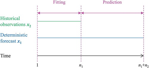
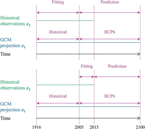
Let x_2(1:(n1+n2)) be a geophysical process that we wish to forecast and x_1(1:(n1+n2)) be its forecast given by a deterministic model. The respective time periods (in discrete time, denoted through the integers n₁ and n₂) for each variable are presented in Figure 1. We assume that x_2(1:n1) denotes the observed (historical) values of the time series, while x_1(1:(n1+n2)) and x_2(1:(n1+n2)) are the stochastic processes that represent in stochastic terms the deterministic model and the geophysical process, respectively, defined in Equations (1) and (2) :

(1)

(2)

Figure 1. Time periods for the BPF data input and output. The prediction time period refers to the distribution of y₄|y₃, x₁. y₃ and y₄ are defined in Equations (7) and (8).

To shorten the equations used in the subsequent sections we use the notation of Equations (3)–(8), in which we remove the time indexes:

(3)

(4)

(5)

(6)

(7)

(8)

Henceforth, y₁ will be called the deterministic hindcast. The BPF is based on the fundamental Equations (9) and (10), which exploit the concept of conditional stochastic independence (for intuitive explanations of the BPF the reader is referred to de Finetti 1974, Krzysztofowicz 1985):

(9)

(10)

The deterministic forecasts are independent of each other conditional on the observations according to Equation (9) (Krzysztofowicz 1985), while each forecast depends only on the parallel observation according to Equation (10). Equations (9) and (10) combined result in:

(11)

Given an observation of x₂, the distribution of x₁ is determined by Equations (9) and (10). The purpose of the BPF is to find the distribution of y₄ conditional on y₃ and x₁, which is given by:

(12)

where both g() and ξ() denote (joint) distributions (more precisely, probability densities).

As proved in Appendix 1, h can be simulated using the equation:

(13)

Consequently, to simulate from h we must calculate the distributions f and g.

2.2 Α normal stationary stochastic process in the Bayesian processor of forecasts

Let x₂ denote a normal stationary stochastic process (Wei 2006, p. 10) with parameters μ, σ, ρ_i,j, given by:

(14)

(15)

(16)

The joint distribution of x₂ is multivariate normal with constant mean μ and autocovariance matrix Σ given by Equation (17). Furthermore, the joint distributions of y₃, y₄ and all subsets of x₂ are also multivariate normal, with the same mean and autocovariance matrix given by extracting respective parts of Σ. The proofs of the results of Section 2.2 are given in Appendix 1.

(17)

The autocovariance matrix Σ can be partitioned in the following way:

(18)

where the dimensions of the matrices are: R₁₁: n₁×n₁, R₂₁: n₂×n₁, R₁₂: n₁×n₂, R₂₂: n₂×n₂. Then the distribution of y₄|y₃ is given by:

(19)

where N denotes the multivariate normal distribution and:

(20)

(21)

(22)

(23)

An intuitive modelling of the relationship between x_1n and x_2n is given by the distribution (24) (e.g. Krzysztofowicz 1999a):

(24)

where:

(25)

Equation (24) means that the deterministic forecast x_1n can be modelled as a linear function of the observation x_2n. Thus, the level of the deterministic forecast depends on the level of the observation, while its variation is modelled by a constant parameter, regardless of the level of x_2n. Given Equations (9), (10) and (24), we prove in Appendix 1 that the distribution of y₄ conditional on y₂ is:

(26)

where

(27)

(28)

(29)

Combining Equations (19) and (26), we prove in Appendix 1 that the joint distribution of the future process of interest, given the historical observations and the deterministic forecast, is:

(30)

where:

(31)

(32)

2.3 Estimation of the parameters of the Bayesian processor of forecasts

The parameters of the BPF are μ, σ, ρ_|i−j| defined in Equations (14)–(16) and a, b, σ²_e defined in Equations (24) and (25). The parameters μ, σ, ρ_|i−j| can be estimated from fitting the joint distribution of y₃ to y₃. In the next sections, we will use the maximum likelihood estimator. The parameters a, b, σ_e can be estimated from the linear regression of x_1n on x_2n over the time period {1, …, n₁}. Figure 1 depicts the fitting periods.

2.4 Distinct fitting periods and other special cases

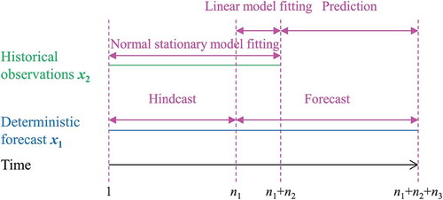
Sometimes the periods of fitting of the normal stationary model to estimate the parameters and fitting of the linear model to estimate the parameters a, b, σ_e do not coincide. In such cases, the parameters can be estimated in distinct periods. For example, in Figure 2, we assume that the deterministic model has already used information from the historical observations to adjust the hindcast, therefore the period cannot be used for the linear model fitting. However, the period of observations can be used for fitting the normal stationary model. In such cases, the intersection of the deterministic forecast period and the historical observations can be used for fitting the linear model. We present the distributions of interest and the proofs in Appendix 2.

Figure 2. Time periods for the BPF data input and output and the related periods for model fitting in the case of distinct periods.

In cases where the geophysical process is non-negative (e.g. precipitation), the modelling framework should be adapted to truncated variables. The necessity for doing this appears when the coefficient of variation of the process is high (so that the probability of getting a negative value from the normal distribution is not negligible). For such cases, the BPF can be extended to include truncated normal distributions (Horrace 2005).

2.5 Hurst-Kolmogorov process

The model of interest for x₂ is the HKp, as explained in Section 1.1. The HKp is a three-parameter normal stationary stochastic process in discrete time. Its parameters μ and σ are defined by Equations (14) and (15), while its parameter H is defined by Equation (33) (Tyralis and Koutsoyiannis 2011):

(33)

We use the maximum likelihood estimator to estimate μ, σ and H simultaneously, as proposed in Tyralis and Koutsoyiannis (2011), while the estimator is implemented in the R package HKprocess (Tyralis 2016).

2.6 Investigation for various values of the parameters of the Bayesian processor of forecasts

For specific values of the parameters of the BPF and, in particular, of the linear model, we can understand its behaviour in extreme cases. We present the proofs of the results of Section 2.6 in Appendix 3. A similar investigation is presented in Krzysztofowicz (1985).

If σ_e = 0, i.e. the deterministic model is perfect, then the BPF forecast prediction interval is 0, while the BPF forecast is equal to the deterministic forecast (see Equations (C.4) and (C.5)). When a = 0 (see Equation (25)), then the deterministic forecast does not improve the BPF forecast. Then the BPF forecast is equal to the forecast of the stochastic process (see Equation (C.8)). This problem has already been solved in Tyralis and Koutsoyiannis (2014), who also employed a Bayesian treatment of the parameters of the stochastic process. Intuitively, high values of σ_e will result in high uncertainties. Furthermore, negative values of a will result in BPF forecasts with inverse trends compared to the deterministic forecasts.

We can also assess the quality of the deterministic model using the sufficiency characteristic defined in Krzysztofowicz (1987) and the informativeness score defined in Krzysztofowicz (1992, 2010). The sufficiency characteristic (SC) and the informativeness score (IS), defined respectively by Equations (34) and (35), summarize the information contained in the parameters a and σ:

(34)

(35)

Krzysztofowicz (2010) proved that:

(36)

where r is Pearson’s r defined by:

(37)

For an intuitive explanation of the SC and the IS the reader is referred to Krzysztofowicz (2010). In brief, the SC is interpretable as a “signal-to-noise ratio”, with |a| being the measure of the signal, and σ being the measure of the noise, while the posterior variance depends on the SC. The SC ranges in the interval [0, ∞] and the IS ranges in the interval [0, 1]. Higher values of both parameters imply a more informative deterministic model and lower posterior variance. For the perfect deterministic model we have SC = ∞ and IS = 1, while for a completely uninformative deterministic model we have SC = 0 and IS = 0.

Normal stationary stochastic processes have finite first and second order moments, therefore μ and σ defined in Equations (14) and (15) are finite. Subsequently, the results presented in Appendix 3 can be generalized using the SC and IS parameters. For instance, a = 0 implies SC = 0 and IS = 0, while implies SC = 1 and IS = ∞. Furthermore, the SC and the IS can be estimated from different samples, e.g. as in Figure 2. In such case |r| ≠ IS (Krzysztofowicz 2010), and both parameters provide different information. Further investigations using simulations for special (artificially designed) cases will be presented in Section 4.1.

3 Data

We apply the BPF to instrumental temperature and precipitation data, which we aggregated on the annual time scale, and to the GCM projections, which we used as deterministic forecasts.

3.1 Temperature data

We use monthly temperature data from the unadjusted version 3 of the Global Historical Climatology Network-Monthly (GHCN-M) temperature dataset (Lawrimore et al. 2011). The GHCN-M includes mean monthly temperatures observed in a large number of stations, which cover the Earth’s surface. We choose the stations for latitude in the interval [25°, 50°] and longitude in the interval [−125°, −65°] (USA region). Furthermore, we consider all monthly values in the time period 1916–2015, while we exclude all stations with more than 12 missing values. We impute missing values using a seasonal Kalman filter as implemented in the R package zoo (Zeileis and Grothendieck 2005). A total of 362 stations, depicted in Figure 3, remained after this procedure.

Figure 3. Map of locations for the 362 stations with temperature data (dots). Thiessen polygons for each station within the convex hull of the stations are also depicted.

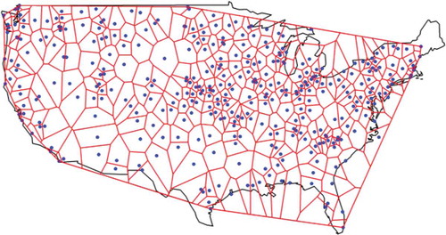
We use the Albers equal-area conic projection to map the data onto a flat plane and perform all subsequent calculations. However, all map visualizations in the figures of the manuscript are presented in an equi-rectangular map projection. After defining the convex hull of the 362 stations, we define all Thiessen polygons corresponding to each station. The Thiessen (also known as Voronoi or Dirichlet) tessellation is computed by functions in the spatstat and deldir R packages (Baddeley et al. 2015, Turner 2016, respectively) according to the second (iterative) algorithm of Lee and Schachter (1980). The mean annual temperature in the convex hull for the time period 1916–2015 is computed using the Thiessen polygon method.

3.2 Precipitation data

We use daily precipitation data from the Global Historical Climatology Network (GHCN, Menne et al. 2012a, 2012b). The initial dataset includes time series with missing or flagged (i.e. data of low quality for reasons explained in Menne et al. 2012a) values. We choose the stations with latitude in the interval [25°, 50°] and longitude in the interval [−125°, −65°] (USA region). We processed the dataset according to a sequence of actions briefly described in Appendix 4. The locations of the 319 stations that remain after the selection procedure are depicted in Figure 4.

Figure 4. Map of locations for the 319 stations with precipitation data (dots). Thiessen polygons for each station within the convex hull of the stations are also depicted.

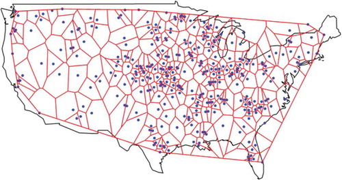
The definition of the convex hull of the stations and the methodology for the Thiessen polygons and the calculation of the spatial average precipitation over the convex hull are the same as those described in Section 3.1 for temperature.

3.3 GCM data

By GCM data we mean the GCM outputs for monthly temperature and precipitation from the CMIP5 experiment, which involves more than 50 GCMs modelled by 20 modelling groups (Taylor et al. 2012). Each model comes with its own spatial grid resolution. The models used in the present study and the variables of interest are presented in Table 1. Each GCM in Table 1 includes a simulation of the recent past (1850–2005) (historical run) and a future projection (2006–2100) forced by the representative concentration pathway 6.0 (RCP6). The RCP6 experiment represents a high concentration pathway in which stabilization of the radiative forcing at 6.0 W m⁻² occurs around 2100 and then forcing remains fixed (Masui et al. 2011, Meinshausen et al. 2011, Fig. 4). Most of the models have multiple ensemble members. Here we use the ensemble member r1i1p1 for each model.

Table 1. CMIP5 model acronyms, modelling groups and institutes, and variable of interest. The model outputs were downloaded from https://pcmdi.llnl.gov/search/cmip5/.

Model name	Temperature	Precipitation	Modelling centre (or group)	Institute ID
GISS-E2-H	✓	✓	NASA Goddard Institute for Space Studies	NASA GISS
GISS-E2-R	✓		NASA Goddard Institute for Space Studies	NASA GISS
HadGEM2-AO	✓	✓	National Institute of Meteorological Research/Korea Meteorological Administration	NIMR/KMA
IPSL-CM5A-LR	✓	✓	Institut Pierre-Simon Laplace	IPSL
IPSL-CM5A-MR	✓	✓	Institut Pierre-Simon Laplace	IPSL
MIROC5	✓	✓	Atmosphere and Ocean Research Institute (The University of Tokyo), National Institute for Environmental Studies, and Japan Agency for Marine-Earth Science and Technology	MIROC
MIROC-ESM	✓	✓	Japan Agency for Marine-Earth Science and Technology, Atmosphere and Ocean Research Institute (The University of Tokyo), and National Institute for Environmental Studies	MIROC
MIROC-ESM-CHEM	✓	✓	Japan Agency for Marine-Earth Science and Technology, Atmosphere and Ocean Research Institute (The University of Tokyo), and National Institute for Environmental Studies	MIROC
MRI-CGCM3	✓	✓	Meteorological Research Institute	MRI
NOAA GFDL GFDL-CM3	✓	✓	NOAA Geophysical Fluid Dynamics Laboratory	NOAA GFDL
NOAA GFDL GFDL-ESM2G	✓	✓	NOAA Geophysical Fluid Dynamics Laboratory	NOAA GFDL
NOAA GFDL GFDL-ESM2M	✓	✓	NOAA Geophysical Fluid Dynamics Laboratory	NOAA GFDL
NorESM1-M	✓	✓	Norwegian Climate Centre	NCC
NorESM1-ME	✓	✓	Norwegian Climate Centre	NCC

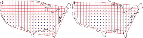
We extract GCM grid data corresponding to points within the respective convex hulls defined in Figures 3 and 4 and to the time period 1916–2100. Two examples of the Thiessen polygons formed from the GCM points within the convex hull, defined in Figure 3, are presented in Figure 5. The methodology for aggregating the temperature and precipitation over the convex hull is presented in Section 3.1.

Figure 5. Temperature (left) and precipitation (right) Thiessen polygons for each grid centre point (dot) for the GISS-E2-H model within the convex hull of the stations.

4 Application

In Section 4 we present the results of the model presented in Section 2.2 for controlled simulation data (for testing) and data of Section 3 (for prediction).

4.1 Framework testing using simulations

We test the performance of the BPF on simulated series with n₁ = 100 and n₂ = 50. The aim is to show the performance of the BPF even in extreme conditions. In Table 2 we present the types of simulated time series to which we applied the BPF. In Table 3 we present the estimated parameters of the BPF. Additionally, we present Pearson’s r of x_1(1:100) and x_2(1:100) and the respective values of the SC and the IS. In all examined cases we use the same simulated time series x_2(1:100), therefore the parameter σ has a common value. Thus, in all cases, the SC and IS provide the same amount of information.

Table 2. Simulated time series presented in the figures of Section 4.1.

Case	Figure	Variable	Simulation
1	Fig. 6 (top)	x1	HKp with μ = 0, σ = 0.40, H = 0.50 with added trend = 0.01
		x2	HKp with μ = 5, σ = 2, H = 0.70
2	Fig. 6 (bottom)	x1	Equal to x2 of case 1 in the period 1–100. Linear trend = 0.50 with starting point equal to (x2(100) of case 1 + 0.50) in the period 101–150
		x2	Equal to x2 of case 1
3	Fig. 7 (top)	x1	Equal to x2 of case 1 in the period 1–100. Linear trend = 0.10 with starting point equal to (x2(100) of case 1 + 0.10) in the period 101–150. In the resulting time series we add an HKp with μ = 0, σ = 1, H = 0.50
		x2	Equal to x2 of case 1
4	Fig. 7 (bottom)	x1	Equal to x2 of case 1 in the period 1–100. Linear trend = 0.10 with starting point equal to (x2(100) of case 1 + 0.10) in the period 101–150. In the resulting time series we add an HKp with μ = 0, σ = 1, H = 0.50 and we shift it up 5 units
		x2	Equal to x2 of case 1
5	Fig. 8 (top)	x1	HKp with μ = 5, σ = 2, H = 0.50 in the period 1–100. Linear trend = 0.10 with starting point equal to (x1(100) of the present case + 0.10) in the period 101–150
		x2	Equal to x2 of case 1
6	Fig. 8 (middle)	x1	Equal to x1 of case 6 in the period 1–100. Linear trend = 0.50 with starting point equal to (x1(100) of case 6 + 0.50) in the period 101–150
		x2	Equal to x2 of case 1
7	Fig. 8 (bottom)	x1	HKp with μ = 5, σ = 2, H = 0.50 in the period 1–100. Linear trend = 0.50 with starting point equal to (x1(100) of the present case + 0.50) in the period 101–150
		x2	Equal to x2 of case 1

Table 3. Estimates of the BPF parameters defined in Equations (14)–(16), (24), (25), (33) for the cases of Table 2. r is defined in Equation (37) and is estimated using sample Pearson’s r of x_1(1:100) and x_2(1:100). SC and IS are defined in Equations (34) and (35) and estimated by substituting σ, a, σ_e with their estimates. Cases with higher IS have a better ranking.

Case	Figure	μ	σ	H	a	b	σe	r	SC	IS	Ranking
1	Fig. 6 (top)	4.63	1.93	0.67	−0.05	0.81	0.54	−0.16	0.08	0.16	4
2	Fig. 6 (bottom)	4.63	1.93	0.67	1.00	0.00	0.00	1.00	∞	1.00	1
3	Fig. 7 (top)	4.63	1.93	0.67	0.99	0.03	1.11	0.86	0.89	0.86	3
4	Fig. 7 (bottom)	4.63	1.93	0.67	1.07	4.57	0.97	0.91	1.11	0.91	2
5	Fig. 8 (top)	4.63	1.93	0.67	−0.02	4.92	1.90	−0.02	0.01	0.02	6
6	Fig. 8 (middle)	4.63	1.93	0.67	−0.02	4.92	1.90	−0.02	0.01	0.02	7
7	Fig. 8 (bottom)	4.63	1.93	0.67	−0.06	6.41	1.95	−0.06	0.03	0.06	5

Figure 6 (top) shows the results of the application assuming: (a) x₂ follows a HKp, (b) a linear deterministic forecast model and (c) the deterministic forecast is of low quality (a is almost equal to 0 and IS is low). Pearson’s r is related to a and both are slightly negative. Therefore, the influence of the deterministic forecast on the probabilistic forecast is negligible.

Figure 6. The 95% prediction intervals produced by the BPF for the case of a time series (green) simulated from a HKp, when the deterministic model (blue) is of low quality (top) and perfect (bottom). The mean is equal to the estimated μ of the HKp model fitted to the observations of the period 1–100. The BPF is fitted on the period 1–100 and predicts for the period 101–150. The characteristics of the simulated time series are presented in Table 2, while the estimated parameters of the BPF are shown in Table 3.

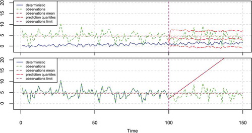
In the test application of Figure 6 (bottom), the assumptions are radically different. Here again x₂ follows a HKp, but the deterministic hindcast is assumed to be perfect (zero error and IS = 1). Furthermore, the deterministic forecast is assumed to be a huge linear trend. Because of the perfect performance of the deterministic model in the past, the BPF forecast fully complies with the deterministic model forecast (it is exactly equal and the 95% prediction interval has zero length in each time step). One could view this case as model testing in nonstationary conditions, because at time 100 the deterministic model fully changes its behaviour, yielding the huge linear trend, which did not appear before. Even though the BPF framework is founded on a fully stationary setting, it perfectly captures the assumed nonstationary behaviour. The reason is that the deterministic model is found to behave very well for the past; had it behaved badly, the probabilistic forecast (BPF) would disregard the linear trend and would be similar to that in Figure 6 (top).

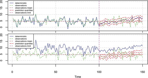
In the application depicted in Figure 7 (top), the deterministic hindcast is almost perfect (with a small, nonzero, error and a high IS). Here again (as in Fig. 6 (bottom)), the BPF forecast is strongly influenced by the deterministic forecast; however, now some prediction intervals of nonzero size appear. In the application depicted in Figure 7 (bottom), the deterministic hindcast and forecast of Figure 7 (top) have been shifted up. However, the BPF forecast has not changed. This shows that the BPF is invariant under the mean change, which is a desirable property. The meaning of this is that if the deterministic model has a systematic bias, however high, the BPF framework automatically removes it.

Figure 7. The 95% prediction intervals produced by the BPF for the case of a time series (green) simulated from a HKp with μ = 5, σ = 2 and H = 0.7, when the deterministic model (blue) is almost perfect and varies a bit around the observations (top), or is shifted up (bottom). The mean is equal to the estimated μ of the HKp model fitted to the observations of the period 1–100. The BPF is fitted in the period 1–100 and predicts for the period 101–150. The characteristics of the simulated time series are presented in Table 2, while the estimated parameters of the BPF are shown in Table 3.

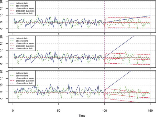
In the application depicted in Figure 8 (top), the deterministic hindcast is of low quality. Furthermore, a is slightly negative. In this case, the deterministic forecast is increasing while the BPF is slightly decreasing, which is reasonable because of the negative a. In Figure 8 (middle) the deterministic hindcast and observations are equal to those of Figure 8 (top). However, Figure 8 (middle) differs from Figure 8 (top) in that the deterministic forecast in the period {101, …, 150} increases faster, resulting in a faster decrease of the BPF forecast. In Figure 8 (bottom) a is even more negative, resulting in an even higher decrease of the BPF forecast. Finally, the IS provides a ranking of the models (cases) in terms of their informativeness (from the highest to the lowest), which in the examined cases is 2, 4, 3, 1, 7, 5 and 6.

Figure 8. The 95% prediction intervals produced by the BPF for the case of a time series (green) simulated from a HKp with μ = 5, σ = 2 and H = 0.7. The deterministic model (blue) is a simulated HKp with equal parameters, but of low quality in hindcast and a slight linear trend in forecast (top) or high trend (middle) and more negative correlation (bottom). The mean is equal to the estimated μ of the HKp model fitted to the observations of the period 1–100. The BPF is fitted in the period 1–100 and predicts for the period 101–150. The characteristics of the simulated time series are presented in Table 2, while the estimated parameters of the BPF are shown in Table 3.

Overall, all testing experiments indicate an ideal performance of the BPF framework in all cases, even the most extreme ones and those with huge nonstationary trends. The methodology presented complies with the simple truth of the scientific method that model predictions for the future are taken into account insofar as models comply with evidence from data of the past. Also, the methodology complies with the blueprint by Montanari and Koutsoyiannis (2012) insofar as it takes a deterministic model and incorporates it into a stochastic framework, thus converting the deterministic into stochastic predictions. If the deterministic model is good, the final stochastic prediction relies highly on it. If the model is bad, it is almost automatically discarded.

4.2 Case studies

In this section, we present the application of the BPF to the data of Section 3. We present two variants of the BPF, which are described in Sections 2.2 (Fig. 1) and 2.4 (Fig. 2) and the respective fitting and forecasting periods in Figure 9. In the case of Figure 9 (top), the GCM historical runs have already been adjusted using information from the observations, therefore using the time period 1916–2005 would use the same information twice. Instead, in the case of Figure 9 (bottom), the fitting of the BPF linear model in the time period 2006–2015 is based on a forecast with the assumptions of the RCP6 experiment regarding the emissions scenario, which have not been checked. In both cases, we use the HKp to model the observations.

Figure 9. BPF fitting and predicting time periods. The fitting period is defined as the period of the historical run (top) or the intersection of the historical observations and the RCP6 time periods (bottom). The prediction period succeeds the fitting period and extends to the year 2100.

We present the results in Figures 10–15. In all figures the mean of the observations is equal to the maximum likelihood estimate of μ, as given in Section 2.5 for the fitting time period. While we examined all GCMs of Table 1, we present here in detail two of them, i.e. the GISS-E2-H and the MRI-CGCM3, along with summary information for all results. Figure 10 shows the prediction of the mean annual temperature in the USA for the two GCMs when the fitting time period is 1916–2005. In the case of the GISS-E2-H model the forecasted increase is equal to 0.8°C while the 95% prediction interval is 1.8°C wide. In the case of the MRI-CGCM3 model, the forecasted increase is negligible while the 95% prediction interval is again 1.8°C wide. In Figure 11, the prediction intervals for the fitting time period 2006–2015 indicate a mean increase in the annual temperature equal to 1.4°C and 0.9°C for the two models, respectively, while the respective prediction intervals are 2.0°C wide.

Figure 10. The 95% prediction intervals of the mean annual temperature in the USA produced by the BPF for the case of Figure 9 (top). The fitting time period is 1916–2005, while the deterministic models are ensembles from the GISS-E2-H (top) and MRI-CGCM3 (bottom) models. The mean of the observations is equal to the maximum likelihood estimate of μ in Section 2.5 for the fitting time period.

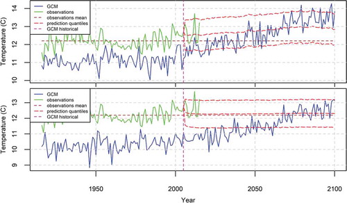
Figure 11. The 95% prediction intervals of the mean annual temperature in the USA produced by the BPF for the case of Figure 9 (bottom). The fitting time period is 2006–2015, while the deterministic models are ensembles from the GISS-E2-H (top) and MRI-CGCM3 (bottom) models.

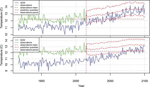
Figure 12. The 95% prediction intervals of the annual precipitation in the USA produced by the BPF for the case of Figure 9 (top). The fitting time period is 1916–2005, while the deterministic models are ensembles from the GISS-E2-H (top) and MRI-CGCM3 (bottom) models.

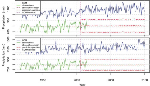
Figure 13. The 95% prediction intervals of the annual precipitation in the USA produced by the BPF for the case of Figure 9 (bottom). The fitting time period is 2006–2015, while the deterministic models are ensembles from the GISS-E2-H (top) and MRI-CGCM3 (bottom) models.

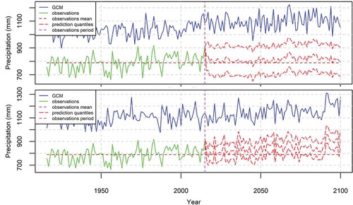
Figure 14. Prediction intervals of the mean annual temperature in the USA produced by the BPF. The GCM medians correspond to all GCMs of Table 1. The prediction quantiles are the envelopes of all the 95% prediction intervals of the GCMs of Table 1 produced by the BPF. The fitting time period is 1916–2005 (top, corresponds to Fig. 9 (top)) and 2006–2015 (bottom, corresponds to Fig. 9 (bottom)).

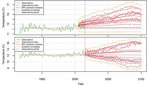
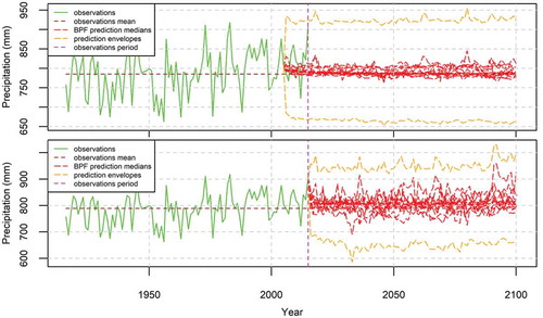
Figure 15. Prediction intervals of the annual precipitation in the USA produced by the BPF. The GCM medians correspond to all GCMs of Table 1. The prediction quantiles are the envelopes of all the 95% prediction intervals of the GCMs of Table 1 produced by the BPF. The fitting time period is 1916–2005 (top, corresponds to Fig. 9 (top)) and 2006–2015 (bottom, corresponds to Fig. 9 (bottom)).

Figures 12 and 13 depict similar results for the annual precipitation in the USA. In particular, in Figure 12, which shows the results for the fitting time period 1916–2005, we observe a negligible increase of the annual precipitation, while the 95% prediction intervals are 200 mm wide. In Figure 13, where the fitting time period is 2006–2015, we observe an insignificant increase and a mean annual increase of 120 mm, respectively, while the respective 95% prediction intervals are 220 and 140 mm wide.

Figures 14 and 15 display the results for all models of Table 1. In particular, they show the forecasted mean annual temperatures and annual precipitations for both method variants defined in Figure 9. Furthermore, the graphs include the envelopes of all 95% prediction intervals. In Figure 14, we observe an envelope of the mean annual temperature 5.8°C wide when the fitting time period is 1916–2005, and an envelope 8.8°C wide when the fitting time period is 2006–2015. In the former case, the temperature increase is centred around 2.5°C for the year 2100, while in the latter case the mean annual change seems to be negligible, while the overall shape of the graph could be called a “Bayesian thistle”. Regarding the precipitation, we observe in Figure 15 envelopes 270 and 330 mm wide for the fitting time periods 1916–2005 and 2006–2015, respectively. The forecasted increase in precipitation is negligible in the former case, while it is approximately equal to 50 mm for the year 2100 in the latter case.

5 Conclusions

The aim of this paper is to probabilistically predict the future evolution of a normal stationary stochastic process used to model a geophysical variable conditional on historical observations of the variable and hindcasts and forecasts of the variable produced by a deterministic model. To this end, we apply the Bayesian processor of forecasts (BPF) to the data of interest. The BPF has previously been applied to independent variables or Markovian processes. Here, we extend its use to include any normal stationary stochastic processes and we present an application to the special case of the Hurst-Kolmogorov process.

We investigate the properties of the BPF and test its performance using simulated time series. We show that the influence of the deterministic forecast increases when there is a good fitting of the deterministic model to the historical observations. Indeed, when this fitting is perfect, the BPF forecast is equal to the deterministic forecast. In contrast, when this fitting is insufficient, the forecast depends on the observations and the stochastic model and not on the deterministic model. Furthermore, even if the stochastic model is stationary, the BPF can incorporate changes, which can be attributed to nonstationarity.

The BPF is applied to the mean annual temperature and annual precipitation in the time period 1916–2005 in the USA. The GCMs (the historical and the RCP6 scenarios) are used as deterministic models. Using the estimated BPF parameters, we probabilistically forecast the mean annual temperature and annual precipitation until the year 2100. The results are sensitive to the choice of the fitting period between the observations and the deterministic forecast and the choice of the GCM model. Regarding the temperature, the overall results show increasing temperature when the fitting period is the intersection of the data time period and the historical scenario, while the temperature remains unchanged when the fitting period is the intersection of the data time period and the RCP6 scenario. In both cases, the envelopes of the 95% prediction intervals for each GCM model are significantly wide (5.8°C and 8.8°C, respectively). Regarding the precipitation, the deterministic models had a negligible effect on improving the forecast of the stochastic model, regardless of the fitting period.

We emphasize that the estimation of the stochastic model parameters would be better performed using only data that were not used in the GCM fitting/tuning, i.e. for the period after 2006. This would correspond to the so-called split-sample technique (Klemeš 1986), which avoids possible model overfitting on the available data and thus artificially good performance. This corresponds to the model fitting period after 2006. The applications with this variant of the methodology show that the uncertainty of the forecasts increases considerably and practically result in total neglect of the GCM predictions regarding both temperature and precipitation. Finally, the inclusion of the uncertainty in a fully Bayesian setting, also considering the uncertainty of parameters, would result in even higher uncertainties of the forecasted variables.

Acknowledgment

We acknowledge two anonymous reviewers whose suggestions as well as comments, both positive and negative, helped to improve the manuscript. We acknowledge the World Climate Research Programme’s Working Group on Coupled Modelling, which is responsible for CMIP, and we thank the climate modelling groups (listed in Table 1 of this paper) for producing and making available their model outputs. For CMIP the US Department of Energy’s Program for Climate Model Diagnosis and Intercomparison provides coordinating support and led development of software infrastructure in partnership with the Global Organization for Earth System Science Portals.

Disclosure statement

No potential conflict of interest was reported by the authors.

Additional information

Funding

The authors received no funding for this research, which was performed for scientific curiosity.

Appendices

Appendix 1. The Bayesian processor of forecasts applied to normal stationary stochastic processes

Here we prove the results presented in Section 2.2. Overall, we prefer to use techniques typically met in the Bayesian statistics literature, such as proportionality of the distributions, and avoid calculating integrals. For example, Marty et al. (2015) used these techniques when they examined the Bayesian processor of output, while Krzysztofowicz (1985) preferred the other way when he examined the BPF.

Let x₁ and x₂ and their subsets y₁, y₂, y₃, y₄ be defined as follows:

(A.1)

(A.2)

(A.3)

(A.4)

(A.5)

(A.6)

(A.7)

(A.8)

Then the conditional independence mentioned in Section 2.1 is defined by:

(A.9)

(A.10)

which results in:

(A.11)

Hence:

(A.12)

(A.13)

(A.14)

(A.15)

(A.16)

(A.17)

Equation (A.17) proves Equation (13).

We define the parameters of the normal stationary stochastic process used to model the observations with Equations (A.18)–(A.28). Matrices Σ and R and their submatrices are symmetric Toeplitz positive definite matrices (Golub and Van Loan 1996, p. 193). This facilitates their handling using the Levinson or related algorithms (e.g. Tyralis and Koutsoyiannis 2011). Consequently:

(A.18)

(A.19)

(A.20)

(A.21)

(A.22)

(A.23)

(A.24)

(A.25)

(A.26)

(A.27)

(A.28)

Since we model x₂ with a multivariate normal distribution, the distribution of y₄ conditional on y₃ is given by (Eaton 2007, p. 116):

(A.29)

which can be written as

(A.30)

where

(A.31)

(A.32)

whereas Equation (A.32) denotes the Schur complement (Horn and Zhang 2005).

If the distribution of x_1n conditional on x_2n is given by:

(A.33)

then, using Equation (A.11) and the properties of the product of normal distributions (Bromiley 2014), we find:

(A.34)

(A.35)

(A.36)

where

(A.37)

(A.38)

However, in the Bayesian setting, y₂ is known while the distribution of interest is that of y₄|y₂. Therefore, Equation (A.36) is transformed to Equation (A.45) in which y₄ is the random variable and y₂ is a value, after some algebraic manipulations:

(A.39)

(A.40)

(A.41)

(A.42)

(A.43)

(A.44)

(A.45)

where

(A.46)

(A.47)

The distribution of y₄|y₃, x₁ in Equation (A.17) is normal:

(A.48)

because it is proportional to the product of the two normal distributions (A.30) and (A.45) (Bromiley 2014). Its parameters are given by Equations (A.50) and (A.54) after the following manipulations:

(A.49)

(A.50)

(A.51)

(A.52)

(A.53)

(A.54)

Appendix 2. The Bayesian processor of forecasts applied to distinct fitting periods

Here we repeat the procedure of Appendix 1 but for distinct fitting periods. The time period {1,…, n₁ + n₂ + n₃} is divided into three subperiods . The processes of interest are x₁ and x₂ and their subsets y₁, y₂, y₃, y₄, y₅, y₆ defined as:

(B.1)

(B.2)

(B.3)

(B.4)

(B.5)

(B.6)

(B.7)

(B.8)

(B.9)

(B.10)

Then the conditional independence mentioned in Section 2.1 is defined by:

(B.11)

(B.12)

which result in:

(B.13)

Hence:

(B.14)

(B.15)

(B.16)

(B.17)

(B.18)

(B.19)

We define the parameters of the normal stationary stochastic process used to model the observations through the following equations:

(B.20)

(B.21)

(B.22)

(B.23)

(B.24)

(B.25)

(B.26)

(B.27)

(B.28)

(B.29)

(B.30)

Since we model x₂ with a multivariate normal distribution, the distribution of y₅ conditional on y₃ and y₄ is given by (Eaton 2007, p. 116):

(B.31)

which can be written as

(B.32)

where

(B.33)

(B.34)

If the distribution of x_1n conditional on x_2n is given by

(B.35)

then, using Equation (B.13) and the properties of the product of normal distributions (Bromiley 2014), we find:

(B.36)

(B.37)

(B.38)

where

(B.39)

(B.40)

However, in the Bayesian setting y₂ is given while the distribution of interest is that of y₅|y₂. Therefore, Equation (B.38) is transformed to Equation (B.47) in which y₅ is the random variable and y₂ is a value, after some algebraic manipulations:

(B.41)

(B.42)

(B.43)

(B.44)

(B.45)

(B.46)

(B.47)

(B.48)

(B.49)

The distribution of in Equation (B.19) is normal:

(B.50)

because it is proportional to the product of the two normal distributions (B.32) and (B.47) (Bromiley 2014). Its parameters are given by Equations (B.52) and (B.56) according to the following manipulations:

(B.51)

(B.52)

(B.53)

(B.54)

(B.55)

(B.56)

Appendix 3. Investigation of the BPF for various values of its parameters

From Equation (A.49) we obtain:

(C.1)

while from Equations (A.52) and (C.1) we obtain:

(C.2)

In the case where

(C.3)

using Equations (C.1) and (C.2), we obtain:

(C.4)

(C.5)

In the case where

(C.6)

we find that

(C.7)

Hence, from Equations (A.17) and (A.30) we obtain:

(C.8)

Appendix 4. Precipitation data

Here we present the sequence of steps to aggregate the precipitation from the daily to the annual scale. This sequence is reproduced from Tyralis et al. (2017), who use the same dataset and procedures.

A. Flagged values were considered as missing values.

B. Months with a percentage of recorded values higher than 0.83 (i.e. with more than 25/30 or 26/31 daily observations) are considered good, while months with a percentage of recorded values less than 0.34 (i.e. equal to or less than 10/30 and 10/31 daily observations) are considered of poor quality. The reason for the differentiation is that we first aggregate to the monthly time scale and then to the annual time scale. Thus, even if all values in a month are missing we can fill the monthly value after the first aggregation, as described in step C.

B1. Missing values within months with observed values more than 83% were filled using linear interpolation.

B2. All values within months with observed values less than 34% were considered as missing.

B3. For the rest of the months the missing values were filled in using linear interpolation and then these months were considered as missing. The reason is explained in step D.

C. Missing months corresponding to steps B2 and B3 (the latter after the substitution with missing values) were filled in using a seasonal Kalman filter, implemented in the R package zoo (Zeileis and Grothendieck 2005).

D. Mean monthly values for months in which both steps B3 and C (i.e. months with missing values more than 34% and less than 83%) were applied were calculated with the mean of monthly values of steps B3 and C.

E. From the mean monthly values we obtained the mean annual values.

F. Finally we discarded annual time series if one of the following constraints was satisfied:

F1. Two or more missing years.

F2. Hurst parameter estimate H ≥ 0.95, mean annual rainfall μ ≥ 3000 mm, standard deviation of annual rainfall σ ≥ 750 mm, coefficient of variation of annual rainfall c_v ≥ 0.8. These constraints on the estimated parameters were justified from a preliminary analysis, which showed that higher values were outliers.

F3. Four or more years with less than 60% of observed daily values.

References

- Aloysius, N.R., et al., 2016. Evaluation of historical and future simulations of precipitation and temperature in central Africa from CMIP5 climate models. Journal of Geophysical Research, 121 (1), 130–152. doi:10.1002/2015JD023656
- Anagnostopoulos, G.G., et al., 2010. A comparison of local and aggregated climate model outputs with observed data. Hydrological Sciences Journal, 55 (7), 1094–1110. doi:10.1080/02626667.2010.513518
- Baddeley, A., Rubak, E., and Turner, R., 2015. Spatial point patterns: methodology and applications with R. London: Chapman and Hall/CRC Press.
- Bromiley, P., 2014. Products and convolutions of Gaussian probability density functions. University of Manchester, Tina Memo No. 2003-003 [online]. Available from: http://tina.wiau.man.ac.uk/docs/memos/2003-003.pdf
- Chen, F., Jiao, M., and Chen, J., 2013. The meta-Gaussian Bayesian Processor of forecasts and associated preliminary experiments. Acta Meteorologica Sinica, 27 (2), 199–210. doi:10.1007/s13351-013-0205-9
- Chowdhury, S. and Sharma, A., 2011. Global sea surface temperature forecasts using a pairwise dynamic combination approach. Journal of Climate, 24, 1869–1877. doi:10.1175/2010JCLI3632.1
- de Finetti, B., 1974. Theory of probability. New York: Wiley.
- Dessai, S. and Hulme, M., 2004. Does climate adaptation policy need probabilities? Climate Policy, 4 (2), 107–128. doi:10.1080/14693062.2004.9685515
- Eaton, M.L., 2007. Multivariate statistics: a vector space approach. Lecture Notes-Monograph Series. Volume. 53. Beachwood, OH: Institute of Mathematical Statistics.
- Ehret, U., et al., 2012. HESS opinions “Should we apply bias correction to global and regional climate model data?”. Hydrology and Earth System Sciences, 16, 3391–3404. doi:10.5194/hess-16-3391-2012
- Fatichi, S., Ivanov, V.Y., and Caporali, E., 2012. Investigating interannual variability of precipitation at the global scale: is there a connection with seasonality? Journal of Climate, 25, 5512–5523. doi:10.1175/JCLI-D-11-00356.1
- Golub, G.H. and Van Loan, C.F., 1996. Matrix computations. 3rd ed. Baltimore: John Hopkins University Press.
- Groves, D.G., Yates, D., and Tebaldi, C., 2008. Developing and applying uncertain global climate change projections for regional water management planning. Water Resources Research, 44, 12. doi:10.1029/2008WR006964
- Hawkins, E., et al., 2014. Uncertainties in the timing of unprecedented climates. Nature, 511, E3–E5. doi:10.1038/nature13523
- Hawkins, E. and Sutton, R., 2009. The potential to narrow uncertainty in regional climate predictions. Bulletin of the American Meteorological Society, 90, 1095–1107. doi:10.1175/2009BAMS2607.1
- Hawkins, E. and Sutton, R., 2011. The potential to narrow uncertainty in projections of regional precipitation change. Climate Dynamics, 37 (1), 407–418. doi:10.1007/s00382-010-0810-6
- Hemelrijk, J., 1966. Underlining random variables. Statistica Neerlandica, 20 (1), 1–7. doi:10.1111/j.1467-9574.1966.tb00488.x
- Hewitt, A.J., et al., 2016. Sources of uncertainty in future projections of the carbon cycle. Journal of Climate, 29, 7203–7213. doi:10.1175/JCLI-D-16-0161.1
- Hibbard, K.A., et al., 2007. A strategy for climate change stabilization experiments. Eos, Transactions American Geophysical Union, 88 (20), 217–221. doi:10.1029/2007EO200002
- Horn, R.A. and Zhang, F., 2005. Basic properties of the Schur complement. In: F. Zhang, ed. The Schur complement and its applications. New York: Springer US. doi:10.1007/b105056
- Horrace, W.C., 2005. Some results on the multivariate truncated normal distribution. Journal of Multivariate Analysis, 94 (1), 209–221. doi:10.1016/j.jmva.2004.10.007
- Iliopoulou, T., et al., 2016. Revisiting long-range dependence in annual precipitation. Journal of Hydrology. doi:10.1016/j.jhydrol.2016.04.015
- Johnson, F. and Sharma, A., 2009. Measurement of GCM skill in predicting variables relevant for hydroclimatological assessments. Journal of Climate, 22, 4373–4382. doi:10.1175/2009JCLI2681.1
- Katz, R.W., 2002. Techniques for estimating uncertainty in climate change scenarios and impact studies. Climate Research, 20, 167–185. doi:10.3354/cr020167
- Klemeš, V., 1986. Operational testing of hydrological simulation models. Hydrological Sciences Journal, 1, 13–24. doi:10.1080/02626668609491024
- Knutti, R. and Sedláček, J., 2013. Robustness and uncertainties in the new CMIP5 climate model projections. Nature Climate Change, 3, 369–373. doi:10.1038/nclimate1716
- Koutroulis, A.G., et al., 2015. Evaluation of precipitation and temperature simulation performance of the CMIP3 and CMIP5 historical experiments. Climate Dynamics, 47 (5), 1881–1898. doi:10.1007/s00382-015-2938-x
- Koutsoyiannis, D., 2002. The Hurst phenomenon and fractional Gaussian noise made easy. Hydrological Sciences Journal, 47 (4), 573–595. doi:10.1080/02626660209492961
- Koutsoyiannis, D., 2003. Climate change, the Hurst phenomenon, and hydrological statistics. Hydrological Sciences Journal, 48 (1), 3–24. doi:10.1623/hysj.48.1.3.43481
- Koutsoyiannis, D., 2006a. A toy model of climatic variability with scaling behaviour. Journal of Hydrology, 322 (1–4), 25–48. doi:10.1016/j.jhydrol.2005.02.030
- Koutsoyiannis, D., 2006b. Nonstationarity versus scaling in hydrology. Journal of Hydrology, 324 (1–4), 239–254. doi:10.1016/j.jhydrol.2005.09.022
- Koutsoyiannis, D., et al., 2008a. On the credibility of climate predictions. Hydrological Sciences Journal, 53 (4), 671–684. doi:10.1623/hysj.53.4.671
- Koutsoyiannis, D., Efstratiadis, A., and Georgakakos, K.P., 2007. Uncertainty assessment of future hydroclimatic predictions: a comparison of probabilistic and scenario-based approaches. Journal of Hydrometeorology, 8 (3), 261–281. doi:10.1175/JHM576.1
- Koutsoyiannis, D. and Montanari, A., 2007. Statistical analysis of hydroclimatic time series: uncertainty and insights. Water Resources Research, 43 (5), W05429. doi:10.1029/2006WR005592
- Koutsoyiannis, D. and Montanari, A., 2014. Negligent killing of scientific concepts: the stationarity case. Hydrological Sciences Journal, 60 (7–8), 1174–1183. doi:10.1080/02626667.2014.959959
- Koutsoyiannis, D., Yao, H., and Georgakakos, A., 2008b. Medium-range flow prediction for the Nile: a comparison of stochastic and deterministic methods. Hydrological Sciences Journal, 53 (1), 142–164. doi:10.1623/hysj.53.1.142
- Krzysztofowicz, R., 1985. Bayesian models of forecasted time series. Journal of the American Water Resources Association, 21 (5), 805–814. doi:10.1111/j.1752-1688.1985.tb00174.x
- Krzysztofowicz, R., 1987. Markovian forecast processes. Journal of the American Statistical Association, 82 (397), 31–37. doi:10.2307/2289121
- Krzysztofowicz, R., 1992. Bayesian correlation score: a utilitarian measure of forecast skill. Monthly Weather Review, 120, 208–220. doi:10.1175/1520-0493(1992)120<0208:BCSAUM>2.0.CO;2
- Krzysztofowicz, R., 1999a. Bayesian forecasting via deterministic model. Risk Analysis, 19 (4), 739–749. doi:10.1111/j.1539-6924.1999.tb00443.x
- Krzysztofowicz, R., 1999b. Bayesian theory of probabilistic forecasting via deterministic hydrologic model. Water Resources Research, 35 (9), 2739–2750. doi:10.1029/1999WR900099
- Krzysztofowicz, R., 2001. Integrator of uncertainties for probabilistic river stage forecasting: precipitation-dependent model. Journal of Hydrology, 249 (1–4), 69–85. doi:10.1016/S0022-1694(01)00413-9
- Krzysztofowicz, R., 2002. Bayesian system for probabilistic river stage forecasting. Journal of Hydrology, 268 (1–4), 16–40. doi:10.1016/S0022-1694(02)00106-3
- Krzysztofowicz, R., 2010. Decision criteria, data fusion and prediction calibration: a Bayesian approach. Hydrological Sciences Journal, 55 (6), 1033–1050. doi:10.1080/02626667.2010.505894
- Krzysztofowicz, R. and Evans, W.B., 2008. The role of climatic autocorrelation in probabilistic forecasting. Monthly Weather Review, 136 (12), 4572–4592. doi:10.1175/2008MWR2375.1
- Krzysztofowicz, R. and Maranzano, C.J., 2004. Bayesian system for probabilistic stage transition forecasting. Journal of Hydrology, 299 (1–2), 15–44. doi:10.1016/j.jhydrol.2004.02.013
- Kundzewicz, Z.W. and Stakhiv, E.Z., 2010. Are climate models “ready for prime time” in water resources management applications, or is more research needed? Hydrological Sciences Journal, 55 (7), 1085–1089. doi:10.1080/02626667.2010.513211
- Lawrimore, J.H., et al., 2011. An overview of the global historical climatology network monthly mean temperature data set, version 3. Journal of Geophysical Research, 116, D19121. doi:10.1029/2011JD016187
- Lee, D.T. and Schachter, B.J., 1980. Two algorithms for constructing a Delaunay triangulation. International Journal of Computer & Information Sciences, 9 (3), 219–242. doi:10.1007/BF00977785
- Macilwain, C., 2014. A touch of the random. Science, 344 (6189), 1221–1223. doi:10.1126/science.344.6189.1221
- Maloney, E.D., et al., 2014. North American climate in CMIP5 experiments: part III: assessment of twenty-first-century projections. Journal of Climate, 27, 2230–2270. doi:10.1175/JCLI-D-13-00273.1
- Markonis, Y. and Koutsoyiannis, D., 2016. Scale-dependence of persistence in precipitation records. Nature Climate Change, 6, 399–401. doi:10.1038/nclimate2894
- Marty, R., et al., 2015. Combining the Bayesian processor of output with Bayesian model averaging for reliable ensemble forecasting. Journal of the Royal Statistical Society C, 64 (1), 75–92. doi:10.1111/rssc.12062
- Masui, T., et al., 2011. An emission pathway for stabilization at 6 Wm−2 radiative forcing. Climatic Change, 109, 59–76. doi:10.1007/s10584-011-0150-5
- Matthes, J.H., et al., 2016. Benchmarking historical CMIP5 plant functional types across the Upper Midwest and Northeastern United States. Journal of Geophysical Research, 121 (2), 523–535. doi:10.1002/2015JG003175
- Meinshausen, M., et al., 2011. The RCP greenhouse gas concentrations and their extensions from 1765 to 2300. Climatic Change, 109, 213–241. doi:10.1007/s10584-011-0156-z
- Menne, M.J., et al., 2012a. Global historical climatology network - daily (GHCN-Daily), version 3.22. NOAA National Climatic Data Center. doi:10.7289/V5D21VHZ
- Menne, M.J., et al., 2012b. An overview of the global historical climatology network-daily database. Journal of Atmospheric and Oceanic Technology, 29, 897–910. doi:10.1175/JTECH-D-11-00103.1
- Montanari, A. and Grossi, G., 2008. Estimating the uncertainty of hydrological forecasts: a statistical approach. Water Resources Research, 44 (12), W00B08. doi:10.1029/2008WR006897
- Montanari, A. and Koutsoyiannis, D., 2012. A blueprint for process-based modelling of uncertain hydrological systems. Water Resources Research, 48, 9. doi:10.1029/2011WR011412
- Montanari, A. and Koutsoyiannis, D., 2014. Modeling and mitigating natural hazards: stationarity is immortal!. Water Resources Research, 50, 9748–9756. doi:10.1002/2014WR016092
- Moss, R.H., et al., 2010. The next generation of scenarios for climate change research and assessment. Nature, 463, 747–756. doi:10.1038/nature08823
- Nasrollahi, N., et al., 2015. How well do CMIP5 climate simulations replicate historical trends and patterns of meteorological droughts? Water Resources Research, 51 (4), 2847–2864. doi:10.1002/2014WR016318
- Notz, D., 2015. How well must climate models agree with observations?. Philosophical Transactions of the Royal Society A, 373, 2052. doi:10.1098/rsta.2014.0164
- Pirtle, Z., Meyer, R., and Hamilton, A., 2010. What does it mean when climate models agree? A case for assessing independence among general circulation models. Environmental Science & Policy, 13 (5), 351–361. doi:10.1016/j.envsci.2010.04.004
- Pokhrel, P., Robertson, D.E., and Wang, Q.J., 2013. A Bayesian joint probability post-processor for reducing errors and quantifying uncertainty in monthly streamflow predictions. Hydrology and Earth Systems Sciences, 17, 795–804. doi:10.5194/hess-17-795-2013
- Potter, K., et al., 2009. Visualization of uncertainty and ensemble data: exploration of climate modeling and weather forecast data with integrated ViSUS-CDAT systems. Journal of Physics: Conference Series, 180 (012089). doi:10.1088/1742-6596/180/1/012089
- Santer, B.D., et al., 2013. Identifying human influences on atmospheric temperature. Proceedings of the National Academy of Sciences of the United States of America, 110 (1), 26–33. doi:10.1073/pnas.1210514109
- Schneider, S.H., 2002. Can we estimate the likelihood of climatic changes at 2100? Climatic Change, 52 (4), 441–451. doi:10.1023/A:1014276210717
- Sheffield, J., et al., 2013a. North American climate in CMIP5 experiments. Part I: evaluation of historical simulations of continental and regional climatology. Journal of Climate, 26, 9209–9245. doi:10.1175/JCLI-D-12-00592.1
- Sheffield, J., et al., 2013b. North American climate in CMIP5 experiments. Part II: evaluation of historical simulations of intraseasonal to decadal variability. Journal of Climate, 26, 9247–9290. doi:10.1175/JCLI-D-12-00593.1
- Smith, P.J., et al., 2012. Adaptive correction of deterministic models to produce probabilistic forecasts. Hydrology and Earth Systems Sciences, 16, 2783–2799. doi:10.5194/hess-16-2783-2012
- Smith, R.L., et al., 2009. Bayesian modeling of uncertainty in ensembles of climate models. Journal of the American Statistical Association, 104 (485), 97–116. doi:10.1198/jasa.2009.0007
- Strobach, E. and Bel, G., 2015. Improvement of climate predictions and reduction of their uncertainties using learning algorithms. Atmospheric Chemistry and Physics, 15, 8631–8641. doi:10.5194/acp-15-8631-2015
- Taylor, K.E., Stouffer, R.J., and Meehl, G.A., 2012. An overview of CMIP5 and the experiment design. Bulletin of the American Meteorological Society, 93, 485–498. doi:10.1175/BAMS-D-11-00094.1
- Tian, D., Guo, Y., and Dong, W., 2015. Future changes and uncertainties in temperature and precipitation over China based on CMIP5 models. Advances in Atmospheric Sciences, 32 (4), 487–496. doi:10.1007/s00376-014-4102-7
- Turner, R., 2016. deldir: delaunay triangulation and Dirichlet (Voronoi) tessellation. R package version 0.1-12 [online]. Available from: https://CRAN.R-project.org/package=deldir
- Tyralis, H., 2016. HKprocess: Hurst-Kolmogorov process. R package version 0.0-2 [online]. Available from: https://CRAN.R-project.org/package=HKprocess
- Tyralis, H., et al., 2017. On the long-range dependence properties of annual precipitation using a global network of instrumental measurements. In review.
- Tyralis, H. and Koutsoyiannis, D., 2011. Simultaneous estimation of the parameters of the Hurst-Kolmogorov stochastic process. Stochastic Environmental Research & Risk Assessment, 25 (1), 21–33. doi:10.1007/s00477-010-0408-x
- Tyralis, H. and Koutsoyiannis, D., 2014. A Bayesian statistical model for deriving the predictive distribution of hydroclimatic variables. Climate Dynamics, 42 (11–12), 2867–2883. doi:10.1007/s00382-013-1804-y
- Uusitalo, L., et al., 2015. An overview of methods to evaluate uncertainty of deterministic models in decision support. Environmental Modelling & Software, 63, 24–31. doi:10.1016/j.envsoft.2014.09.017
- Wang, Q.J., Robertson, D.E., and Chiew, F.H.S., 2009. A Bayesian joint probability modeling approach for seasonal forecasting of streamflows at multiple sites. Water Resources Research, 45 (5), W05407. doi:10.1029/2008WR007355
- Wei, W.W.S., 2006. Time series analysis, univariate and multivariate methods. 2nd ed. Boston, MA: Pearson Addison Wesley.
- Woldemeskel, F.M., et al., 2014. A framework to quantify GCM uncertainties for use in impact assessment studies. Journal of Hydrology, 519 (Part B), 1453–1465. doi:10.1016/j.jhydrol.2014.09.025
- Xu, J., Powell Jr, A.M., and Zhao, L., 2013. Intercomparison of temperature trends in IPCC CMIP5 simulations with observations, reanalyses and CMIP3 models. Geoscientific Model Development, 6, 1705–1714. doi:10.5194/gmd-6-1705-2013
- Yip, S., et al., 2011. A simple, coherent framework for partitioning uncertainty in climate predictions. Journal of Climate, 24, 4634–4643. doi:10.1175/2011JCLI4085.1
- Ylhäisi, J.S., et al., 2015. Quantifying sources of climate uncertainty to inform risk analysis for climate change decision-making. Local Environment, 20 (7), 811–835. doi:10.1080/13549839.2013.874987
- Zeileis, A. and Grothendieck, G., 2005. zoo: S3 infrastructure for regular and irregular time series. Journal of Statistical Software, 14 (6), 1–27. doi:10.18637/jss.v014.i06
- Zhao, L., et al., 2011. A hydrologic post-processor for ensemble streamflow predictions. Advances in Geosciences, 29, 51–59. doi:10.5194/adgeo-29-51-2011
- Zhao, L., et al., 2015b. Uncertainties of the global-to-regional temperature and precipitation simulations in CMIP5 models for past and future 100 years. Theoretical and Applied Climatology, 122 (1), 259–270. doi:10.1007/s00704-014-1293-x
- Zhao, T., et al., 2015a. Quantifying predictive uncertainty of streamflow forecasts based on a Bayesian joint probability model. Journal of Hydrology, 528, 329–340. doi:10.1016/j.jhydrol.2015.06.043