Methodology to set trigger levels in an urban drainage flood warning system – an application to Jhonghe, Taiwan

ABSTRACT

A wireless water-level monitoring system for an urban drainage flood warning is developed, and stations equipped with pressure sensors are installed to monitor water levels. The water levels for flood warning are investigated. Two stages of warning water level for “larger” conduits are set based on the rate of rising water levels. In a similar way, only one stage of the warning water level is set for “smaller” conduits. The average rates of rising water levels for different scenarios are estimated using the US EPA Storm Water Management Model (SWMM). When evaluating the impact of flooding, the outflows from manholes simulated by the SWMM are used as sources for a two-dimensional overland flow simulation. The integrated system is successfully executed in Jhonghe, New Taipei City, Taiwan, which has experienced urban drainage floods. Therefore, this system can provide urban drainage flood warnings to the authorities to take disaster reduction measures.

KEYWORDS:

• trigger
• urban
• drainage
• flood
• warning
• wireless

Editor M.C. Acreman Associate editor E. Volpi

1 Introduction

In recent years, intensive rainfall has induced urban flooding in many metropolises, such as torrential rain-induced floods in Hong Kong, China (October 2016), and in Beijing, China (July 2016). Heavy rainfall and typhoons are characteristics of the climate in the circum-Pacific area. For example, the average annual rainfall in Taiwan is about 2500 mm, and more than 78% of the precipitation is concentrated in the monsoon and typhoon season from May to October (WRA 2008). The non-uniformity of rainfall is rather significant due to the topographic effect in Taiwan. Urban areas, which lack detention basins, usually experience a great deal of damage when the intense rainfall-induced discharge exceeds the design capacity of the urban drainage system. In 2001, Typhoon Nari brought heavy rainfall of 95–120 mm/h, which exceeded the ability of the system designed to handle only 45 mm/h of urban drainage in the Tamshui River basin. This event created a flood area of 6317 ha with a depth of 0.3–8.5 m (WRA 2001). Although flood warning systems for rivers are widely established throughout the world, urban drainage flood warning systems are few due to the nature of quick occurrence. This paper is aimed at creating an urban drainage flood warning system using wireless water-level monitoring.

The Tamshui River basin is located in northern Taiwan and is the most populated area in Taiwan (Fig. 1). One of the main reasons for flooding in this urban area is the amount of rainfall exceeding the drainage capacity. In the past, torrential rains induced by typhoons have usually caused a lot of damage due to insufficient response times to the overflow of manholes in the urban area of the Tamshui River basin (Cheng et al. 2007). Consequently, flood warnings may save lives, livestock and properties and are one of the crucial measures needed for flood mitigation to reduce damage in inundation-prone areas (NOAA 1997).

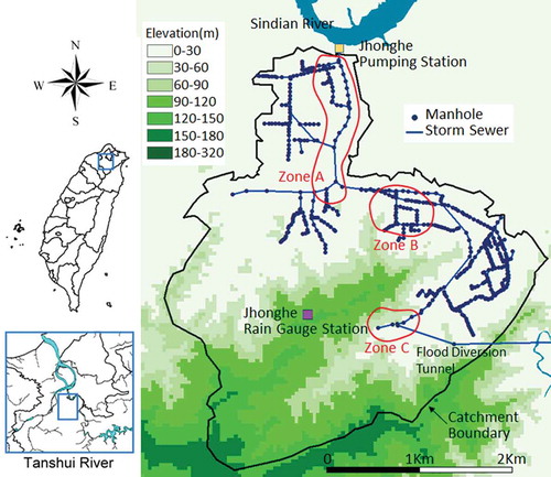
Figure 1. Topography of the study area.

Water-level measurements play a key role in the holistic information on urban drainage. By integrating relevant technologies, a practical flood warning system can be developed. However, a traditional wired water-level measurement system is costly due to its complex installation and its large scale (e.g. urban drainage). A regional wireless sensing network can be used to provide an affordable option for transmitting water-level measurements to a web-based system. To improve the response time for flood warnings, two warning water levels are set according to the rate of rising water level for larger drainage, and these levels can be used for possible flood warnings in the region. For smaller drainage, only one warning level is set due to its rapid water-rising rate.

Many studies reported in the literature have contributed to flood warning systems. The World Meteorological Organization (WMO 2011) defined 11 different kinds of floods, and the urban flood is one of them. Basically, there are two types of flood routing models, one is hydrological routing (lumped, distributed), and the other is hydraulic routing (kinematic wave, diffusion wave and dynamic wave). The dynamic, hydraulic routing is the most accurate but takes more time to complete simulation. Some flood warning systems combine the two kinds of models. It is stated that an urban flood warning is difficult due to the short response time of model simulations. The WMO (2011) has suggested that rainfall forecasting from radar and satellite images are potential technological options, and geographical information systems (GIS) are helpful in flood warnings. Besides displaying in GIS, the digital terrain model (DTM) is crucial in high-resolution modelling. Many river flood warning systems have been developed in many countries in recent years. Examples of warning systems used in China and Bangladesh are described below.

The China National Flood Forecasting System (CNFFS) has adopted a lot of models in different areas in China. The models include the Xinanjiang model (Zhao et al. 1980, Zhao 1992, Zhao and Liu 1995), the API model (Sittner et al. 1969), the Sacramento model (Burnash et al. 1973), the tank model (Sugawara 1995), the SMAR model (Tan and O’Connor 1996), the unit hydrograph method, and the synthetic constrained linear system (SCLS). Most of them are of the lumped type and are generally set as semi-distributed models (for example, the Sacramento and Xinanjiang models) to meet specific needs. The flood warning systems mentioned above are focused on large rivers, so the response time of the watershed is long.

The river flood warning system of Bangladesh has adopted a rainfall–runoff module (NAM, Nielsen and Hansen 1973) and a one-dimensional (1D) hydrodynamic module (MIKE11 HD, DHI 1999). The NAM predicts runoff and lateral flow that is inputted to MIKE11 HD for river routing. The quasi two-dimensional (2D) flow simulation on flood plains was realized by setting the flood plain as another river separate from the main river. The MIKE 21, 2D numerical, hydrodynamic model (DHI 2001) was used for storm surge simulation, and the phase and amplitude errors were corrected by minimizing an objective function based on real-time gauged data (Paudyal 2002).

Schmitt et al. (2004) combined the 1D drainage model and 2D street overland model for urban flooding simulations. Dey and Kamioka (2007) proved that the integrated simulations of the 1D river routing, 1D drainage model, and 2D overland model can more accurately simulate urban flooding. More recently, Shen et al. (2016) proposed a new rapid simplified inundation model (NRSIM) for simulation of floods induced by rainstorms in an urban area where data are scarce. The topography of each cell was simplified to a circular cone, and a mass conservation equation was used to simulate the water filling process. The spilling (flooding) process of each cell was calculated based on the characteristics of the cell and the surrounding ones. The concept model was then converted to a scenario for the US EPA Storm Water Management Model (SWMM) for simulation. In this way, simulation could be done very quickly on a large-scale, 30-m DEM, in 53.9 s for a total area of 92.3 km² with 102 573 cells.

Hong et al. (2016) combined an urban 2D-surface model, TREX, and a 1D-drainage model, CANOE, to form the TRENOE platform for urban storm water quantity and quality simulation. The TREX model is diffuse-wave based. The roofs of buildings are represented as virtual “sub-basins” in the CANOE model (nonlinear reservoir), and the 1D-Sewer Flow is kinematic-wave based (the other module in CANOE). This model was applied to a small urban catchment, Le Perreux sur Marne, which is near Paris (0.12 km²). The authors found that adequate numerical precision and accurate land-use data are crucial to water quantity modelling. In contrast, the high-resolution topographic data obtained using lidar and the variations in water flow parameters are not equally significant at a small urban catchment. It is doubtful that adequate numerical precision has such a huge impact on the simulation results. The above-mentioned literature refers to river flood warning or urban flood simulation systems focused mostly on how to improve the accuracy of model performance, such as the fitness of the water surface levels or discharges in either the rivers or urban drainage. No reports mentioned the trigger levels in an urban drainage flood warning system. The literature maintains that levels triggering urban floods are rare. Lee et al. (2013) proposed an assessment of sewer flooding based on an ensemble quantitative precipitation forecast in Taiwan. Data on the design capacities of the sewers were collected and the warning for urban flooding was set based on predicted resemble rainfall and design capacities. The spatial resolutions of flood warning systems are districts whose areas range from 5.71 to 321.13 km² (New Taipei City, Taiwan, for example). In short, they use rainfall for urban flood warnings.

To fill the gap in the research, this study mainly focuses on setting trigger levels in an urban drainage flood warning system. In order to evaluate the impact of flooding (inundation depth and area), the outflows from manholes to the ground surface are simulated by the 1D hydraulic computation model, SWMM (dynamic wave), and those results are used as sources for a self-developed, 2D diffusive overland flow model for urban flooding simulation.

An urban drain flood warning system with a wireless network has been tested during recent typhoon events in the study area and its applicability is proven. Through this affordable system, the real-time water level in urban drainage can be found. If the water reaches warning levels, measures can be taken for disaster reduction.

2 Study area

The Jhonghe urban drainage system is located in New Taipei City, Taiwan. The hills are in the southern part of the study area, and the Sindian River, a tributary of the Tamshui River, is in the northern part of the study area (as shown in Fig. 1). The catchment area of the Jhonghe urban drainage is 1324 ha, with a population of 413 676 (as of July 2017). The network includes 504 manholes and 23.65 km of pipes, in 499 sections, with diameter greater than 50 cm. The storm sewer system collects the runoff and drains into the Sindian River. A pumping station has been built downstream of the drainage network to pump the water out of the region when the river water level is too high to drain the runoff by gravity. All the detailed data for the drainage network, such as the elevations of all links and nodes, the storage capacities of the nodes, and the diameters of pipes, were obtained from the New Taipei City government. Three zones, namely Zone A, Zone B and Zone C, were chosen for installation of 14 water-level sensors, and five commercial water-level gauges were installed for verification of data from the water-level sensors. Zones B and C are located in the foothills where the elevation is about 200 m a.s.l. The study area is low-lying and is usually inundated when receiving torrential rains brought by typhoons. In 1996, Typhoon Herb created an inundation depth of 0.6–3.0 m in this area; in 2001, Typhoon Nari produced rainfall that caused an estimated inundation depth of 1.6 m in this area; and torrential rain in 2006 induced an inundation depth of 0.2 m. More recently, some regions were flooded due to Typhoon Jangmi in 2008. The Jhonghe pumping station is located at the end of the drainage system with a 20.0 m × 5.7 m forebay and a pumping capacity of 94.16 cm/s (Fig. 1). The land use in the study is shown in Figure 2. A flood diversion tunnel is connected to the drainage system in Zone C to divert the peak flow in this zone.

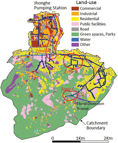
Figure 2. Land use of the study area.

3 Wireless sensor network

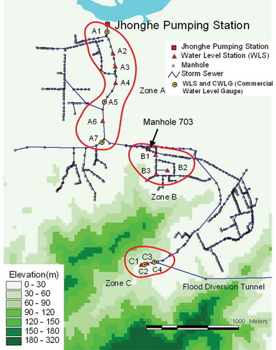
This study implements the integration of pressure sensors with a regional wireless sensing network for real-time monitoring of water levels. The wireless sensor network has been used in many fields (Lynch et al. 2006, Hoult et al. 2010, Chae et al. 2011). In order to observe the urban drainage water levels, 14 water-level stations (WLSs) equipped with pressure sensors were installed in the study area (Fig. 3). The system deploys three wireless local area sensing networks for the separate zones: Zone A (A1–A7), Zone B (B1–B3) and Zone C (C1–C4), as shown in Figure 3.

Figure 3. Layout of water-level stations (WLS) and wireless network in Jhonghe, Taipei.

This study selected a short-range wireless transmission protocol named ZigBee as the local transmitter network for transferring data gathered from the WLSs to local coordinator nodes. Local coordinator nodes transmit data to the database via the General Packet Radio Service (GPRS) network. The ZigBee protocol is IEEE 802.15.4 compliant and supports star, mesh and tree network topologies. Thus, the wireless sensing network (WSN) provides an option for a real-time wireless monitoring system for flood warning in urban drainage under a limited budget. Tree topology was selected as the network topology because it allows nodes to branch out from the network in many directions and best suits wide spreading bifurcations of the network. The long-distance transmission equipment selected for this study is GPRS due to its speed and efficiency across the mobile network. The local WSN connects to a remote database server which decodes the network’s raw packets and stores the decoded data. Furthermore, a monitoring website was constructed for remote users to access the real-time information and to acquire the data for post-processing.

In this study, the pressure-sensing element used in the WSN is a commercially available pressure sensor (LM Series) manufactured by Schaevitz® Sensors, suitable for water or gas pressure measurement. The sensor incorporates a stainless steel and plastic isolation suitable for level sensing in water. The water-level range in this study is set from 0 to 3.5 m. The operating temperature ranges from –30 to 85°C. The accuracy of the measured pressure is ±1%. In other words, for a water depth of 3.5 m, the error is less than 3.5 cm.

Before the sensor could be used in the field, the correlation curve of the output signal and the water surface level was calibrated in a water tank at the Hydrotech Research Institute, National Taiwan University. Each in situ WLS includes one calibrated pressure sensor mounted near the bottom of the conduit.

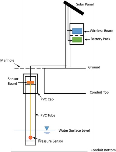
The power supply of the self-developed water-level meter derives from a 30-W solar panel which is connected to a 12-V battery pack. The sensor is wired to a self-developed sensor board which receives the output signal from the sensor. The sensor board is connected to the ZigBee Network module, which was made by the Institute for Information Industry, Taiwan. The board and sensor are protected by a PVC tube. The modules of the self-developed WLS are shown in Figure 4. The WLS transmits the data wirelessly to a web-based database, so the RAM of the transmission module is not large (96 kB). The sampling interval of the WLS measurements is normally 20 min for non-storm times, but it is adaptable to as high as 30 s during storm events. The transmission rate is the same as the sampling rate of the measurements. This is sufficient for the rate of the rising water levels.

Figure 4. Schematic diagram of a water-level station (WLS).

Commercial water-level gauges (CWLGs, model type: HOBO U20-001-0 manufactured by Onset Computer Co.) record water levels with data loggers. The operating temperature ranges from 0 to 40°C. The accuracy of the measured pressure is ±0.1%. This water-level gauge features high accuracy to measure pressure and temperature, and it has enough memory for the data logger. However, the data recorded inside a CWLG cannot be transmitted to the wireless network. The CWLG uses a built-in data logger for storing data. We need to manually upload the data from the data logger to a notebook on-site. When the storage of the CWLG’s data logger is full, the oldest data are overwritten. The CWLG does not have the capability for real-time data transmission. Therefore, these data collected by the CWLGs were used for comparison with those measured by the WLSs. In order to check the applicability of a WLS, the data from five CWLGs is used for the verification of the WLS. However, not all WLSs in this study were coupled with the commercial loggers due to the costly hardware.

The cost of LM sensors manufactured by Schaevitz® Sensors and the HOBO U20-001-01 made by the Onset Computer Co. is about US$150 and US$1000, respectively. The cost of a unit self-developed WLS (including pressure sensor, network module, solar panel, battery packs, PVC pipe, stainless box, shaft, etc.) is about US$1450. Other than the low cost of a WLS, advantages include: (a) sampling as requested – from a few min to 30 s per data; (b) no cables needed for transmission; and (c) real-time transmission to a web-based database. The disadvantages of a WLS include: (a) transmission distance limited to 200 m, so a relay station needs to be set up if the transmission distance is great than 200 m (a more powerful wireless module can be used for up to 500 m or more, but the power consumption of the 500 m module is greater than that of the 200 m one); (b) although it is powered by a solar panel, it may malfunction in bad weather, such as a period of cloudy days (a fixed line power supply is recommended, with the solar power used for a backup); (c) the pressure sensor may become blocked by bed debris; and (d) it provides less accuracy when compared to the commercial ones, but the error of a few centimetres is acceptable for flood warning.

4 Urban inundation model

Although sensors can obtain the real-time water level in a drainage system, they need a few past flood event water levels to set the warning water level. The WLSs do not provide sufficient data for setting flood warning water levels, so the 1D-SWMM model assists in generating the dataset needed. To evaluate the impacts of inundation zones and depths when water overflows the manholes, an overland 2D model is also integrated with the 1D-SWMM model.

The urban inundation model is divided into two successive processes, namely the drainage process and the inundation process. For the drainage process, the 1D hydraulic model SWMM is applied for the computation of flow in the storm drainage systems and outflow at the manholes. For the inundation process, a 2D diffusive overland flow model (2D-DOFM) is applied for surface runoff and inundation simulation (Hsu et al. 2000, 2002).

4.1 Storm water management model (SWMM)

The SWMM, developed under grants from the US EPA, is commonly applied to drainage systems in urbanized areas. The SWMM consists of several modules for analysis of different processes. Two of them, the RUNOFF and EXTRAN modules (Huber et al. 1984, Huber and Dickinson 1988, James et al. 2005) are widely used all over the world and thus were chosen for this study. The RUNOFF module performs a hydrological process simulation, and its outputs are used as inputs for the EXTRAN module, which computes the conduit flow in a storm drainage system using an explicit differencing scheme of Saint Venant equations. The geographic parameters of RUNOFF include the sub-catchment area, width, slope, roughness, etc., and it handles the computation of infiltration using the Horton equation.

The link–node concept is applied in the SWMM. Links represent the conduits in the drainage system, and nodes represent the manholes, junctions or outlets in the drainage system. Nodes function as storage elements. Before a sewer surcharge happens, the inflows and outflows of a node must equal the storage change during a given time step (i.e. ΣQ_t = ΔS_t/Δt) as depicted in Figure 5(a), where Q_t is all inflows and outflows at time t, and ΔS_t is the storage change during a given time step, Δt.

Figure 5. Mass conservation in the manhole for (a) sewer flow and (b) surcharge flow.

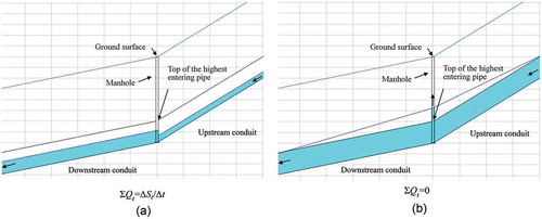
Sewer surcharges occur when discharge flows from pipes to a node where the water surface of the node lies in between the top of the highest entering pipe and the ground surface (Fig. 5(b)). In this situation, the continuity equation for each node equals zero (i.e. ΣQ_t = 0). Overflow (flooding) occurs when the sum of the pressure head and elevation head exceeds the ground surface, and water is released from the drainage to the ground surface.

The SWMM simulates hydraulic variables in the conduits; however, it cannot provide detailed information for flood warning, such as inundation zones and depths caused by overflow from the manholes. Thus, those overflows are treated as inputs for the 2D-DOFM for overland flow simulations.

4.2 The 2D diffusive overland flow model (2D-DOFM)

To evaluate the impacts of flooding (inundation zones and depths), the 2D-DOFM is used for inundation simulation. Assuming that the inertia term of the water flow on the urban surface is small compared to gravitation and friction terms, the inertia terms in the momentum equations are neglected. It has been found that the non-inertia flow is suitable for modelling of overland flow conditions (Akan and Yen 1981, Hromadka and Lai 1985, Fennema et al. 1994). The depth-averaged shallow-water equations, including the continuity Equation (1) and momentum Equations (2) and (3), can be simplified and written as:

(1)

(2)

(3)

where h is the depth of the overland flow, u is the velocity component in the x-direction, v is the velocity component in the y-direction, z is the ground surface elevation, t is time, g is gravitational acceleration, n_g is Manning’s roughness coefficient of the ground surface, and is the source or sink per unit area. The overflow calculated from SWMM is treated as a source in the 2D-DOFM. In the present study, a two-step alternating direction explicit (ADE) scheme is adopted. The finite difference equations are derived from Equations (1)–(3).

5 Model linkage, calibration and verification

The flowchart showing the linkage of the integrated model is shown in Figure 6. The SWMM includes the RUNOFF and EXTRAN modules. First, the RUNOFF block of SWMM uses the rainfall as input to calculate the surface runoff discharge hydrographs. The EXTRAN block of SWMM uses the surface runoff discharge as input at the manhole to calculate the conduit flow and calculates the hydrographs of the overflow flow rate at the manhole when the surface runoff exceeds the design capacity of the drainage system. The computation domain of SWMM covers the whole study area. The overflow hydrographs are subsequently used as sources imposed in the 2D diffusive overland flow model. The flood water does not re-enter manholes that are not surcharged. In short, the simulation results of the flooding are more conservative because the flood water may re-enter the drainage system.

Figure 6. Flowchart of the urban inundation model integration.

Calibration and verification of the SWMM were achieved by performing past events. Based on previous studies (Chang et al. 2013), Manning’s roughness coefficient n_c in the SWMM was first set according to the material of the drainage conduits, and then adjusted to fit the water-level measurement. The roughness coefficient, n_g, was set by the land-use type of the area (Fig. 2). Typhoon Aere (August 2004), Typhoon Haima (September 2004) and the torrential rain event (July 2006) resulted in floods involving the Jhonghe urban drainage system. The first two events were used for calibration of the SWMM, and the last event was used for verification of the SWMM at A5 (Fig. 7). Rainfall records from the central weather bureau’s raingauge stations in the Jhonghe area were employed for hydrological simulation in this study. The location of Jhonghe raingauge station is shown in Figure 1.

Figure 7. (a) Rainfall hydrographs and (b) survey and simulation water levels at A5 for (1) Typhoon Aere, (2) Typhoon Haima and (3) the 7 October 2006 torrential rain event.

For the 2D-DOFM, a 40-m DEM was used for modelling. The computational domain of the 2D-DOFM is for a DEM that is below the elevation of 50 m. Manning’s roughness coefficient n was also set based on land-use types: (i) 0.02 for roads; (ii) 0.08 for green land and parks; and (iii) 0.05 for built-up areas (commercial, industrial, residential and public facilities). It should be noted that when performing the simulations the operation rules of the Jhonghe Pumping Station and diversion discharge from the flood diversion tunnel were also taken into account.

5.1 Calibration

The maximum measurements of 10-min cumulative rainfall were, respectively, 8.5 and 16.5 mm (recorded at Jhonghe raingauge station) for Typhoon Aere (2004) and Typhoon Haima (2004). Rainfall hydrographs with peak intensities of 40.5 and 74.0 mm/h were recorded during these two events (Fig. 7(a-1) and (a-2)). Manning’s roughness coefficient, n_c, in the SWMM was first estimated from the material of the drainage pipes and then adjusted to fit the measured data from the CWLGs (HOBO U20-001-01; see Section 3). Figure 7(b-1) and (b-2) shows the simulation results from the water-level hydrograph measured at A5. Comparison of the simulation results and surveyed records of water levels reveals that water levels were properly simulated by the model in most conditions.

5.2 Verification

The maximum 10-min cumulative rainfall was 28.0 mm on 10 July 2006. A rainfall hydrograph with a peak intensity of 130.5 mm/h was recorded during this event (Fig. 7(a-3)). The value of n_c is the same as that used for calibration. The results from the simulated and measured water-level hydrographs at A5 are shown in Figure 7(b-3). Comparison of the simulation results and surveyed water-level records reveals that appropriate agreement is achieved. Simply stated, the SWMM is suitable for simulating the hydraulic characteristics of urban drainage in the study area. The calibrated and verified SWMM is used for setting the warning water levels described in later sections.

6 Results

6.1 Measured water levels

Fourteen WLSs have been installed in the study area and these are divided into three sensor network zones, A, B and C, according to the sub-catchments. Zone A includes seven WLSs (A1–A7); Zone B includes three WLSs (B1–B3); and Zone C includes four WLSs (C1–C4) (as shown in Fig. 3). In order to check the applicability of the WLSs, the data from five CWLGs (HOBO U20-001-01; see Section 3) were used for the verification of the WLSs. However, not all WLSs in this study are coupled with commercial loggers due to the costly hardware.

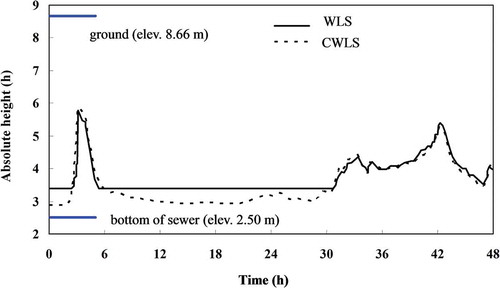
The measured water levels at A5 for WLS and CWLG when Typhoon Jangmi struck Taiwan between 26 and 29 September 2008 are shown in Figure 8. Figure 8 indicates the consistency of water-level measurements between WLS and CWLG (see Fig. 3 for locations). To reduce silting, the in situ pressure sensor of the WLS is placed 50 cm above the CWLG, which is mounted on the bottom of the drainage at this station. Thus, the horizontal line of the water level of the WLS in Figure 8 represents the elevation where the pressure sensor is installed.

Figure 8. Comparison of water levels measured by commercial water-level gauge (CWLG) and water-level station (WLS) at A5 during Typhoon Jangmi (2008).

6.2 Warning water level

For larger conduits, the warning water level relates to the rate of the rising water level and the response time for disaster reduction measures. The warning water level for a smaller conduit is defined later. For larger conduits, two stages of warning water levels are defined, as shown in Figure 9(b) and (a), respectively:

Figure 9. (a) Stage 2 warning water level (WL_s) and (b) Stage 1 warning water level (WL_o).

Stage 1 warning water level of an overflow:

(4)

Stage 2 warning water level of a surcharge flow:

(5)

where E_g is the ground surface elevation; E_c is the elevation of the top of the conduit; S_gi is the average rising rate of water level for overflow in the ith ΔT (subscript i is an integer index); S_ci is the average rising rate of water level for surcharge in the ith ΔT′, where ΔT and ΔT′ are the time steps for computation of S_gi and S_ci (both 10 min in this study).

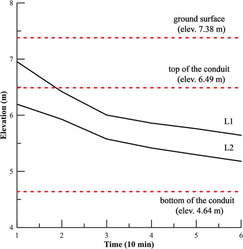
When the water level reaches WL_s, it will take T_s to reach the top elevation of the conduit, and when the water level reaches WL_o, it will take T_o to reach the ground surface (Fig. 9(a) and (b)). Manhole 703 (Fig. 3) is used for demonstrating WL_s and WL_o (Fig. 10). It should be noted that the sensor is not installed in Manhole 703 but the SWMM simulations are performed there. Thus, WL_o equals the ground surface elevation minus the summation of the average rising rate of water level times ΔT for i = 1 to n. The response time for disaster reduction action for WL_o is T_o = n × ΔT, where n = 3 for Manhole 703. In other words, the response time of WL_o: T_o = 30 min for n = 3 and ΔT = 10 min. Similarly, the response time for disaster reduction action for WL_s is T_s = n × ΔT′, where n = 3 for Manhole 703; i.e. T_s = 30 min for n = 3 and ΔT′ = 10 min. The reason for choosing n = 3 will be explained later.

Figure 10. Computation of rising rate of water surface at Manhole 703 during Typhoon Matsa (2005).

Because of the lack of past flood records, this study computes the rising rates of the water levels of historical events and the 5-year return period rainfall event by SWMM. In order to evaluate a suitable response time for disaster reduction measures, the time span of 60 min from the time the water surface reaches the ground surface or the top of the conduit is sliced into to six 10-min time steps. The rising rates of the water level in each 10-min time step are calculated. After computing all rising rates for different scenarios, the top three rising rates for each time step are averaged. The results are shown in Table 1, and the top three rising rates of water level are indicated by shaded cells. In Table 1, the water levels for some scenarios may not reach the ground surface and the rising rates may be negative due to the water level receding in a specific time step that results from the decrease in rainfall.

Table 1. Rising rate of warning water level in 60 min at Manhole 703. Shaded cells contain the top three water-level rising rates.

	Stage 2 rising rate of water level in 10 minutes (surcharge), Sci (m/h)						Stage 1 rising rate of water level in minutes (overflow), Sgi (m/h)
ith ΔT′ or ith ΔT	1	2	3	4	5	6	1	2	3	4	5	6
ΔT′ or ΔT	10 min	10 min	10 min	10 min	10 min	10 min	10 min	10 min	10 min	10 min	10 min	10 min
5-year-period design rainfall	0.12	0.12	0.18	0.12	0.12	0.06	0.60	0.54	0.30	0.36	0.54	0.60
Typhoon Matsa 3–6 August 2005	1.44	1.08	0.42	0.24	0.42	0.66	0.60	1.62	1.14	1.02	1.32	1.44
Typhoon Haitang 16–20 July 2005	0.18	0.18	0.24	0.24	0.24	0.18	–	–	–	–	–	–
Typhoon Haima 11–13 September 2004	1.32	0.60	0.00	▽	▽	▽	3.30	1.32	0.60	0.00	▽	▽
Typhoon Aere 23–26 August 2004	1.80	0.72	0.18	0.00	0.00	▽	3.60	1.80	0.66	0.12	0.06	0.06
Typhoon Nari 13–19 September 2001	0.24	0.54	0.78	0.96	0.96	0.48	0.06	3.42	3.06	0.54	▽	▽
Typhoon Xangsane 30 October–1 November 2000	0.42	0.60	0.72	0.78	0.54	0.18	0.12	2.58	1.74	1.02	0.42	0.60
Typhoon Babs 25–27 October 1998	0.36	0.36	0.36	0.42	0.66	0.96	–	–	–	–	–	–
Typhoon Zeb 13–17 October 1998	2.04	3.06	4.80	1.14	0.00	0.00	0.78	3.60	2.70	0.24	▽	▽
Typhoon Herb 29 July–1 August 1996	0.30	0.42	0.48	0.36	0.12	▽	–	–	–	–	–	–
Top 3 average	1.76	1.62	2.10	0.96	0.72	0.70	2.56	3.20	2.50	0.86	0.60	0.70

▽: Negative rising rate due to the water surface level falling.

-: Not applicable due to the water surface not reaching the ground surface.

Figure 10 shows the computation of the rising rate of water surface levels, S_gi and S_ci, at Manhole 703 during Typhoon Matsa (2005). The computation time step of the SWMM simulation is also 10 min. The simulated water surface may not be exactly the same as the elevation of the top of the conduit when computing the rising rates of S_c1 (as shown in the circle in Fig. 10). The nearest water level simulated by SWMM will be used for computing S_c1. The water surface overflows at the end of some simulation time steps so there is no error in computing S_gi.

Table 2 shows the rising rate of the water level at Manhole 703 for WL_s and WL_o in 60 min at each 10-min time step. The rising rates are also shown in Figure 11. The rising rates for S_ci and S_gi are higher for the first 30 min of the 60-min period than for the second 30 min. When the response time equals 30 min, the Stage 2 warning water level is about 50% of the full flow area of the conduit. If the response time is set too short (such as 10 min), it is not applicable for taking disaster reduction measures. However, if the response time is set too long (such as 60 min), it will trigger the Stage 2 warning water level too frequently due to its low warning elevation. Thus, for Manhole 703, we set both response times for the Stage 1 and 2 warning water levels to 30 min. For other manholes, the same procedure should be followed to set the response time for disaster reduction measures.

Table 2. First- and second-stage warning water levels (m) at 10-min time steps in a 60-min period at Manhole 703.

Response time (min)	10	20	30	40	50	60
Stage 2 level (m)	6.20	5.93	5.58	5.42	5.30	5.18
Stage 1 level (m)	6.95	6.42	6.00	5.86	5.76	5.64

Figure 11. Rising water surface rates at Manhole 703. L1: Stage 1 warning water level; L2: Stage 2 warning water level.

The water level simulated by SWMM at Manhole 703 for Typhoon Jangmi (2008) is shown in Figure 12. The results of the SWMM simulation show a horizontal line when water reaches the ground surface. The elevation of the top of the conduit is 6.44 m, and the ground surface elevation is 4.64 m. The warning levels for surcharge and overflow are 5.58 m (Stage 2 warning) and 6.00 m (Stage 1 warning). The rising time of the rainfall histogram matches that of the water level in the conduit. It can be seen that the rising water level in the conduit responds to the effects of rainfall very quickly due to the small catchment of the drainage system.

Figure 12. Simulated water level, Stage 1 (L1) and Stage 2 (L2) warning water levels of the SWMM during Typhoon Jangmi (2008) at Manhole 703.

Different associated reduction measures for the Stage 1 and 2 warning water levels are briefly described below. For the Stage 2 warning water level of a surcharge flow, WL_s is used for the following disaster reduction measures:

1. Mobile pump employment: Small-capacity mobile pumps can be employed in the possible flooding area to pump out flood water in the basements of buildings. Large-capacity mobile pumps can be used in the intake basin of the pumping stations to temporarily increase the original pumping capacity. At this stage, the flood-relief equipment can be transferred to the warning area.

2. Traffic control: During flooding, urban traffic can be heavily affected. Re-routing traffic is important when flooding occurs during rush hours. At this level, the work force of traffic control is employed in the area.

3. Flood warnings and related measures: The relevant authorities include local government (city government in this case), subway traffic controllers and agencies of emergency management, who should be informed and prepared for possible flooding. The announcements of possible flooding should be broadcast to the public on television or websites so that they can take proper flood prevention measures such as closing domestic floodgates, piling sandbags and avoiding travel around the possible flooded areas.

For the Stage 1 warning water level of the surcharge flow, WL_o is used for the following disaster reduction measures:

1. Mobile pump employment: the equipment should be positioned to function.

2. Traffic control: personnel should be positioned to prevent vehicles and pedestrians from trespassing and redirect them to alternative routes.

3. Flood warnings and related measures: The flood prevention measures of related authorities should take action at this time. Evacuation facilities, such as rubber boats and rescue vehicles, should be ready. Announcements of flooding broadcast by local police and the heads of neighbourhoods are recommended. The authorities should finish the above-mentioned measures during the first-stage warning water level and caution the public for evacuation.

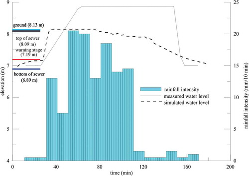
In Taiwan, many manholes of the smaller drainage systems have very shallow depths between the ground surface and the tops of the conduits, and B2 in Zone B is such a case. Since the water takes a very short time to rise from the top of the conduit to the ground surface, only one warning water level is suitable for warning purposes, as depicted in Figure 13. To distinguish it from the Stage 1 and 2 warning water levels, the warning water level of this kind of manhole is denoted as WL_n.

Figure 13. Calculation of warning water level for a shallow-depth manhole.

By definition, WL_n is equal to the ground surface elevation minus the summation of the average rising rate of water level times ΔT for i = 1 to n. For example, the response time of B2 for disaster reduction action for WL_n is T_n = n × ΔT, where n = 2, i.e. T_n = 20 min for n = 2 and ΔT = 10 min. Following the same procedure as for the Stage 1 and 2 warning water levels for larger conduits, the rising rate of water surface level S_ni is defined as the average rising rate of water level for overflow of a narrow-depth manhole in the ith increment of ΔT. Table 3 shows the S_ni for different scenarios, and the top three average rising rates are also indicated. Table 4 shows the computed warning water level based on the results in Table 3. The response time before the water overflows the manhole is set to 20 min for two main reasons: (a) 10 min is too short a time to take disaster reduction measures; and (b) the warning level computed for 30 min is 7.07 m, which is too near the bottom of the conduit (elevation: 6.89 m). Thus, a 20-min response time is selected for the warning water level at B2.

Table 3. Rising rate of warning water level for ΔT = 10 min in a 60-min period at B2. Shaded cells contain the top three water-level rising rates.

ith increment of ΔT	Rising rate of water level in 10 min (overflow), Sn (m/h)
	1	2	3	4	5	6
5-year-period design rainfall	0.3	▽	0.42	0.42	1.14	0.78
Typhoon Matsa 3–6 August 2005	2.88	2.4	0.66	0.00	0.00	0.06
Typhoon Haitang 16–20 July 2005	–	–	–	–	–	–
Typhoon Haima 11–13 September 2004	0.54	1.44	1.08	1.08	0.36	0.00
Typhoon Aere 23–26 August 2004	1.44	1.62	0.36	0.06	0.00	0.00
Typhoon Nari 13–19 September 2001	2.40	3.60	0.24	0.60	0.00	0.00
Typhoon Xangsane 30 October–1 November 2000	–	–	–	–	–	–
Typhoon Babs 25–27 October 1998	–	–	–	–	–	–
Typhoon Zeb 13–17 October 1998	3.42	2.46	0.30	0.66	▽	0.00
Typhoon Herb 29 July–1 August 1996	–	–	–	–	–	–
Top 3 average	2.58	2.82	0.72	0.78	0.50	0.28

▽: Negative rising rate due to the water surface level falling.

-: Not applicable due to the water surface not reaching the ground surface.

Table 4. Warning water level in 60 min at B2.

Response time (min)	10	20	30	40	50	60
Time step (min)	10	10	10	10	10	10
Warning level of the shallow-depth manhole (m)	7.66	7.19	7.07	6.94	–	–

-: Not applicable (warning water surface level is below the bottom of the conduit).

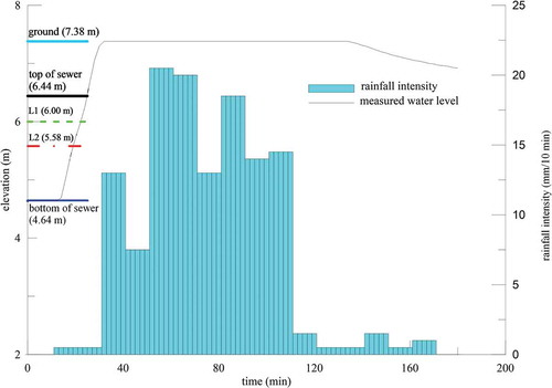
The water level simulated by SWMM and that of the WLS at B2 during Typhoon Jangmi is shown in Figure 14. The patterns of the measured and simulated water levels are similar. The rising rate of the water level simulated by SWMM is faster than that of the WLS measurement. The result of the SWMM simulation shows a horizontal line when water reaches the ground surface. The elevation of the top of the conduit is 8.09 m and the ground surface elevation is 8.13 m. It is suitable to assign only one warning water level for this kind of conduit. The warning level for overflow is 7.19 m. The higher water surface level of WLS than the simulated level indicates that flooding occurred during this event. The sensor can detect the flooding above the manhole, and the flooding depth just above the manhole is about 0.7 m in this event. Before Typhoon Jangmi’s landfall (2008), a flood incident around B2 was reported on the news with an inundation depth of about 0.5 m (Wu et al. 2008).

Figure 14. Measured water level of WLS, simulated water level of the SWMM, Stage 1 (L1) and Stage 2 (L2) warning water levels during Typhoon Jangmi (2008) at B2.

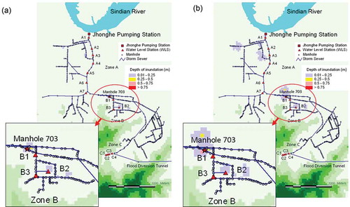
In Figure 15, the overflows from the manholes in the system are used as source terms in the 2D-DOFM for flood simulation. In Figure 15(a), the most inundated area is Zone B where B2, Manhole 703 and a few manholes to the right of B2 are also flooded after the water level reaches the first-stage warning level for 20 min. At 60 min from the simulation time of Figure 15(a), the inundated areas of Zone A and Zone B enlarge and can be seen in Figure 15(b). By this analysis, some critical points are identified, and for those hotspots it is recommended that an increase in the drain capacity be made or sensors be installed for flood warning in the future. In addition, the flood diversion tunnel is proven to be effective in reducing the possible flooding in Zone C that occurred before its installation.

Figure 15. Inundation depths for (a) 20 min and (b) 80 min after the water level reaches the Stage 1 warning water level (L1) during Typhoon Jangmi at B2.

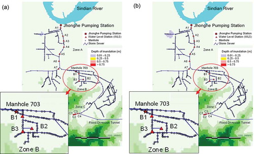
In addition to inundation depth maps for Typhoon Jangmi (2008), the inundation depth maps for the 5-year return period rainfall (typical design code for the urban storm drainage in Taiwan) are performed to evaluate the possible impacts of flooding. The inundation depths for 20 and 80 min after the water level reaches the Stage 1 warning water level are shown in Figure 16. The cumulative rainfall for the 5-year return period rainfall is less than that of Typhoon Jangmi. It can be seen that B2 is not flooded in both Figure 16(a) and 16(b). The information on depth and area of possible flooding can be used for deploying facilities and personnel in advance for disaster reduction measures and future drainage system improvement.

Figure 16. Inundation depths for (a) 20 min and (b) 80 min after the water level reaches the Stage 1 warning water level (L1) of the 5-year design rainfall.

6.3 Process of flood warning

The flowchart of the whole system is shown in Figure 17. Authorities can access the real-time water-level data collected by in situ pressure sensors, and the data are transmitted by GPRS to a web-based system. The staff of the Water Resource Bureau of New Taipei City monitor the warning levels on the web page. When the water level exceeds the warning levels, the manholes with possible flooding will automatically be highlighted for notification to the users on the system. An SMS (Short Message Service) message of flood warning can be sent to the affected residents, and mobile pumps can be deployed to areas that may be flooded.

Figure 17. Flowchart of the wireless real-time flood warning system.

As the two warning water levels are set, authorities can take disaster reduction measures when the water level reaches these levels. In the flowchart, related disaster reduction measures are also listed for reference. When there is only one warning water level (such as for B2), the disaster reduction measures should be taken quickly.

The water level at Manhole 703 reached the ground surface (elevation: 7.38 m) from the Stage 1 warning water level in about 20 min during Typhoon Jangmi (2008) due to its large total cumulative rainfall and high rainfall intensity. In this event, the actual response time for disaster reduction measures is 20 min, which is shorter than the response time of 30 min estimated by the analysis of rising water rates from past events.

Although a real-time flood warning system could successfully provide storm drainage water-level information for warning purposes, there is still a lot of variation in the rising rate of water levels. The real-time water levels of the follow-up hydrological events can be used for estimating the rising rates of the water level instead of SWMM simulation results. This wireless real-time monitoring system for flood warning in urban drainage performed very well compared to commercial ones. In addition, this system is economical and reliable, which makes large-scale WLS installations possible. The monitoring network can provide essential water-level information for taking disaster reduction measures.

7 Conclusions

This paper illustrates the successful integration of pressure sensors and a tree-type WRN for constructing a regional wireless sensing network to acquire real-time water levels of storm drainage. In this study, the short-range wireless transmission protocol ZigBee is used. All water-level data in the network are transmitted to a web-based system by a GPRS network. The water-level measuring system is feasible in the field and is applied in the case study. The comparison of water-level measurements between the WLSs and the CWLGs shows they agree very well. In other words, the newly developed WLSs work properly, as do the CWLGs. Due to the low cost of the WLSs, they are suitable for large-scale water-level monitoring of urban drainage in the future. To assure accuracy, CWLSs are also recommended to be installed in selected locations for comparison.

After acquiring reliable water-level data, authorities need the warning water level in order to take disaster reduction measures. The two stages of warning water levels are defined for larger conduits in this study. Due to the lack of past drainage water-level data, the warning water level is estimated by performing the SWMM (1D drainage model) for past rainfall events. The second stage is defined as the water level that will reach the top of the conduit in the response time, T_s. When the water level reaches the second stage, the water in the conduit begins to surcharge the manhole. The first stage is defined as the water level that will reach the ground surface in the response time T_o. Two response times (T_o and T_s) are used for taking disaster reduction measures such as flood warning and traffic control. In practice, the Stage 1 warning water level is calculated by the ground surface elevation minus the summation of the average rising rate of the water surface level (S_gi) times the time step ΔT_i (i = 1 to n where n needs to be determined), where S_gi is the average rising rate of water surface level at the ith time step. The Stage 2 warning water level is calculated in a similar manner. The rising rates of the water surface level are estimated from the simulation of past events by the 1D hydraulic model, SWMM, due to limited historical data. The response times T_o and T_s are decided by analysing the rising rates of the water level in the conduit for different scenarios. In order to avoid inadequate time for taking disaster reduction measures or the possibility of triggering the warning water level too frequently, the response times for the first- and second-stage warning water levels are both set at 30 min. For smaller drainage system conduits, only one warning water-level stage is needed due to the smaller diameter. One example of the warning water levels of the smaller conduits is described in this paper.

In order to evaluate the impacts of urban flooding, the integrated SWMM and 2D overland flow model (2D-DOFM) is applied to construct the potential inundation maps. In this way, the impacts when water surcharges the manhole can be evaluated. With hotspots of possible flooding available, corresponding measures can be taken. The flow can surcharge from the manholes in the integrated model, but the flood water cannot re-enter the manholes. In the future, it is recommended to rewrite the interchange mechanism between the overland flow and drainage flow for better representation of real flood events.

Therefore, the flood warning system can provide reliable water-level information for disaster reduction measures, and the possible impact area of flooding can also be estimated from the potential inundation map. Simply stated, this system can help authorities construct a flood warning system under a limited budget and inform the people in the inundation-prone areas to help prevent extensive damage, and the methodology established can be widely applied in setting warning stages for urban flooding.

Acknowledgements

The authors thank the Hydrotech Research Institute of the National Taiwan University and the National Center for Research on Earthquake Engineering for use of their facilities and technical support.

Disclosure statement

No potential conflict of interest was reported by the authors.

Additional information

Funding

This study was partially financially supported by the Water Resource Bureau, New Taipei City, Taiwan and by the Ministry of Science and Technology, Taiwan [Grant no. NSC96-2111-M-002-002, NSC96-2111-M-002-003], and by the National Taiwan University Excellence Research Program [95R0066-BE03-03].

References

- Akan, A.O. and Yen, B.C., 1981. Diffusion-wave flood routing in channel networks. Journal of the Hydraulics Division of ASCE, 107 (6), 719–732.
- Burnash, R.J.C., Ferral, R.L., and McGuire, R.A., 1973. A generalized streamflow simulation system: conceptual modeling for digital computers, technical report. Sacramento, CA: Joint Federal and State River Forecast Center, US National Weather Service and California Department of Water Resources.
- Chae, M.J., et al., 2011. Development of a wireless sensor network system for suspension bridge health monitoring. Automation in Construction, 21, 237–252. doi:10.1016/j.autcon.2011.06.008
- Chang, H.K., et al., 2013. Improvement of drainage system for flood management with assessment of climate change effects. Hydrological Sciences Journal, 58 (8), 1581–1597. doi:10.1080/02626667.2013.836276
- Cheng, S.J., Hsieh, H.H., and Wang, Y.M., 2007. Geostatistical interpolation of space-time rainfall on Tamshui River Basin, Taiwan. Hydrological Processes, 21 (23), 3136–3145. doi:10.1002/hyp.6535
- Dey, A.K. and Kamioka, S., 2007. An integrated modelling approach to predict flooding on urban basin. Water Science & Technology, 55 (4), 19–29. doi:10.2166/wst.2007.091
- DHI (Danish Hydraulic Institute), 1999. Manual: MIKE 11 flood forecasting model. Hørsholm, Denmark: DHI.
- DHI (Danish Hydraulic Institute), 2001. MIKE21 coastal hydraulics and oceanography hydrodynamic module. Reference manual. Hørsholm, Denmark: DHI Water & Environment.
- Fennema, R.J., et al., 1994. A computer model to simulate natural everglades hydrology. In: S.M. Davis and J.C. Ogden, eds. Everglades, the ecosystem and its restoration. Boca Raton, FL: St. Lucie Press, 249–289.
- Hong, Y., Bonhomme, C., and Chebbo, G., 2016. Development and assessment of the physically-based 2D/1D model “TRENOE” for urban stormwater quantity and quality modelling. Water, 8 (12), 606. doi:10.3390/w8120606
- Hoult, N.A., et al., 2010. Long-term wireless structural health monitoring of the Ferriby road bridge. Journal of Bridge Engineering, 15 (2), 153–159. doi:10.1061/(ASCE)BE.1943-5592.0000049
- Hromadka II, T.V. and Lai, C., 1985. Solving the two-dimensional diffusion flow model. In: W.R. Waldrop, ed. Hydraulics and hydrology in the small computer age (Proceedings of the Specialty Conference, 12–17 August 1985, Lake Buena Vista, FL). New York, NY: American Society of Civil Engineers, 555–562.
- Hsu, M.H., Chen, S.H., and Chang, T.J., 2000. Inundation simulation for urban drainage basin with storm drainage system. Journal of Hydrology, 234, 21–37. doi:10.1016/S0022-1694(00)00237-7.
- Hsu, M.H., Chen, S.H., and Chang, T.J., 2002. Dynamic inundation simulation of storm water interaction between drainage system and overland flows. Journal of the Chinese Institute of Engineers, 25 (2), 171–177. doi:10.1080/02533839.2002.9670691
- Huber, W.C., et al., 1984. Storm water management model user’s manual version III. Cincinnati, OH: US Environmental Protection Agency.
- Huber, W.C. and Dickinson, R.E., 1988. Storm water management model user’s manual version IV. Athens, GA: US Environmental Protection Agency.
- James, W., et al., 2005. Water systems models user’s guide to SWMM. 381–396 Ontario:CHI.
- Lee, C.H., et al., 2013. Assessment of sewer flooding model based on ensemble quantitative precipitation forecast. Journal of Hydrology, 506, 101–113. doi:10.16/j.jhydrol.2012.09.053
- Lynch, J.P., et al., 2006. Performance monitoring of the Geumdang bridge using a dense network of high-resolution wireless sensors. Smart Materials and Structures, 15 (6), 1561–1575. doi:10.1088/0964-1726/15/6/008
- Nielsen, S.A. and Hansen, E., 1973. Numerical simulation of the rainfall–runoff process on a daily basis. Nordic Hydrology, 4, 171–190.
- NOAA (National Oceanic and Atmospheric Administration), 1997. Automated local flood warning systems handbook, weather service hydrology handbook no. 2. Washington, DC: Government Printing Office.
- Paudyal, G.N., 2002. Forecasting and warning of water-related disasters in a complex hydraulic setting-the case of Bangladesh. Hydrological Sciences Journal, 47 (S), S5–S18. doi:10.1080/0262666020949301
- Schmitt, T.G., Thomas, M., and Ettrich, N., 2004. Analysis and modeling of flooding in urban drainage systems. Journal of Hydrology, 299, 300–311. doi:10.1016/S0022-1694(04)00374-9.
- Shen, J., et al., 2016. A new rapid simplified model for urban rainstorm inundation with low data requirements. Water, 8 (11), 512. doi:10.3390/w8110512
- Sittner, W.T., Schauss, C.E., and Monro, J.C., 1969. Continuous hydrograph synthesis with an API-type hydrologic model. Water Resources Research, 5 (5), 1007–1022. doi:10.1029/WR005i005p01007
- Sugawara, M., 1995. Tank model. In: V.P. Singh, ed. Computer models of watershed hydrology. Littleton, CO: Water Resources Publications.
- Tan, B.Q. and O’Connor, K.M., 1996. Application of an empirical infiltration equation in the SMAR conceptual model. Journal of Hydrology, 185, 275–295. doi:10.1016/0022-1694(95)02993-1.
- WMO (World Meteorological Organization), 2011. Manual on flood forecasting and warning. Geneva, Switzerland: WMO, No. 1072.
- WRA (Water Resources Agency), 2001. Flood report of Tamshui River due to Typhoon Nari. Taipei, Taiwan: Water Resources Agency, Ministry of Economic Affairs.
- WRA (Water Resources Agency). 2008. Hydrological year book of Taiwan, Republic of China, 2007, Part I-Rainfall. Taipei, Taiwan: Water Resources Agency, Ministry of Economic Affairs, 5–7.
- Wu, Z.J., et al., 2008. Floods in Jhonghe, Yonghe, and Wenshan before Typhoon Jangmi’s landfall. [online]. Liberty Times Net. Available from: http://news.ltn.com.tw/news/local/paper/246388 [ Accessed August 2017].
- Zhao, R.J., et al., 1980. The Xinanjiang model. In: Hydrological Forecasting: proceedings of the Oxford Symposium, 15–18 April 1980. Oxford. Wallingford, UK: International Association of Hydrological Sciences,, IAHS Publ.129.
- Zhao, R.J., 1992. The Xinanjiang model applied in China. Journal of Hydrology, 135, 371–381. doi:10.1016/0022-1694(92)90096-E.
- Zhao, R.J. and Liu, X.R., 1995. The Xinanjiang model. In: V.P. Singh, ed. Computer models of watershed hydrology. Colorado: Water Resources Publications.