Hydrological uncertainty processor based on a copula function

ABSTRACT

Quantifying the uncertainty in hydrological forecasting is valuable for water resources management and decision-making processes. The hydrological uncertainty processor (HUP) can quantify hydrological uncertainty and produce probabilistic forecasts under the hypothesis that there is no input uncertainty. This study proposes a HUP based on a copula function, in which the prior density and likelihood function are explicitly expressed, and the posterior density and distribution obtained using Monte Carlo sampling. The copula-based HUP was applied to the Three Gorges Reservoir, and compared with the meta-Gaussian HUP. The Nash-Sutcliffe efficiency and relative error were used as evaluation criteria for deterministic forecasts, while predictive QQ plot, reliability, resolution and continuous rank probability score (CRPS) were used for probabilistic forecasts. The results show that the proposed copula-based HUP is comparable to the meta-Gaussian HUP in terms of the posterior median forecasts, and that its probabilistic forecasts have slightly higher reliability and lower resolution compared to the meta-Gaussian HUP. Based on the CRPS, both HUPs were found superior to deterministic forecasts, highlighting the effectiveness of probabilistic forecasts, with the copula-based HUP marginally better than the meta-Gaussian HUP.

KEYWORDS:

• hydrological forecasting
• uncertainty analysis
• probabilistic forecasts
• copula function
• Three Gorges Reservoir

Editor D. Koutsoyiannis Associate editor E. Gargouri

1 Introduction

Hydrological forecasting is a crucial non-structural flood mitigation measure and provides an essential basis for flood warning, flood control and reservoir operation (Guo et al. 2004, Calvo and Savi 2009, Chen et al. 2014c, Zhang et al. 2015). The forecasting models that are widely used at present are typically deterministic and model outputs are provided to users in the form of deterministic values (Chen and Yu 2007, Coccia and Todini 2011, Ma et al. 2013, Bergstrand et al. 2014, Li et al. 2014). However, a hydrological forecasting model is only a simulation of the real hydrological processes and is therefore imperfect and not precise (Ravines et al. 2008, Wetterhall et al. 2013). These models accept hydrological input, meteorological input, etc., and utilize conceptualized model parameters; these complex factors inevitably cause uncertainties in the hydrological forecasts (Freer et al. 1996, Montanari 2007, Montanari and Grossi 2008, Renard et al. 2010, Chen et al. 2014a). The principle of rational decision making under uncertainty indicates that when a deterministic forecast turns out to be wrong, the consequences will probably be worse than a situation where no forecast is available (Krzysztofowicz 1999, Verkade and Werner 2011, Ramos et al. 2013, Wetterhall et al. 2013). A rational decision maker who wants to make optimal decisions should therefore take forecast uncertainty explicitly into account (Berger 1985, Verkade and Werner 2011, Ramos et al. 2013). Therefore, quantitative assessment of inherent uncertainty is a critical issue. Hydrological forecasting services are trending toward providing users with probabilistic forecasts, in place of traditional deterministic forecasts.

The transition from a deterministic forecast to a probabilistic forecast is based on quantification of the uncertainty inherent in the deterministic forecast. The Bayesian Forecasting System (BFS) proposed by Krzysztofowicz (1999) provides a general framework to produce probabilistic forecasts via any deterministic hydrological model. Various probabilistic forecasting systems suited to different purposes have been developed within this framework (Reggiani and Weerts 2008, Calvo and Savi 2009, Biondi et al. 2010, Weerts et al. 2011, Sikorska et al. 2012, Pokhrel et al. 2013).

In the BFS, the total uncertainty is decomposed into input uncertainty and hydrological uncertainty. The hydrological uncertainty processor (HUP) is a component of the BFS that quantifies the hydrological uncertainty and produces a probabilistic forecast under the hypothesis that there is no input uncertainty (Krzysztofowicz and Kelly 2000). Through Bayes’ theorem, the HUP combines a prior distribution, which describes the natural uncertainty about the realization of a hydrological process, with a likelihood function that quantifies the uncertainty in model forecasts, and outputs a posterior distribution, conditional upon the deterministic forecasts. This posterior distribution provides a complete characterization of uncertainty, including quantiles, prediction intervals and probabilities of exceedence for specified thresholds, which are needed by rational decision makers and information providers who want to extract forecast products for their customers.

The HUP can be implemented in many ways, as different mathematical models for the prior distribution and likelihood function can be developed. Krzysztofowicz and Kelly (2000) introduced a meta-Gaussian HUP, which was developed on the basis of converting both original observations and model forecasts into a Gaussian space by using the normal quantile transform (NQT). This meta-Gaussian HUP has been used widely by many researchers in the fields of hydrology and meteorology (Chen and Yu 2007, Biondi et al. 2010, Biondi and De Luca 2013, Chen et al. 2013a).

Actually, the prior density and likelihood function are conditional probability distributions. It is well known that copula functions have outstanding capability to model joint distributions and give flexibility in choosing an arbitrary marginal distribution (e.g. non-Gaussian form), nonlinear and heteroscedastic dependence structure. The conditional probability distribution can be expressed in explicit form using a copula function (Favre et al. 2004, Nelsen 2006, Zhang and Singh 2006, 2007a, 2007b, 2007c, Genest and Favre 2007, Bárdossy and Li 2008, Chen et al. 2010, Zhang et al. 2011, 2013, 2012). These advantageous characteristics of a copula function motivated us to develop the prior distribution and likelihood function models in the original space directly, without a data transformation procedure into Gaussian space. The main objective of this paper is to propose a post-processor based on a copula function for a deterministic forecast model to produce probabilistic forecasts within the general framework of the HUP.

The remainder of this paper is organized as follows: the methodology is outlined and presented in Section 2; Section 3 introduces a case study of probabilistic inflow forecasts for the Three Gorges Reservoir (TGR) in China; the results and discussion are included in Section 4; and Section 5 draws the main conclusions of the work.

2 Methodologies

2.1 Hydrological uncertainty processor

Let predictand H be the observed discharge whose realization h is being forecast. Let estimator S be the output discharge generated by a corresponding deterministic forecast model whose realization s constitutes a point estimate of H. Let random variable H₀ represent the observed discharge at the time n = 0 when the forecast is prepared; then H_n (n = 1, 2, …, N) is the observed discharge at lead time n, and S_n (n = 1, 2, …, N) is the corresponding deterministic forecast discharge at lead time n. What the rational decision maker then needs is not a single number s_n, but the distribution function of predictand H_n, conditional on H₀ = h₀ and S_n = s_n. The purpose of the HUP is to supply such a conditional distribution function through Bayesian revision (Liu et al. 2016).

The posterior density function of predictand H_n, conditional on S_n = s_n and H₀ = h₀, is derived via Bayes’ theorem (Krzysztofowicz and Kelly 2000):

(1)

In concept, Bayes’ theorem revises the prior density function, which characterizes the prior uncertainty about H_n given H₀ = h₀. The extent of the revision is determined by the likelihood function, which characterizes the degree to which S_n = s_n reduces the uncertainty about H_n. The result of this revision is the posterior density function , which quantifies the uncertainty about H_n that remains after the deterministic forecast model generates forecast S_n = s_n.

2.2 Meta-Gaussian HUP

The structure of Equation (1) indicates that the posterior density strongly relies on both the prior density function and the likelihood function. At present, the most commonly used technique to construct the prior density and likelihood functions is the meta-Gaussian model, which involves three steps. First, both actual flow H_n and predicted flow S_n are converted into Gaussian space by employing the NQT method (Bogner et al. 2012). Second, the transformed and series are assumed to be linear and normally distributed. Finally, the posterior density function of H_n in the transformed Gaussian space is derived by linear regression, from which the posterior density of H_n in the original space can be found based on the Jacobian inverse transformation. For more detailed descriptions and mathematical formulations of the meta-Gaussian HUP, readers are referred to Krzysztofowicz and Kelly (2000) or Liu et al. (2016).

2.3 Copula-based HUP

Copula functions are an effective tool used to develop prior distribution and likelihood function models, in which the predictand and the deterministic forecast are allowed to have distribution functions of any form, along with nonlinear and heteroscedastic dependence structure. Therefore, they can be implemented in the original space directly without a data transformation procedure into Gaussian space.

2.3.1 Copula theory

A copula function connects multivariate probability distributions to their one-dimensional marginal distributions (Nelsen 2006). Let () be the cumulative distribution function (cdf) of X_i. The multivariate distribution can be expressed in terms of its marginal and the associated dependence function using Sklar’s theorem:

(2)

where C, the copula function, captures the essential features of the dependence among the random variables. A more detailed description of copula function properties can be found in Favre et al. (2004), Nelsen (2006) and Zhang et al. (2013).

2.3.2 Prior density

The prior cdf of H_n given H₀ = h₀ can be expressed as:

(3)

where is the conditional cdf, and P is the non-exceedence probability.

The prior density function is the corresponding probability density function (pdf) of and can be defined as:

(4)

Let H₀ and H_n be random variables with marginal cdfs, and . Then, U₁ and U₂ are uniformly distributed random variables; u₁ denotes a specific value of U₁, and u₂ denotes a specific value of U₂. Using the copula function, the joint cdf is expressed by .

Using the copula function, the conditional cdf and pdf can be rewritten as (Zhang and Singh 2006):

(5)

(6)

where is the density function of , and ; is the pdf of H_n. Equation (6) is the expression of the prior pdf.

2.3.3 Likelihood function

It is considered that S_n is a random variable with marginal cdf and pdf . The conditional cdf of S_n given H₀ = h₀ and H_n = h_n can be expressed as:

(7)

where is the conditional cdf.

The corresponding pdf of is defined as:

(8)

Using the copula function, the joint cdf of H₀, H_n and S_n, denoted as, can be expressed as . So the conditional cdf and pdf are rewritten as (Zhang and Singh 2007c):

(9)

(10)

where is the density function of . From another point of view, given H₀ = h₀ and S_n = s_n, the likelihood function of H_n can be calculated using Equation (10).

2.3.4 Posterior density

Substituting the Equations (6) and (10) into Equation (1), the pdf of H_n can be rewritten as:

(11)

For fixed realizations H₀ = h₀ and S_n = s_n, u₁ and u₃ are constants, while u₂ varies from 0 to 1. Since the denominator cannot be obtained directly by an analytic method, the Monte Carlo sampling technique (Xiong et al. 2014, Yu et al. 2014) is applied by the following steps:

1. Generate M random numbers u₂ from uniform distribution U(0, 1);

2. Compute the value of ;

3. Calculate the mean of the M calculated values, which is approximately equal to the definite integral (Kroese et al. 2013, Robert and Casella 2013).

Subsequently, the pdf can also be estimated.

2.4 Candidate marginal distributions and trivariate copulas

Specifying and determining marginal distributions of the actual flow H₀, H_n and predicted flow S_n (n = 1, 2, …, N) is an essential step. The actual flows {H_n: n = 0, 1, …, N} are considered as random variables. Given only such a record, there is usually no basis for assigning a probability distribution to flow H_n that differs from the distribution assigned to flow H₀, for any n = 1, 2, …, N within a few days. In other words, there is no a statistical difference between these 1 + N flow series (Koutsoyiannis and Montanari 2015). Therefore, we hold the opinion that the variables H_n follow the same marginal cumulative distribution functions (cdf) with H₀, and thus only the cdf of H₀ needed to be fitted. The predicted flows {S_n: n = 1, …, N} are considered as different random variables and different cdfs needed to be fitted for variable S_n.

The main purpose of this study is not hydrological frequency analysis, which aims to extrapolate the extreme events far beyond the observations (very low probabilities, e.g. return period exceeds 1000 years). Instead, the probability distribution of daily flows used in this paper refers to the flow–duration curve, which gives a summary of flow variability at a site and is interpreted as a relationship between any discharge value and the percentage of time that this discharge is equalled or exceeded during a given period (Vogel and Fennessey 1994, Castellarin et al. 2004, Shao et al. 2009). The flow–duration curve has been widely used by engineers and hydrologists around the world in numerous applications, such as hydropower generation, inflow forecasting, and designing of irrigation systems (Vogel and Fennessey 1995, Yokoo and Sivapalan 2011, Gottschalk et al. 2013).

In our study, we concentrated on the daily flow–duration curve. If the daily streamflow is assumed to be a random variable, the flow–duration curve may also be viewed as the complement of the cumulative distribution function used in hydrological frequency analysis when identifying the percentage of time with probability (Castellarin et al. 2004). As a consequence, the flow–duration curve is also a very practical tool used to describe hydrological regimes and represents the relationship between magnitude and frequency of flow (Vogel and Fennessey 1995, Liucci et al. 2014, Xiong et al. 2015).

Six commonly used distributions in hydrology, namely normal, gamma, Gumbel, Pearson type III, log-normal and log-Weibull, were selected as candidate models for H₀ and S_n (n = 1, 2, …, N). These univariate probability distributions are summarized in Table 1. In this study, the distribution parameters were estimated by L-moments method (Hosking 1990, Liu et al. 2017). The Kolmogorov-Smirnov (K-S) test statistic, D, was adopted to measure the goodness of fit between the candidate theoretical distribution and the empirical distribution (Tsai et al. 2001, Rahman et al. 2010). The 5% significance level was selected to reject or accept a fitted distribution, and then the probability distribution that provides the minimum D value was chosen as the best fitting distribution.

Table 1. Candidate univariate distributions adopted in this study.

Distribution	Probability distribution function (pdf)	Range
Normal
Gamma
Gumbel
Pearson type III
Log-normal	,
Log-Weibull

Different families of copulas have been described by Nelsen (2006). The Archimedean copula family is the most desirable for hydrological analyses, because it can easily be constructed and it has been applied frequently by many authors (Favre et al. 2004, Zhang and Singh 2006, 2007a, 2007b, 2007c, Salvadori and De Michele 2007, Chebana and Quarda 2011, Li et al. 2013, Chen et al. 2013b, 2013c, 2014b). To estimate the pdfs expressed in Equation (11), three-dimensional (3D) joint distributions of H₀, H_n and S_n need to be constructed. In this study, the symmetric copulas were not considered because the dependence among the three variable pairs (H₀, H_n), (H₀, S_n) and (H_n, S_n) is not the same, which will be tested against data for the case study. Hence, we used three widely used asymmetric trivariate Archimedean copulas, namely Gumbel-Hougaard, Frank and Clayton as candidates. These three trivariate Archimedean copulas are described in Table 2. Dependence parameters of the trivariate copula functions were estimated using the maximum pseudo-likelihood method (Zhang and Singh 2007b, 2007c, Chen et al. 2010). The root mean square error (RMSE) was used to measure the goodness of fit of the copula distribution (Zhang and Singh 2007a). The copula that has the smallest RMSE value is preferred.

Table 2. Summary of the three candidate trivariate Archimedean copulas.

Copula
Gumbel-Hougaard
Frank
Clayton

2.5 Evaluation criteria used

2.5.1 Performance of deterministic forecasts

Two widely applied criteria, namely the Nash-Sutcliffe efficiency (NSE) and relative error (RE), were adopted to evaluate the performance of the deterministic forecast model (Nash and Sutcliffe 1970, Xiong and Guo 1999, Akhtar et al. 2008). The mathematical expressions of NSE and RE can be found in these references. An NSE value close to 1 and RE value close to zero indicate a good simulation (Liu et al. 2010, Ma et al. 2010).

2.5.2 Performances of probabilistic forecasts

Several methods, e.g. predictive quantile–quantile (QQ) plot, α-index and π-index have been proposed in the literature to evaluate probabilistic forecasts (see e.g. Gneiting et al. 2007, Laio and Tamea 2007, Thyer et al. 2009, Engeland et al. 2010, Renard et al. 2010, Evin et al. 2014, Madadgar et al. 2014, Smith et al. 2015) and were used in this study. The interpretation of the predictive QQ plot can be found in Thyer et al. (2009). For the mathematical expressions of α-index and π-index, please refer to the previous references. The value of α-index varies between 0 (worst reliability) and 1 (perfect reliability). A greater value of π-index indicates greater resolution (lower uncertainty) of forecasts.

The trade-off between reliability and sharpness has been discussed in previous research (Xiong et al. 2009, Li et al. 2010a, Kasiviswanathan et al. 2013), which showed that these two desirable objectives could not be achieved simultaneously. The continuous rank probability score (CRPS) is a standard measure that combines reliability and sharpness (Hersbach 2000, Gneiting et al. 2005) and is used for selecting the preferred model. The CRPS is defined as (Hersbach 2000, Pappenberger et al. 2015):

(12)

where denotes the Heaviside step function and takes the value 0 when and 1 otherwise. For a deterministic forecast system, the CRPS reduces to the mean absolute error (MAE). This is an advantage of CRPS and consequently allows the comparison of deterministic and probabilistic forecasts (Pappenberger et al. 2015, Zhao et al. 2015). The smaller the CRPS value, the better the prediction performance.

3 Case studies

3.1 Study area

The Yangtze River is one of the largest rivers in the world, and the Three Gorges Reservoir (TGR) is a vitally important, backbone project in the development and harnessing of the Yangtze River in China, as shown in Figure 1. The basin area of the TGR is 1 000 000 km², and the Yichang hydrological station is the control station for the TGR. The annual average discharge and runoff volumes at the dam site are 14 300 m³/s and 4510 × 10⁸ m³, respectively. The total storage capacity of the TGR is 393 × 10⁸ m³, of which 221.5 × 10⁸ m³ is flood control storage. Since the primary role of the TGR is flood prevention for the downstream area of the Yangtze River basin, flood forecasting is of great importance for reservoir operation, flood prevention and disaster relief (Li et al. 2013).

Figure 1. Sketch map of the Three Gorges Reservoir and Upper Yangtze River basin.

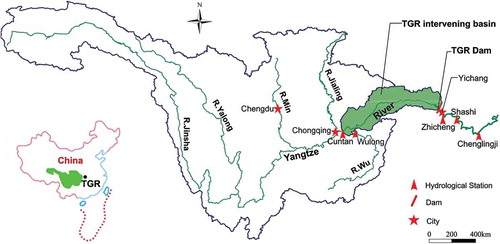
3.2 Deterministic inflow forecasts of the TGR

As shown in Figure 1, the inflow of the TGR has three components: the main upstream inflow (Cuntan station), the tributary inflow from the Wu River (Wulong station), and the lateral flow from the TGR intervening basin calculated by the Xinanjiang model (Zhao 1992, Cheng et al. 2006, Lin et al. 2014, Si et al. 2015). The multiple-input single-output linear systematic model was adopted to simulate the inflow of the TGR (Liang et al. 1992); for more details please refer to Li et al. (2010b) and Chen et al. (2015).

The whole data set ranged from 2003 to 2009, of which the period 2003–2007 was used for model calibration and 2008–2009 was used for validation. The simulation results for the NSE and RE in the calibration period are 97.72% and −1.04%, respectively, and in the verification period 95.84% and −0.21%, respectively. These results show that the deterministic forecast model is proven to be quite efficient in simulating the inflow series for the TGR.

4 Results and discussion

The forecasting in this study can be viewed as hindcasting essentially, in which the future rainfall is treated as perfect, and thus focuses on quantifying the hydrological uncertainty. The lead times are 24 h (n = 1), 48 h (n = 2) and 72 h (n = 3). The observed rainfalls are treated as the “perfect rainfall forecasts”, and are used to produce deterministic model inflows (s₁, s₂, s₃). They are attached to actual inflows (h₀, h₁, h₂, h₃) to obtain one joint realization of the model–actual inflow process. The dataset from 2003 to 2009 was used to calibrate and compare the meta-Gaussian HUP and copula-based HUP.

4.1 Determination of marginal distributions

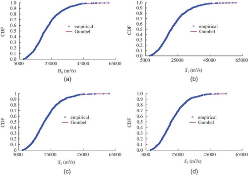
The sample series of H₀ was taken from 1 June to 27 September every year, S₁ from 2 June to 28 September, S₂ from 3 June to 29 September, and S₃ from 4 June to 30 September; thus, all these four variables have a data length of 833. The parameters of the six candidate distributions were estimated by the L-moment method and the results are listed in Table 3. The K-S test was used to verify the null hypothesis and the corresponding K-S statistic (D) values are reported in Table 4, which shows that the null hypothesis could not be rejected at the 5% significance level (critical value: 0.0471) for all six candidate distributions except the normal distribution. For the four hydrological variables, the Gumbel distribution provided the minimum D value and was chosen as the best fitting distribution. Figure 2 shows the empirical cdf values obtained from the Gringorten plotting-position formula (Zhang and Singh 2006) and theoretical cdf values calculated by the Gumbel distributions. It can be seen that the theoretical values fit the empirical values very well. For comparison purposes, the copula-based HUP used the same marginal distributions as the meta-Gaussian HUP in this paper.

Table 3. Parameter estimation results for four marginal distributions.

Variable	Normal		Gamma		Gumbel		Pearson type III			Log-normal		Log-Weibull
H0	22 354.30	8454.22	6.74	3318.06	6881.34	18 382.28	4.08	0.00023	4741.82	9.94	0.39	9.79	19.48	6109
S1	22 314.90	8393.89	6.81	3275.31	6832.24	18 371.22	3.92	0.00022	4639.73	9.94	0.39	9.79	19.52	6132
S2	22 240.16	8140.83	7.21	3084.93	6626.25	18 415.39	4.43	0.00024	3979.82	9.94	0.38	9.80	20.36	5991
S3	21 897.76	7763.05	7.70	2842.82	6318.76	18 250.47	5.95	0.00031	2670.46	9.93	0.37	9.78	20.88	5985

Table 4. Results of Kolmogorov-Smirnov test statistic D for four marginal distributions.

Variable	Normal	Gamma	Gumbel	Pearson type III	Log-normal	Log-Weibull
H0	0.0780	0.0306	0.0172	0.0219	0.0219	0.0244
S1	0.0780	0.0266	0.0183	0.0246	0.0246	0.0207
S2	0.0717	0.0467	0.0255	0.0264	0.0264	0.0263
S3	0.0720	0.0467	0.0178	0.0181	0.0181	0.0270

Figure 2. Empirical and theoretical values fitted by Gumbel distributions.

4.2 Calibration of copula-based HUP

The rank-based correlation (Kendall’s coefficient) matrix of variables H₀, H_n and S_n is shown in Table 5. It is demonstrated that the dependence among the three variable pairs (H₀, H_n), (H₀, S_n) and (H_n, S_n) is not the same. Furthermore, the highest correlation coefficient is exhibited in the variable pair (H_n, S_n). This result indicates that the asymmetric trivariate copula functions may be more appropriate than symmetric ones for use in the 3D joint distributions of H₀, H_n and S_n. When constructing the 3D joint distributions using the asymmetric copula functions, the structures (H_n, S_n)H₀ were applied. Specifically, the copula was first built for (H_n, S_n) and then for H₀ – .

Table 5. Ranked-based correlation matrix of the variables.

Lead times	Variables
24 h	H0, H1	0.823
	H0, S1	0.824
	H1, S1	0.929
48 h	H0, H2	0.694
	H0, S2	0.711
	H2, S2	0.883
72 h	H0, H3	0.600
	H0, S3	0.658
	H3, S3	0.828

The 3D joint distributions of H₀, H_n and S_n (n = 1, 2, 3) were constructed using the three candidate trivariate copula functions. Dependence parameters of the trivariate copula functions were estimated using the maximum pseudo-likelihood method and the results are listed in Table 6. It was found that the Frank copula performed best, with the smallest RMSE values for the three joint distributions. Empirical cdfs obtained from the Gringorten plotting-position formula and theoretical cdfs calculated from the Frank copula for the three joint distributions are plotted in Figure 3. An overall satisfactory agreement between the empirical and theoretical cdfs is shown. Hence, the asymmetric trivariate Frank copula functions have good performance in modelling the joint distributions of H₀, H_n and S_n.

Table 6. Estimated parameters of the three candidate copulas.

Variables	Gumbel-Hougaard		Frank		Clayton
	[θ1, θ2]	RMSE	[θ1, θ2]	RMSE	[θ1, θ2]	RMSE
H0, H1, S1	[9.08, 10.65]	0.0116	[25.44, 35.23]	0.0103	[15.16, 20.78]	0.0150
H0, H2, S2	[4.25, 7.58]	0.0141	[13.45, 20.38]	0.0112	[6.49, 14.33]	0.0186
H0, H3, S3	[2.98, 6.57]	0.0144	[9.58, 16.21]	0.0117	[4.58, 9.34]	0.0188

Figure 3. Plots of empirical and theoretical values estimated by Frank copulas for three joint cdfs. (Note: rank represents number of ordered pair, ranked in ascending order in terms of theoretical joint cdf, respectively.].

4.3 Comparison of the meta-Gaussian HUP and copula-based HUP

4.3.1 Posterior median forecasts

For 24-, 48- and 72-h lead times, the NSE and RE calculated by both the deterministic forecast model and posterior median forecasting associated with the meta-Gaussian HUP and copula-based HUP are listed in Table 7. It is shown that the results of both the meta-Gaussian HUP and the copula-based HUP are slightly better than those of the deterministic forecast model, and the copula-based HUP is comparable to the meta-Gaussian HUP. Compared with deterministic forecasts, the NSE and the RE of the copula-based HUP for 24-, 48- and 72-h lead time forecasts are improved by 1.24, 1.26 and 1.26% and reduced by 0.17, 0.57 and 1.72%, respectively. It is also noted that the accuracy of posterior median forecasts of the both HUPs decreases as the lead time increases.

Table 7. Comparison of performance evaluation criteria for deterministic forecasts.

Lead time	Deterministic model		Meta-Gaussian HUP		Copula-based HUP
	NSE (%)	RE (%)	NSE (%)	RE (%)	NSE (%)	RE (%)
24 h	97.55	–0.34	97.65	–0.31	98.79	–0.17
48 h	94.10	–0.85	94.54	–0.68	95.36	–0.28
72 h	88.52	–2.51	89.14	–1.14	89.78	–0.79

4.3.2 Probabilistic forecasts

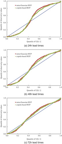
The predictive QQ plot, α-index, π-index and CRPS were adopted to evaluate the probabilistic forecasts. Figure 4 presents the predictive QQ plots with respect to the meta-Gaussian HUP and copula-based HUP for 24-, 48- and 72-h lead times. Using the guide presented in Thyer et al. (2009) to assess the results, it is clear that the overall performances of all predictive QQ plots are acceptable. Both the meta-Gaussian HUP and the copula-based HUP systematically under-predicted the inflows, since the observed p values at the theoretical median are a bit higher than the theoretical quantiles. In addition, the plots also show that the observed p values cluster around the tails (i.e. a high slope around theoretical quantile 0.4–0.6). This finding means that the predictive uncertainty is somewhat underestimated for both HUPs. The overall behaviours of the meta-Gaussian HUP and the copula-based HUP are found to be similar. The QQ plot for the copula-based HUP is slightly closer to the 1:1 line than for the meta-Gaussian HUP. That is to say, the copula-based HUP performs marginally better in terms of reliability. Nonetheless, these underestimations for both meta-Gaussian and copula-based HUPs are in zones where p values are relatively high, indicating that such differences may not be statistically significant.

Figure 4. Predictive QQ plots of meta-Gaussian HUP and copula-based HUP.

The results of α-index, π-index and CRPS are summarized in Table 8. For both the meta-Gaussian HUP and the copula-based HUP, it is clearly shown that the α-index value increases (higher reliability) when the lead time increases. However, it should be noted that this is at the expense of decreasing π-index values (lower resolution). Besides, the copula-based HUP has slightly larger α-index values, but smaller π-index values compared with the meta-Gaussian HUP. In terms of CRPS value, both HUPs outperform the deterministic forecasts, which demonstrates the effectiveness of probabilistic forecasts. Comparison results also indicate that the copula-based HUP is marginally better than the meta-Gaussian HUP. The CRPS value of the copula-based HUP for 24-, 48- and 72-h lead times is improved (decreased) by 16.6, 21.2 and 23.3%, respectively.

Table 8. Comparison of performance evaluation criteria for probabilistic forecasts.

Lead time	Deterministic model	Meta-Gaussian HUP			Copula-based HUP
	CRPS/MAE	α-index	π-index	CRPS	α-index	π-index	CRPS
24 h	688	0.8028	18.55	608	0.8507	16.39	574
48 h	1180	0.8555	12.45	975	0.8916	10.42	930
72 h	1763	0.8879	9.13	1420	0.9184	7.68	1353

Note: α-index and π-index are dimensionless; the unit of CRPS is m³/s.

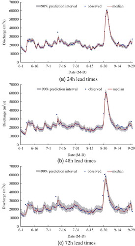
Although such marginally better performance does not result for each year, for illustrative purposes, the observed and median discharges, and 90% inflow prediction intervals estimated by the meta-Gaussian HUP and copula-based HUP in 2004 are presented in Figures 5 and 6, respectively. It can be seen that most observed inflows are contained within the 90% prediction intervals. This demonstrates that these 90% prediction intervals can effectively capture the forecast uncertainty and provide more information for decision making in flood control and reservoir operation. As lead time increases, the 90% prediction intervals become wider (i.e. greater uncertainty).

Figure 5. Meta-Gaussian HUP: 90% prediction intervals, median and observed discharges in 2004.

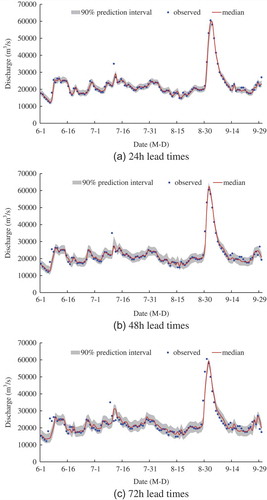
Figure 6. Copula-based HUP: 90% prediction intervals, median and observed discharges in 2004.

5 Summary and conclusions

Adequate assessment of uncertainty for flood forecasting is an important issue in hydrological research. Flood forecasting services are trending toward providing users with probabilistic forecasts, in place of traditional deterministic forecasts. This study has developed a copula-based HUP for probabilistic forecasting. The Three Gorges Reservoir (TGR) in China was selected as the case study and the results were compared with those of the widely used meta-Gaussian HUP. The main conclusions are summarized as follows:

1. The output of the HUP is a posterior distribution of the process, conditional upon the deterministic forecast. This posterior distribution provides a complete characterization of uncertainty, including quantiles with specified exceedence probabilities, prediction intervals with specified inclusion probabilities, and probabilities of exceedence for specified thresholds, which are needed by rational decision makers and information providers who want to extract forecast products for their customers.

2. Based on the copula function, the prior density and likelihood function of the HUP are explicitly expressed, and the corresponding posterior density and distribution can be obtained using the Monte Carlo sampling technique. This copula-based HUP can be implemented in the original space directly without a data transformation procedure into Gaussian space and allows for any form of marginal distribution of predictand and the deterministic forecast variable, and a nonlinear and heteroscedastic dependence structure.

3. Comparison results for the case study in China’s TGR demonstrate that the proposed copula-based HUP is comparable to the meta-Gaussian HUP in terms of the posterior median forecasts. It is also shown that probabilistic forecasts produced by the copula-based HUP have slightly higher reliability and lower resolution compared with the meta-Gaussian HUP. On the basis of the CRPS values, it is found that both HUPs are superior to deterministic forecasts, which highlights the effectiveness of probabilistic forecasts, and the copula-based HUP is marginally better than the meta-Gaussian HUP.

It is noted that the HUP discussed in this paper is for a univariate probabilistic forecast. This system independently provides a marginal probability distribution of observed discharge H_n (n = 1, 2, …, N) for each lead time; it does not consider and characterize the stochastic dependence among variables (H₁, H₂, …, H_N). A multivariate probabilistic forecast system (Krzysztofowicz and Maranzano 2004, Engeland and Steinsland 2014) would offer a joint probability distribution of (H₁, H₂, …, H_N) which would require a multivariate HUP and will be considered in further study.

Acknowledgements

The authors would like to thank the Hydrology Bureau of Changjiang Water Resources Commission and the China Three Gorges Corporation for providing the data used in this study.

Disclosure statement

No potential conflict of interest was reported by the authors.

Additional information

Funding

This study was financially supported by the National Natural Science Foundation of China [NSFC 51539009, 51525902] and the National Key Research and Development Plan of China [2016YFC0402206].

References

- Akhtar, M., Ahmad, N., and Booij, M.J., 2008. The impact of climate change on the water resources of Hindukush-Karakorum-Himalaya region under different glacier coverage scenarios. Journal of Hydrology, 355 (1), 148–163.
- Bárdossy, A. and Li, J., 2008. Geostatistical interpolation using copulas. Water Resources Research, 44, W07412. doi:10.1029/2007WR006115
- Berger, J.O., 1985. Statistical decision theory and Bayesian analysis. New York: Springer.
- Bergstrand, M., Asp, -S.-S., and Lindström, G., 2014. Nationwide hydrological statistics for Sweden with high resolution using the hydrological model S-HYPE. Hydrology Research, 45 (3), 349–356.
- Biondi, D. and De Luca, D.L., 2013. Performance assessment of a Bayesian Forecasting System (BFS) for real-time flood forecasting. Journal of Hydrology, 479 (1), 51–63.
- Biondi, D., Versace, P., and Sirangelo, B., 2010. Uncertainty assessment through a precipitation dependent hydrologic uncertainty processor: an application to a small catchment in southern Italy. Journal of Hydrology, 386 (1), 38–54.
- Bogner, K., Pappenberger, F., and Cloke, H.L., 2012. Technical Note: the normal quantile transformation and its application in a flood forecasting system. Hydrology and Earth System Sciences, 16 (4), 1085–1094.
- Calvo, B. and Savi, F., 2009. Real-time flood forecasting of the Tiber river in Rome. Natural Hazards, 50 (3), 461–477.
- Castellarin, A., Vogel, R.M., and Brath, A., 2004. A stochastic index flow model of flow duration curves. Water Resources Research, 40 (3). doi:10.1029/2003WR002524
- Chebana, F. and Quarda, T.B.M.J., 2011. Multivariate quantiles in hydrological frequency analysis. Environmetrics, 22 (1), 441–455.
- Chen, F.J., Jiao, M.Y., and Chen, J., 2013a. The meta-Gaussian Bayesian Processor of forecasts and associated preliminary experiments. Acta Meteorologica Sinica, 27, 199–210.
- Chen, L., et al., 2010. A new seasonal design flood method based on bivariate joint distribution of flood magnitude and date of occurrence. Hydrological Sciences Journal, 55 (8), 1264–1280.
- Chen, L., et al., 2013b. Measure of correlation between river flows using the copula-entropy method. Journal of Hydrologic Engineering, 18 (12), 1591–1606.
- Chen, L., et al., 2013c. Drought analysis using copulas. Journal of Hydrologic Engineering, 18 (7), 797–808.
- Chen, L., et al., 2014a. Copula entropy coupled with artificial neural network for rainfall-runoff simulation. Stochastic Environmental Research and Risk Assessment, 28 (7), 1755–1767.
- Chen, L., et al., 2014b. Determination of input for artificial neural networks for flood forecasting using the copula entropy method. Journal of Hydrologic Engineering, 19 (11), 04014021.
- Chen, L., et al., 2015. Real-time error correction method combined with combination flood forecasting technique for improving the accuracy of flood forecasting. Journal of Hydrology, 521, 157–169.
- Chen, S.T. and Yu, P.S., 2007. Real-time probabilistic forecasting of flood stages. Journal of Hydrology, 340 (1), 63–77.
- Chen, Y.-W., et al., 2014c. The development of a real-time flooding operation model in the Tseng-Wen Reservoir. Hydrology Research, 45 (3), 490–503.
- Cheng, C.T., et al., 2006. Using genetic algorithm and TOPSIS for Xinanjiang model calibration with a single procedure. Journal of Hydrology, 316 (1), 129–140.
- Coccia, G. and Todini, E., 2011. Recent developments in predictive uncertainty assessment based on the model conditional processor approach. Hydrology and Earth System Science, 15 (10), 3253–3274.
- Engeland, K., et al., 2010. Evaluation of statistical models for forecast errors from the HBV model. Journal of Hydrology, 384 (1), 142–155.
- Engeland, K. and Steinsland, I., 2014. Probabilistic post processing models for flow forecasts for a system of catchments and several lead times. Water Resources Research, 50 (1), 182–197.
- Evin, G., et al., 2014. Comparison of joint versus post processor approaches for hydrological uncertainty estimation accounting for error autocorrelation and heteroscedasticity. Water Resources Research, 50 (3), 2350–2375.
- Favre, A.C., et al., 2004. Multivariate hydrological frequency analysis using copulas. Water Resources Research, 40W01101. doi:10.1029/2003WR002456
- Freer, J., Beven, K., and Ambroise, B., 1996. Bayesian estimation of uncertainty in runoff prediction and the value of data: an application of the GLUE approach. Water Resources Research, 32 (7), 2161–2173.
- Genest, C. and Favre, A., 2007. Everything you always wanted to know about copula modeling but were afraid to ask. Journal of Hydrologic Engineering, 12 (4), 347–368.
- Gneiting, T., et al., 2005. Calibrated probabilistic forecasting using ensemble model output statistics and minimum CRPS estimation. Monthly Weather Review, 133 (5), 1098–1118.
- Gneiting, T., Balabdaoui, F., and Raftery, A.E., 2007. Probabilistic forecasts, calibration and sharpness. Journal of the Royal Statistical Society: Series B (Statistical Methodology), 69 (2), 243–268.
- Gottschalk, L., et al., 2013. Statistics of low flow: theoretical derivation of the distribution of minimum streamflow series. Journal of Hydrology, 481, 204–219.
- Guo, S.L., et al., 2004. A reservoir flood forecasting and control system for China. Hydrological Sciences Journal, 49 (6), 959–972.
- Hersbach, H., 2000. Decomposition of the continuous ranked probability score for ensemble prediction systems. Weather and Forecasting, 15 (5), 559–570.
- Hosking, J.R.M., 1990. L-moments: analysis and estimation of distributions using linear combinations of order statistics. Journal of the Royal Statistical Society, 52 (1), 105–124.
- Kasiviswanathan, K.S., et al., 2013. Constructing prediction interval for artificial neural network rainfall runoff models based on ensemble simulations. Journal of Hydrology, 499, 275–288.
- Koutsoyiannis, D. and Montanari, A., 2015. Negligent killing of scientific concepts: the stationarity case. Hydrological Sciences Journal, 60 (7–8), 1174–1183.
- Kroese, D.P., Taimre, T., and Botev, Z.I., 2013. Handbook of Monte Carlo Methods. New York: John Wiley.
- Krzysztofowicz, R., 1999. Bayesian theory of probabilistic forecasting via deterministic hydrologic model. Water Resources Research, 35 (9), 2739–2750.
- Krzysztofowicz, R. and Kelly, K.S., 2000. Hydrologic uncertainty processor for probabilistic river stage forecasting. Water Resources Research, 36 (11), 3265–3277.
- Krzysztofowicz, R. and Maranzano, C.J., 2004. Hydrologic uncertainty processor for probabilistic stage transition forecasting. Journal of Hydrology, 293 (1), 57–73.
- Laio, F. and Tamea, S., 2007. Verification tools for probabilistic forecasts of continuous hydrological variables. Hydrology and Earth System Sciences, 11 (4), 1267–1277.
- Li, H., Beldring, S., and Xu, C.-Y., 2014. Implementation and testing of routing algorithms in the distributed HBV model for mountainous catchments. Hydrology Research, 45 (3), 322–333.
- Li, L., et al., 2010a. Evaluation of the subjective factors of the GLUE method and comparison with the formal Bayesian method in uncertainty assessment of hydrological models. Journal of Hydrology, 390 (3), 210–221.
- Li, T.Y., et al., 2013. Bivariate flood frequency analysis with historical information based on copula. Journal of Hydrologic Engineering. doi:10.1061/(ASCE)HE.1943-5584.0000684
- Li, X., et al., 2010b. Dynamic control of flood limited water level for reservoir operation by considering inflow uncertainty. Journal of Hydrology, 391, 124–132.
- Liang, G.C., et al., 1992. River flow forecasting. Part 4. Applications of linear modeling techniques for flow routing on large basins. Journal of Hydrology, 133 (1), 99–140.
- Lin, K., et al., 2014. Xinanjiang model combined with Curve Number to simulate the effect of land use change on environmental flow. Journal of Hydrology, 519, 3142–3152.
- Liu, Z., et al., 2010. Impacts of climate change on hydrological processes in the headwater catchment of the Tarim River basin, China. Hydrological Processes, 24 (2), 196–208.
- Liu, Z., et al., 2016. Comparative study of three updating procedures for real-time flood forecasting. Water Resources Management, 30 (7), 2111–2126.
- Liu, Z., et al., 2017. The impact of Three Gorges Reservoir refill operation on water levels in Poyang Lake, China. Stochastic Environmental Research and Risk Assessment, 31 (4), 879–891.
- Liucci, L., Valigi, D., and Casadei, S., 2014. A new application of Flow Duration Curve (FDC) in designing run-of-river power plants. Water Resources Management, 28 (3), 881–895.
- Ma, H., et al., 2010. Impact of climate variability and human activity on streamflow decrease in the Miyun Reservoir catchment. Journal of Hydrology, 389 (3), 317–324.
- Ma, Z.K., et al., 2013. Bayesian statistic forecasting model for middle-term and long-term runoff of a hydropower station. Journal of Hydrologic Engineering, 18 (11), 1458–1463.
- Madadgar, S., Moradkhani, H., and Garen, D., 2014. Towards improved post-processing of hydrologic forecast ensembles. Hydrological Processes, 28 (1), 104–122.
- Montanari, A., 2007. What do we mean by ‘uncertainty’? The need for a consistent wording about uncertainty assessment in hydrology. Hydrological Processes, 21 (6), 841–845.
- Montanari, A. and Grossi, G., 2008. Estimating the uncertainty of hydrological forecasts: A statistical approach. Water Resources Research, 44, W00B08. doi:10.1029/2008WR006897
- Nash, J. and Sutcliffe, J.V., 1970. River flow forecasting through conceptual models part I—A discussion of principles. Journal of Hydrology, 10 (3), 282–290.
- Nelsen, R.B., 2006. An Introduction to copulas. Second. New York: Springer.
- Pappenberger, F., et al., 2015. How do I know if my forecasts are better? Using benchmarks in hydrological ensemble prediction. Journal of Hydrology, 522, 697–713.
- Pokhrel, P., Robertson, D.E., and Wang, Q.J., 2013. A Bayesian joint probability post-processor for reducing errors and quantifying uncertainty in monthly streamflow predictions. Hydrology and Earth System Science, 17 (2), 795–804.
- Rahman, M.M., et al., 2010. Design flow and stage computations in the Teesta River, Bangladesh, using frequency analysis and MIKE 11 modeling. Journal of Hydrologic Engineering, 16 (2), 176–186.
- Ramos, M.H., Van Andel, S.J., and Pappenberger, F., 2013. Do probabilistic forecasts lead to better decisions? Hydrology and Earth System Science, 17 (6), 2219–2232.
- Ravines, R.R., et al., 2008. A joint model for rainfall-runoff: the case of Rio Grande Basin. Journal of Hydrology, 353 (1), 189–200.
- Reggiani, P. and Weerts, A.H., 2008. A Bayesian approach to decision-making under uncertainty: an application to real-time forecasting in the river Rhine. Journal of Hydrology, 356 (1), 56–69.
- Renard, B., et al., 2010. Understanding predictive uncertainty in hydrologic modeling: the challenge of identifying input and structural errors. Water Resources Research, 46 (5). doi:10.1029/2009WR008328
- Robert, C. and Casella, G., 2013. Monte Carlo statistical methods. New York: Springer.
- Salvadori, G. and De Michele, C., 2007. On the use of copulas in hydrology: theory and practice. Journal of Hydrologic Engineering, 12 (4), 369–380.
- Shao, Q., et al., 2009. A new method for modelling flow duration curves and predicting streamflow regimes under altered land-use conditions. Hydrological Sciences Journal, 54 (3), 606–622.
- Si, W., Bao, W., and Gupta, H.V., 2015. Updating real-time flood forecasts via the dynamic system response curve method. Water Resources Research, 51 (7), 5128–5144.
- Sikorska, A.E., et al., 2012. Bayesian uncertainty assessment of flood predictions in ungauged urban basins for conceptual rainfall-runoff models. Hydrology and Earth System Science, 16 (4), 1221–1236.
- Smith, L.A., et al., 2015. Towards improving the framework for probabilistic forecast evaluation. Climatic Change, 132 (1), 31–45.
- Thyer, M., et al., 2009. Critical evaluation of parameter consistency and predictive uncertainty in hydrological modeling: A case study using Bayesian total error analysis. Water Resources Research, 45 (12). doi:10.1029/2008WR006825
- Tsai, C.N., Adrian, D.D., and Singh, V.P., 2001. Finite Fourier probability distribution and applications. Journal of Hydrologic Engineering, 6 (6), 460–471.
- Verkade, J.S. and Werner, M.G.F., 2011. Estimating the benefits of single value and probability forecasting for flood warning. Hydrology and Earth System Science, 15 (12), 3751–3765.
- Vogel, R.M. and Fennessey, N.M., 1994. Flow-duration curves. I: new interpretation and confidence intervals. Journal of Water Resources Planning and Management, 120 (4), 485–504.
- Vogel, R.M. and Fennessey, N.M., 1995. Flow-duration curves. II: A review of applications in water resources planning. Journal of the American Water Resources Association, 31 (6), 1029–1039.
- Weerts, A.H., Winsemius, H.C., and Verkade, J.S., 2011. Estimation of predictive hydrological uncertainty using quantile regression: examples from the national flood forecasting system (England and Wales). Hydrology and Earth System Science, 15 (1), 255–265.
- Wetterhall, F., et al., 2013. Forecasters priorities for improving probabilistic flood forecasts. Hydrology and Earth System Science Discuss, 10, 2215–2242. doi:10.5194/hessd-10-2215-2013
- Xiong, L., et al., 2015. Non-Stationary annual maximum flood frequency analysis using the norming constants method to consider non-Stationarity in the annual daily flow series. Water Resources Management, 29 (10), 3615–3633.
- Xiong, L.H., et al., 2009. Indices for assessing the prediction bounds of hydrological models and application by generalised likelihood uncertainty estimation. Hydrological Sciences Journal, 54 (5), 852–871.
- Xiong, L.H. and Guo, S.L., 1999. A two-parameter monthly water balance model and its application. Journal of Hydrology, 216 (1), 111–123.
- Xiong, L.H., Yu, K.X., and Gottschalk, L., 2014. Estimation of the distribution of annual runoff from climatic variables using copulas. Water Resources Research. doi:10.1029/2008WR006897
- Yokoo, Y. and Sivapalan, M., 2011. Towards reconstruction of the flow duration curve: development of a conceptual framework with a physical basis. Hydrology and Earth System Sciences, 15 (9), 2805–2819.
- Yu, K.X., Xiong, L.H., and Gottschalk, L., 2014. Derivation of low flow distribution functions using copulas. Journal of Hydrology, 508, 273–288.
- Zhang, J.H., et al., 2015. Determination of the distribution of flood forecasting error. Natural Hazards, 75 (2), 1389–1402.
- Zhang, L. and Singh, V.P., 2006. Bivariate flood frequency analysis using the copula method. Journal of Hydrologic Engineering, 11 (2), 150–164.
- Zhang, L. and Singh, V.P., 2007a. Bivariate rainfall frequency distributions using Archimedean copulas. Journal of Hydrology, 332 (1), 93–109.
- Zhang, L. and Singh, V.P., 2007b. Gumbel-Hougaard copula for trivariate rainfall frequency analysis. Journal of Hydrologic Engineering, 12 (4), 409–419.
- Zhang, L. and Singh, V.P., 2007c. Trivariate flood frequency analysis using the Gumbel-Hougaard copula. Journal of Hydrologic Engineering, 12 (4), 431–439.
- Zhang, Q., et al., 2011. Copula-based analysis of hydrological extremes and implications of hydrological behaviors in the Pearl River basin, China. Journal of Hydrologic Engineering, 16 (7), 598–607.
- Zhang, Q., et al., 2013. Copula-based spatio-temporal patterns of precipitation extremes in China. International Journal of Climatology, 33 (5), 1140–1152.
- Zhang, Q., Li, J., and Singh, V.P., 2012. Application of Archimedean copulas in the analysis of the precipitation extremes: effects of precipitation changes. Theoretical and Applied Climatology, 107 (1–2), 255–264.
- Zhao, R.J., 1992. The Xinanjiang model applied in China. Journal of Hydrology, 135 (1–4), 371–381.
- Zhao, T., et al., 2015. Quantifying predictive uncertainty of streamflow forecasts based on a Bayesian joint probability model. Journal of Hydrology, 528, 329–340.