Modelling long-term groundwater fluctuations by extreme learning machine using hydro-climatic data

ABSTRACT

The ability of the extreme learning machine (ELM) is investigated in modelling groundwater level (GWL) fluctuations using hydro-climatic data obtained for Hormozgan Province, southern Iran. Monthly precipitation, evaporation and previous GWL data were used as model inputs. Developed ELM models were compared with the artificial neural networks (ANN) and radial basis function (RBF) models. The models were also compared with the autoregressive moving average (ARMA), and evaluated using mean square errors, mean absolute error, Nash-Sutcliffe efficiency and determination coefficient statistics. All the data-driven models had better accuracy than the ARMA, and the ELM model’s performance was superior to that of the ANN and RBF models in modelling 1-, 2- and 3-month-ahead GWL. The RMSE accuracy of the ANN model was increased by 37, 34 and 52% using ELM for the 1-, 2- and 3-month-ahead forecasts, respectively. The accuracy of the ELM models was found to be less sensitive to increasing lead time.

KEYWORDS:

• groundwater level fluctuations
• long-term forecasting
• extreme learning machine (ELM)
• artificial neural networks (ANN)
• radial basis function (RBF)

Editor R. Woods Associate editor A. Jain

1 Introduction

Groundwater has vital importance for industry, agriculture and wildlife, especially, in arid and semi-arid environments. In such regions (arid and semi-arid), rainfall is highly variable and considerably lower than the evapotranspiration rate; therefore, groundwater can be the main component of the water resource (Jolly et al. 2008, Mirzavand and Ghazavi 2015). In Iran, groundwater is the main source of water supply for agricultural, industrial and domestic uses.

During the past decade, soft computing techniques have been successfully employed in different branches of water resources engineering (e.g. Daliakopoulos et al. 2005, Krishna et al. 2008, Banerjee et al. 2009, Ghose et al. 2010, Adamowski and Chan 2011, Garg 2014, Nikoo et al. 2016, Mirzavand et al. 2017, Valizadeh et al. 2017). Mohanty et al. (2010) applied an artificial neural network (ANN) model to forecast groundwater fluctuations in a river island of eastern India. They evaluated the performance of three different gradient-based training algorithms for the ANN. The results of this study showed the feasibility of employing training algorithms in modelling time series. Emamgholizadeh et al. (2014) applied an ANN model and an adaptive neuro-fuzzy inference system (ANFIS) to estimate groundwater fluctuations of Bastam Plain in Iran. As demonstrated in the study, the ANFIS offered the most promising results compared to the ANN model. Juan et al. (2015) developed ANN-based models for estimating groundwater fluctuations due to climate change in the Zuomaoxikong watershed of the Fenghuo Mountains, China. The obtained results showed the good accuracy and high validity of ANN models in predicting groundwater level (GWL) variation. Khalil et al. (2015) investigated the applicability of wavelet ensemble neural network (WENN), ANN and multiple linear regression (MLR) models for forecasting GWL in Manitou mine, Val-d’Or, in Quebec, Canada. They found that the reliability of WENN model was better than that of the ANN and MLR models for predicting GWL.

Kisi and Parmar (2016) investigated the ability of the least square support vector machine (LSSVM), multivariate adaptive regression splines (MARS) and M5 Model Tree (M5Tree) in forecasting pollution of river water. The study revealed that the LSSVM and MARS models could be used successfully to forecast monthly river water pollution. Barzegar et al. (2016) evaluated the ability of ANN, ANFIS, wavelet-ANN and wavelet-ANFIS models in modelling water salinity levels of northwest Iran’s Aji-Chay River. The wavelet-ANFIS models showed better performance than the other models in predicting water quality.

The extreme learning machine (ELM) model is a new learning algorithm for single hidden layer feedforward neural networks (SLNFNs) suggested by Huang et al. (2004). The ELM selects the input weights randomly and calculates the output weights analytically. The ELM has been employed in different fields of study (e.g. Deo and Şahin 2014, Abdullah et al. 2015, Deo et al. 2017, Sajjadi et al. 2016, Sokolov-Mladenović et al. 2016). This novel learning method has some priorities in comparison with conventional learning methods for neural networks, including: (1) the ELM is not only valid for sigmoid type of hidden neurons; indeed, its universal approximation capability has been proved for almost any nonlinear piecewise continuous hidden neurons (Huang, 2014); (2) the ELM is easy to use, fast, and provides good generalization performance; (3) the ELM is capable of determining all the network parameters such as learning rate, learning epochs and local minima analytically, which avoids human intervention; and (4) different nonlinear and kernel functions are employed in the ELM (Huang et al. 2004).

Shamshirband et al. (2015) investigated the ability of a kernel extreme learning machine (KELM) and support vector regression (SVR) in forecasting daily global solar radiation in Bandar Abass, Iran. The study indicated that the KELM model could be used successfully to forecast solar radiation. Mohammadi et al. (2015) employed three data-driven models – ELM, ANN and SVM – for forecasting daily dew point temperature in Bandar Abass and Tabass stations, Iran. Their results showed that the ELM models performed better than the ANN and SVM models. Deo and Şahin (2016) investigated the applicability of ELM and ANN models for prediction of monthly mean streamflow water levels in Queensland, Australia. The results revealed that the ELM performed better than the ANN model in forecasting streamflow water levels.

The aim of this study was to explore the use of the ELM method for monthly GWL forecasting and to compare it with two different neural networks and a stochastic method. The ELM models were developed and compared with ANN, RBF and ARMA models for 1-, 2- and 3-month-ahead forecasting of GWL in the Shamil-Ashekara Plain, Iran. The novelty of our study is to develop and apply an ELM model for simulation of monthly GWL fluctuation using climatic variables.

2 Study area

The study area selected for this research is the Shamil-Ashekara Plain, which is located in Hormozgan Province in the southern part of Iran (Fig. 1). It is located between 55º53′–56º19′E latitude and 28º4′–28º18′N longitude. The total area of the plain is 1106 km². The study area has an arid and sub-humid climate with an average annual rainfall of 370 mm, which occurs mostly in winter and autumn. The normal mean monthly minimum and maximum temperatures of the study area are 16.7 and 47ºC in January and August, respectively. In the study area, groundwater is the main source of irrigation. Because of the increasing demand on water supply, monitoring of the water table is needed by water managers to evaluate current and long-term groundwater conditions in the Shamil-Ashekara Plain.

3 Methods

3.1 Artificial neural networks

Artificial neural networks (ANNs), which are based on artificial intelligence (AI) methods, are parallel information processing structures inspired by the biological models of neurons. In this study, simulation of the water table levels in Shamil-Ashekara Plain was considered by using three different types of ANN: the multilayer perceptron (MLP) with the Levenberg-Marquardt training algorithm, the radial basis function (RBF), and the extreme learning machine (ELM).

It is worth noting that MLP and RBF neural networks are widely used neural network approaches and are known as the general forms of ANNs (Senthil Kumar et al. 2005; Zounemat-Kermani et al. 2013). In addition to applying MLP and RBF, the ELM, which is a novel and fast learning neural network, is also utilized and assessed. Therefore, the aim of this paper is the comparative evaluation of the performances of these types of ANNs for simulating the water table levels. These methods are described in the following subsections.

3.2 Multilayer perceptron neural networks (MLP)

Multilayer perceptrons are the best known and most used ANNs in the water engineering field and in hydrological modelling. These types of networks are structured with one input layer, one or more hidden layers, and one output layer. In each layer there are neurons. As for the input and output layer, the neurons are equivalent to the input and output variables. But the optimum number of neurons in the hidden layer(s) is not a priori specified and might be obtained from a simple trial-and-error procedure. Neurons in each layer are connected with neurons in the following layer by synaptic weights (Zounemat-Kermani 2012, Kisi et al. 2016). After summing up their inputs, neurons produce their output through activation functions. The relationship that describes the input/output relationship of a time series dataset for the MLP network is as follows:

(1)

where is the network output (i = 1, 2, …, number of targets); g is the transfer/activation function of the q neurons in the hidden layer; x_k stands for the input value (previous values of GWL, evapotranspiration and precipitation); p is the number of elements for the input vector, w_jk; and β_ij are the synaptic weights of neuron j connecting the input and output of the neuron j at the hidden layer. In general, MLPs use sigmoidal transfer functions for universal approximation (Fig. 2(a)).

Via the back-propagation process, the adjustable weights of connections are modified based on the residual between the computed values and the given target values at the output layer. It is obvious that at the first epoch the predicted output values are different from the target ones. In this study, the unknown parameters of the network (weights) are estimated by means of a quasi-Newton algorithm (the Levenberg-Marquardt algorithm). Hence, the feedforward process repeats the calculation process for modifying interconnected weights until an target total error (e.g. the mean square error, MSE) or number of prescribed iterations (epoch) is reached (Kisi 2006). More details on MLP neural networks and the Levenberg-Marquardt algorithm can be seen in Okkan (2011) and Zounemat-Kermani (2012).

3.3 Radial basis function neural network (RBF)

The RBF networks have been applied in many time series simulation problems as an alternative to the common MLP neural networks (Fernando and Jayawardena 1998, Yu and Yu 2012, Ahmed et al. 2015). Similarly to the MLP neural network, the RBF network has a three-layer architecture including one input, one hidden and one output layer (note that in the RBF network only one hidden layer is presumed). The neurons in the network within each layer are connected to the neurons of the previous layer. Unlike MLP networks, there are no synaptic weights between the input vector and the hidden layer. Hence, the first (input) layer passes inputs to the second (hidden) layer without changing their values. Each neuron in the hidden layer uses an RBF as the transfer function. The output of the RBF network can be described by the following equation (Yu and Yu 2012, Ahmed et al. 2015):

(2)

Similarly to the MLP formulation (Equation (1)), is the network output and β_ij are the synaptic weights of neuron j connecting the input and output of the neuron j. Other parameters were introduced in the previous section. In Equation (2), g_j is a radial symmetric transfer (activation) function (normally a Gaussian shape activation function) which can be represented as:

(3)

where μ_j and σ_j are, respectively, the centroid and the spread of the Gaussian function for neuron j. Adjusting the parameters in an RBF network is normally done in two phases. In the first phase, centroids and spreads of the Gaussian transfer functions are determined according to the training data. In the second phase a linear estimation of weighting vectors using ordinary least squares is considered. Several training algorithms can be used for calculating the adjustable parameters in RBF networks, including a derivative-based optimization algorithm (e.g. gradient descent algorithm) and meta-heuristic algorithms (e.g. genetic algorithm). In this study, the gradient descent algorithm is applied for the learning process of the RBF network. Figure 2(b) presents the general architecture of an RBF neural network.

Figure 1. Location of the study area.

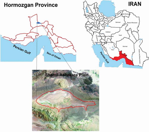
Figure 2. Network architecture of (a) three-layer MLP/ELM and (b) RBF neural networks.

3.4 Extreme learning machine neural network (ELM)

The ELM approach was proposed to overcome and mitigate the drawbacks of conventional training techniques (e.g. high computational cost) in MLP neural networks (Huang et al. 2006, Bueno-Crespo et al. 2013). In addition to its simplicity, applying this type of training algorithm makes the calculation faster and more accurate in comparison to the traditional training techniques of MLP networks, such as the gradient descent-based methods. The ELM algorithm randomly sets the network weights to the computational nodes in the hidden layer of an MLP-type neural network and only the output weights are adjusted during the training phase. In this regard, the standard ELM algorithm is based on an MLP consisting of q hidden neurons, whose input weights are randomly initialized, being able to learn p different k-dimensional input vectors producing zero error (see Equation (1)). Regarding the ELM algorithm, it can be shown that MLP can approximate p cases with zero error , with being the output of the network and the target vector (Huang et al. 2006).

As already mentioned, MLP-ELM input weights are fixed to random values; therefore, the network performs as a linear system. Due to this fact the output weights can be obtained using the H matrix (the pseudo-inverse hidden neurons output) for a given training set (HB = Z; where B is the weight vector connecting the hidden nodes and the output nodes matrix and Z is the training data target matrix). A detailed description of the ELM model is given in Huang et al. (2006) and Huang (2014).

4 Application and results

The accuracy of the ELM was examined in predicting 1-, 2- and 3-month-ahead groundwater levels and the results were compared with those of the ANN, RBF neural networks and ARMA. It should be noted that the ANN indicates the multilayer perceptron neural networks in this study. Root mean square error (RMSE), mean absolute error (MAE), Nash-Sutcliffe efficiency (NS) and determination coefficient (R²) were used to investigate the accuracy of each applied model. The evaluation criteria used in the current study can be characterized as:

(4)

(5)

(6)

where N, GWL_i,o and GWL_i,e are the data number, observed and estimated groundwater levels, respectively, and is the mean of the observed GWL.

The data used for model development are monthly precipitation, evaporation and previous GWL values. The target is the GWL at time t + 1, t + 2 and t + 3. The optimal input combinations were identified using auto-, partial auto- and cross-correlation statistics. Before applying the ELM, ANN and RBF models, the data were normalized in the range between 0 and 1. The input combinations determined according to the correlation analysis are: (i) GWL_t−1 and GWL_t−2; (ii) GWL_t−1, GWL_t−2 and P_t; (iii) GWL_t−1, GWL_t−2 and E_t; (iv) GWL_t−1, GWL_t−2, P_t and E_t, referred to as Input1, Input2, Input3 and Input4, respectively. Here, GWL_t, P_t and E_t are, respectively, the groundwater level, precipitation and evaporation at time t. For the ELM models, different activation functions (see Table 1) and hidden node numbers were tried. The optimal number of hidden nodes was found to be 50. For the ANN models, hidden node numbers were calculated as twice the input numbers, following the approach of Bhattacharyya and Pendharkar (1998). Different activation functions were tried for the ANN models, and the sigmoid and linear functions were found to be the best for the hidden and output nodes, respectively. Also, 1000 iterations were found to be sufficient for obtaining the optimal models by trial and error. For the RBF models, different numbers of hidden nodes (from 5 to 40 in increments of 5) were used, and 35 was found to be optimal; 1000 iterations were also employed, similarly to the ANN models.

Table 1. RMSE, R², NS and MAE accuracies of different ELM models in prediction of 1-month-ahead GWL. Bold indicates the best input combination.

Inputs	Activation function					Activation function
	Sigmoid	Sine	Hardlim	Triang. basis	Radial basis	Sigmoid	Sine	Hardlim	Triang. basis	Radial basis
	RMSE					R^2
Input1
Train	0.0063	0.0064	0.0334	0.0087	0.0060	0.9991	0.9991	0.9754	0.9983	0.9992
Test	0.0236	0.0485	0.0399	0.0161	0.0783	0.9876	0.9542	0.9645	0.9949	0.8922
Input2
Train	0.0066	0.0073	0.0383	0.0081	0.0075	0.9990	0.9988	0.9677	0.9986	0.9988
Test	0.0409	0.0183	0.0409	0.0181	0.0194	0.9622	0.9927	0.9620	0.9930	0.9923
Input3
Train	0.0068	0.0072	0.0502	0.0112	0.0069	0.9990	0.9989	0.9446	0.9973	0.9990
Test	0.0129	0.0103	0.0540	0.0203	0.0139	0.9967	0.9978	0.9349	0.9907	0.9958
Input4
Train	0.0064	0.0064	0.0492	0.0082	0.0073	0.9991	0.9991	0.9468	0.9985	0.9988
Test	0.0127	0.0152	0.0568	0.0202	0.0176	0.9968	0.9954	0.9311	0.9913	0.9937
	NS					MAE
Input1
Train	0.9991	0.9991	0.9748	0.9983	0.9992	0.0028	0.0028	0.0237	0.004	0.0025
Test	0.9872	0.9519	0.9599	0.9938	0.8879	0.0086	0.0135	0.0263	0.0057	0.0217
Input2
Train	0.9990	0.9988	0.9666	0.9986	0.9988	0.0031	0.0038	0.0295	0.0038	0.0038
Test	0.9598	0.9921	0.9597	0.9922	0.9912	0.0132	0.0066	0.0335	0.0073	0.0075
Input3
Train	0.9990	0.9989	0.9413	0.9972	0.999	0.0038	0.0036	0.0379	0.007	0.0038
Test	0.9960	0.9975	0.9267	0.9906	0.9955	0.0077	0.0057	0.0414	0.0109	0.0073
Input4
Train	0.9991	0.9991	0.9438	0.9985	0.9988	0.0035	0.0034	0.0396	0.005	0.0038
Test	0.9963	0.9945	0.9118	0.9906	0.9925	0.0065	0.0075	0.0465	0.0101	0.0076

Table 1 illustrates the training and testing accuracies of the ELM models with respect to different activation functions in predicting 1-month-ahead GWLs. The ELM model utilizing the Input3 combination (GWL_t−1, GWL_t−2 and E_t) with sine activation function has the best accuracy (RMSE = 0.0103, R² = 0.9978, NS = 0.9975 and MAE = 0.0057) in the test period. The performance of each ELM model for forecasting 2-month-ahead GWLs is reported in Table 2. Here also the ELM model provides the best accuracy (RMSE = 0.0109, R² = 0.9975, NS = 0.9971 and MAE = 0.0060) with the Input3 combination and sine activation function in the test period. Table 3 gives the performance of different ELM models in forecasting 3-month-ahead GWLs. Similarly to the 1- and 2-month-ahead GWL forecasts, here also the best performance (RMSE = 0.0121, R² = 0.9969, NS = 0.9964 and MAE = 0.0060) was obtained from the Input3 combination and sine activation function in the test period. Comparison of accuracy ranges obviously indicates that increasing lead time decreases model accuracies, but not highly.

Table 2. RMSE, R², NS and MAE accuracies of different ELM models in prediction of 2-month-ahead GWL. Bold indicates the best input combination.

Inputs	Activation function					Activation function
	Sigmoid	Sine	Hardlim	Triang. basis	Radial basis	Sigmoid	Sine	Hardlim	Triang. basis	Radial basis
	RMSE					R^2
Input1
Train	0.0063	0.0063	0.0444	0.0075	0.0060	0.9991	0.9991	0.9569	0.9988	0.9992
Test	0.0425	0.0544	0.0431	0.0228	0.0823	0.9581	0.9313	0.9570	0.9889	0.8823
Input2
Train	0.0067	0.0071	0.0437	0.0086	0.0081	0.9990	0.9989	0.9582	0.9984	0.9986
Test	0.0430	0.0190	0.0474	0.0182	0.0251	0.9573	0.9919	0.9551	0.9926	0.9856
Input3
Train	0.0070	0.0072	0.0588	0.0103	0.0066	0.9989	0.9989	0.9245	0.9977	0.9990
Test	0.0117	0.0109	0.0621	0.0212	0.0155	0.9969	0.9975	0.9136	0.9902	0.9953
Input4
Train	0.0069	0.0075	0.0547	0.0116	0.0078	0.9990	0.9988	0.9347	0.9971	0.9987
Test	0.0127	0.0200	0.0682	0.0240	0.0193	0.9969	0.9907	0.8916	0.9868	0.9924
	NS					MAE
Input1
Train	0.9991	0.9991	0.9549	0.9988	0.9992	0.0026	0.0027	0.0323	0.0029	0.0024
Test	0.9542	0.9247	0.952	0.9883	0.8768	0.0131	0.0149	0.0319	0.0088	0.0223
Input2
Train	0.9990	0.9989	0.9564	0.9984	0.9986	0.0031	0.0035	0.0343	0.0047	0.0041
Test	0.9564	0.9913	0.934	0.9921	0.9853	0.0135	0.0068	0.0355	0.0079	0.01
Input3
Train	0.9989	0.9989	0.9183	0.9977	0.999	0.0037	0.0038	0.0451	0.0067	0.0035
Test	0.9968	0.9971	0.887	0.989	0.994	0.0066	0.0060	0.0476	0.0101	0.0078
Input4
Train	0.9990	0.9988	0.9301	0.9971	0.9987	0.0039	0.0042	0.0435	0.0073	0.0045
Test	0.9960	0.9903	0.8752	0.9859	0.991	0.0069	0.0088	0.0594	0.0128	0.0088

Table 3. RMSE and R² accuracies of different ELM models in prediction of 3-month-ahead GWL. Bold indicates the best input combination.

Inputs	Activation function					Activation function
	Sigmoid	Sine	Hardlim	Triang. basis	Radial basis	Sigmoid	Sine	Hardlim	Triang. basis	Radial basis
	RMSE					R^2
Input1
Train	0.0063	0.0063	0.0611	0.0063	0.0060	0.9991	0.9991	0.9183	0.9991	0.9992
Test	0.0647	0.0887	0.0487	0.0373	0.1541	0.9228	0.8719	0.9445	0.9708	0.7201
Input2
Train	0.0065	0.0068	0.0534	0.0078	0.0074	0.9991	0.9990	0.9378	0.9987	0.9988
Test	0.0448	0.0308	0.0593	0.0239	0.0306	0.9536	0.9778	0.9179	0.9872	0.9782
Input3
Train	0.0078	0.0082	0.0743	0.0085	0.0085	0.9987	0.9985	0.8793	0.9984	0.9984
Test	0.0146	0.0121	0.0826	0.0221	0.0214	0.9957	0.9969	0.8479	0.9894	0.9899
Input4
Train	0.0087	0.0083	0.0637	0.0120	0.0106	0.9984	0.9985	0.9113	0.9968	0.9976
Test	0.0158	0.0158	0.0716	0.0518	0.0246	0.9950	0.9947	0.8805	0.9471	0.9875
	NS					MAE
Input1
Train	0.9991	0.9991	0.9111	0.9991	0.9992	0.0027	0.0026	0.0430	0.0027	0.0024
Test	0.9183	0.8632	0.9397	0.9695	0.7009	0.0168	0.0203	0.0355	0.0117	0.0332
Input2
Train	0.9991	0.9990	0.9337	0.9987	0.9988	0.0031	0.0032	0.0420	0.0043	0.0038
Test	0.9517	0.9777	0.9133	0.9857	0.9781	0.0140	0.0097	0.0481	0.0099	0.0105
Input3
Train	0.9987	0.9985	0.8627	0.9984	0.9984	0.0038	0.0042	0.0569	0.0053	0.0046
Test	0.9947	0.9964	0.7713	0.9878	0.9889	0.0066	0.0060	0.0687	0.0102	0.0081
Input4
Train	0.9983	0.9985	0.9027	0.9968	0.9976	0.0051	0.0041	0.0505	0.0082	0.0065
Test	0.9938	0.9940	0.8673	0.9437	0.9860	0.0077	0.0058	0.0585	0.0185	0.0111

The accuracy of the ANN models in forecasting 1-, 2- and 3-month-ahead GWLs is reported in Table 4 with respect to RMSE, R², NS and MAE. In 1- and 2-month-ahead forecasts, the best results were obtained from the ANN with eight hidden nodes for the Input4 combination (GWL_t−1, GWL_t−2, P_t and E_t). For the 3-month lag, however, Input3 provided slightly better RMSE (0.0250) and NS (0.9855) than Input4 (0.0254 and 0.9852, respectively). Table 5 gives the performance of the RBF model in forecasting 1-, 2- and 3-month-ahead GWLs. For the RBF method, the Input4 combination provides the best accuracy in all three forecasts.

Table 4. RMSE, R², NS and MAE accuracies of different ANN models in prediction of GWL. Bold indicates the best model.

Model	Structure	Training				Test
		RMSE	R^2	NS	MAE	RMSE	R^2	NS	MAE
1-month-ahead
Input1	1-4-1	0.0076	0.9987	0.9987	0.0035	0.0189	0.9921	0.9914	0.0064
Input2	2-6-1	0.0071	0.9989	0.9989	0.0034	0.0186	0.9925	0.9916	0.0060
Input3	3-6-1	0.0071	0.9989	0.9989	0.0034	0.0194	0.9915	0.9909	0.0072
Input4	4-8-1	0.0054	0.9994	0.9994	0.0031	0.0163	0.9942	0.9936	0.0064
2-month-ahead
Input1	1-4-1	0.0070	0.9989	0.9989	0.0026	0.0238	0.9881	0.9859	0.0087
Input2	2-6-1	0.0070	0.9989	0.9989	0.0029	0.0188	0.9919	0.9910	0.0063
Input3	3-6-1	0.0062	0.9992	0.9992	0.0034	0.0233	0.9874	0.9870	0.0113
Input4	4-8-1	0.0064	0.9991	0.9991	0.0033	0.0166	0.9939	0.9934	0.0085
3-month-ahead
Input1	1-4-1	0.0063	0.9991	0.9991	0.0027	0.0595	0.9336	0.9298	0.0159
Input2	2-6-1	0.0066	0.9991	0.9991	0.0032	0.0514	0.9420	0.9417	0.0152
Input3	3-6-1	0.0063	0.9991	0.9991	0.0033	0.0250	0.9859	0.9855	0.0108
Input4	4-8-1	0.0065	0.9991	0.9991	0.0035	0.0254	0.9863	0.9852	0.0099

Table 5. RMSE, R², NS and MAE accuracies of different RBF models in prediction of GWL. Bold indicates the best model.

Models	Structure	Training				Test
		RMSE	R^2	NS	MAE	RMSE	R^2	NS	MAE
1-month-ahead
Input1	1-35-1	0.0069	0.9989	0.9989	0.0034	0.0188	0.9922	0.9913	0.0066
Input2	2-35-1	0.0071	0.9989	0.9989	0.0035	0.0252	0.9851	0.9844	0.0099
Input3	3-35-1	0.0079	0.9986	0.9986	0.0041	0.0177	0.9933	0.9923	0.0086
Input4	4-35-1	0.0081	0.9985	0.9985	0.0043	0.0159	0.9948	0.9937	0.0070
2-month-ahead
Input1	1-35-1	0.0069	0.9990	0.999	0.0034	0.0192	0.9919	0.9911	0.0073
Input2	2-35-1	0.0074	0.9988	0.9988	0.0039	0.0273	0.9846	0.9830	0.0105
Input3	3-35-1	0.0083	0.9985	0.9985	0.0039	0.0210	0.9904	0.9891	0.0077
Input4	4-35-1	0.0079	0.9986	0.9986	0.0041	0.0169	0.9942	0.9929	0.0072
3-month-ahead
Input1	1-35-1	0.0069	0.9990	0.999	0.0034	0.0192	0.9919	0.9911	0.0073
Input2	2-35-1	0.0075	0.9988	0.9988	0.0039	0.0305	0.9808	0.9792	0.0117
Input3	3-35-1	0.0083	0.9985	0.9985	0.0039	0.0210	0.9904	0.9891	0.0078
Input4	4-35-1	0.0080	0.9986	0.9986	0.0041	0.0188	0.9926	0.9912	0.0076

The accuracy of the optimal ELM, ANN, RBF and ARMA models is compared in Table 6. From Table 6, it is clearly seen that all the data-driven models have better efficiency than the ARMA models, and the ELM model performance is superior to that of the ANN and RBF models in 1-, 2- and 3-month-ahead GWL forecasting. While there is a slight difference between ANN and RBF in 1- and 2-month-ahead forecasts, the latter performs better than the first with a lower RMSE (0.0188) and MAE (0.0076) and higher R² (0.9926) and NS (0.9912) in forecasting 3-month-ahead GWLs. The best ELM models increase the RMSE accuracy of the ANN model by 37, 34 and 52% for the 1-, 2- and 3-month-ahead forecasts, respectively.

Table 6. Comparison of ELM, ANN and RBF models in forecasting monthly GWLs. Bold indicates the best model.

Models	Training				Test
	RMSE	R^2	NS	MAE	RMSE	R^2	NS	MAE
1-month-ahead
ELM	0.0072	0.9989	0.9989	0.0036	0.0103	0.9978	0.9975	0.0057
ANN	0.0054	0.9994	0.9994	0.0031	0.0163	0.9942	0.9936	0.0064
RBF	0.0081	0.9985	0.9985	0.0043	0.0159	0.9948	0.9937	0.0070
ARMA(2,1)	0.0859	0.8389	0.8079	0.0711	0.0946	0.7976	0.7902	0.0797
2-month-ahead
ELM	0.0072	0.9989	0.9989	0.0038	0.0109	0.9975	0.9971	0.0060
ANN	0.0064	0.9991	0.9991	0.0033	0.0166	0.9939	0.9934	0.0085
RBF	0.0079	0.9986	0.9986	0.0041	0.0169	0.9942	0.9929	0.0072
ARMA(2,1)	0.0887	0.8280	0.8280	0.0748	0.0947	0.7913	0.7898	0.0839
3-month-ahead
ELM	0.0082	0.9985	0.9985	0.0042	0.0121	0.9969	0.9964	0.0060
ANN	0.0063	0.9991	0.9991	0.0033	0.0250	0.9859	0.9855	0.0108
RBF	0.0080	0.9986	0.9986	0.0041	0.0188	0.9926	0.9912	0.0076
ARMA(2,1)	0.0953	0.8014	0.8014	0.0803	0.1050	0.7466	0.6088	0.0897

The observed and forecast 1-month-ahead GWLs by three different methods are shown in Figure 3 in the form of a time variation graph. The significant deviations are illustrated by circles in this figure. It is clear that, although the estimates of the all three methods closely follow the corresponding observed values, some considerable deviations are seen for the ANN and RBF models. The scatter plots of the model predictions for the 2-month interval in the test period are compared in Figure 4. It is clear from the fit line equations (assume the equation to be y = c₁x + c₂) that the c₁ and c₂ coefficients of the ELM model are closer to 1 and 0, with a higher R² value than those of the ANN and RBF models. Graphical comparison of three methods in forecasting 2- and 3-month-ahead GWLs is made in Figures 5–8 for the test period. The superior accuracy of ELM models over the ANN and RBF can be clearly seen from these figures for both intervals. The difference between the ELM and other methods increases by increasing time interval from 1 month to 3 months.

Overall, the ELM gives better accuracy than the ANN and RBF methods in forecasting groundwater fluctuations for three different intervals (1-, 2- and 3-month intervals). The advantages of the ELM over ANN and RBF models are that the ELM not only approximates the complex phenomenon, but it also does not need iteration during the training period. The ELM model, which has only a single hidden layer, is faster than the other two methods (Ding et al. 2015). The ELM can use various hidden activation functions as long as they are nonlinear piecewise continuous. This type of activation function does not need to be algebraic sum based. ELM theories do not need to consider the correct activation function formula of biological neurons, which, in fact, humans might not know the exact activation function of live brain neurons (Huang 2014). Therefore, the ELM method may be a good candidate for hydrological modelling.

Figure 3. Time variation graphs of the observed and forecast 1-month-ahead GWLs by ELM, ANN and RBF models in the test period. Circles indicate significant deviations.

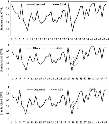
Figure 4. Scatter-plot graphs of the observed and forecast 1-month-ahead GWLs by ELM, ANN and RBF models in the test period.

Figure 5. Time variation graphs of the observed and forecast 2-month-ahead GWLs by ELM, ANN and RBF models in the test period. Circles indicate significant deviations.

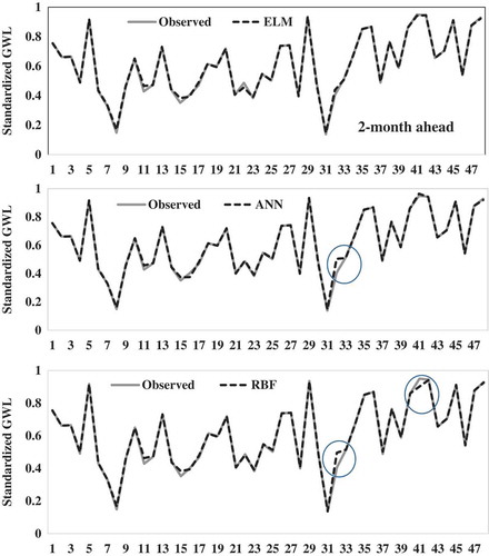
Figure 6. Scatter-plot graphs of the observed and forecast 2-month-ahead GWLs by ELM, ANN and RBF models in the test period.

Figure 7. Time variation graphs of the observed and forecast 3-month-ahead GWLs by ELM, ANN and RBF models in the test period. Circles indicate significant deviations.

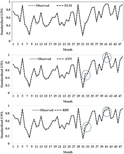
Figure 8. Scatter-plot graphs of the observed and forecast 3-month-ahead GWLs by ELM, ANN and RBF models in the test period.

5 Conclusions

In the current study, long-term groundwater level (GWL) fluctuations were modelled using the extreme learning machine (ELM) model. Precipitation, evaporation and previous GWL data obtained from Hormozgan province, Iran, were used as inputs to the models to forecast 1-, 2- and 3-month-ahead GWL fluctuations. The results of the optimal ELM models were compared with the conventional artificial neural networks (ANNs), radial basis function (RBF) and stochastic ARMA models with respect to mean square error, determination coefficient, time variation and scatter-plot graphs. Comparison revealed that the ARMA model provided the worst accuracy and the ELM method performance was superior to that of the other two data-driven methods in modelling 1-, 2- and 3-month-ahead GWLs. The radial basis function performance was superior to that of the ANNs in forecasting 3-month-ahead GWLs, while there is a slight difference between the two methods in 1- and 2-month-ahead forecasts. The ELM method may be used as a module in hydrological applications.

Disclosure statement

No potential conflict of interest was reported by the authors.

References

- Abdullah, S.S., et al., 2015. Extreme learning machines: a new approach for prediction of reference evapotranspiration. Journal of Hydrology, 527, 184–195. doi:10.1016/j.jhydrol.2015.04.073
- Adamowski, J. and Chan, H.F., 2011. A wavelet neural network conjunction model for groundwater level forecasting. Journal of Hydrology, 407 (1), 28–40. doi:10.1016/j.jhydrol.2011.06.013
- Ahmed, K., Shahid, S., and bin Harun, S., 2015. Statistical downscaling of rainfall in an arid coastal region: a radial basis function neural network approach. Applied Mechanics and materials. 735, 190–194.
- Banerjee, P., Prasad, R., and Singh, V., 2009. Forecasting of groundwater level in hard rock region using artificial neural network. Environmental Geology, 58 (6), 1239–1246. doi:10.1007/s00254-008-1619-z
- Barzegar, R., Adamowski, J., and Asghari Moghaddam, A., 2016. Application of wavelet-artificial intelligence hybrid models for water quality prediction: a case study in Aji-Chay River, Iran. Stochastic Environmental Research and Risk Assessment, 30 (7), 1797–1819.
- Bhattacharyya, S. and Pendharkar, P.C., 1998. Inductive, evolutionary, and neural computing techniques for discrimination: a comparative study. Decision Sciences, 29 (4), 871–899. doi:10.1111/deci.1998.29.issue-4
- Bueno-Crespo, A., García-Laencina, P.J., and Sancho-Gómez, J.L., 2013. Neural architecture design based on extreme learning machine. Neural Networks, 48, 19–24. doi:10.1016/j.neunet.2013.06.010
- Daliakopoulos, I.N., Coulibaly, P., and Tsanis, I., 2005. Groundwater level forecasting using artificial neural networks. Journal of Hydrology, 309 (1), 229–240. doi:10.1016/j.jhydrol.2004.12.001
- Deo, R.C., et al., 2017. Forecasting effective drought index using a wavelet extreme learning machine (W-ELM) model. Stochastic Environmental Research and Risk Assessment, 31 (5), 1211–1240.
- Deo, R.C. and Şahin, M., 2014. Application of the extreme learning machine algorithm for the prediction of monthly effective drought index in eastern Australia. Atmospheric Research, 153, 512–525. doi:10.1016/j.atmosres.2014.10.016
- Deo, R.C. and Şahin, M., 2016. An extreme learning machine model for the simulation of monthly mean streamflow water level in eastern Queensland. Environmental Monitoring and Assessment, 188 (2), 1–24.
- Ding, S., et al., 2015. Deep extreme learning machine and its application in EEG classification. Mathematical Problems in Engineering, 2015, Article ID 129021, 1–11. doi:10.1155/2015/129021
- Emamgholizadeh, S., Moslemi, K., and Karami, G., 2014. Prediction the groundwater level of bastam plain (Iran) by artificial neural network (ANN) and adaptive neuro-fuzzy inference system (ANFIS). Water Resources Management, 28 (15), 5433–5446. doi:10.1007/s11269-014-0810-0
- Fernando, D.A.K. and Jayawardena, A.W., 1998. Runoff forecasting using RBF networks with OLS algorithm. Journal of Hydrologic Engineering, 3 (3), 203–209. doi:10.1061/(ASCE)1084-0699(1998)3:3(203)
- Garg, V., 2014. Modeling catchment sediment yield: a genetic programming approach. Natural Hazards, 70, 39–50. doi:10.1007/s11069-011-0014-3
- Ghose, D.K., Panda, S.S., and Swain, P., 2010. Prediction of water table depth in western region, Orissa using BPNN and RBFN neural networks. Journal of Hydrology, 394 (3), 296–304. doi:10.1016/j.jhydrol.2010.09.003
- Huang, G.B., 2014. An insight into extreme learning machines: random neurons, random features and kernels. Cognitive Computation, 6 (3), 376–390. doi:10.1007/s12559-014-9255-2
- Huang, G.B., Zhu, Q.Y., and Siew, C.K., 2004. Extreme learning machine: a new learning scheme of feedforward neural networks. Neural Networks, 2004. Proceedings. 2004 IEEE International Joint Conference, 25–29 July. Budapest: IEEE.
- Huang, G.B., Zhu, Q.Y., and Siew, C.K., 2006. Extreme learning machine: theory and applications. Neurocomputing, 70 (1), 489–501. doi:10.1016/j.neucom.2005.12.126
- Jolly, I.D., McEwan, K.L., and Holland, K.L., 2008. A review of groundwater–surface water interactions in arid/semi-arid wetlands and the consequences of salinity for wetland ecology. Ecohydrology, 1 (1), 43–58. doi:10.1002/eco.6
- Juan, C., Wang, G., and Tianxu, M., 2015. Simulation and prediction of suprapermafrost groundwater level variation in response to climate change using a neural network model. Journal of Hydrology, 529, 1211–1220. doi:10.1016/j.jhydrol.2015.09.038
- Khalil, B., et al., 2015. Short-term forecasting of groundwater levels under conditions of mine-tailings recharge using wavelet ensemble neural network models. Hydrogeology Journal, 23 (1), 121–141. doi:10.1007/s10040-014-1204-3
- Kisi, O., 2006. Evapotranspiration estimation using feed-forward neural networks. Hydrology Research, 37 (3), 247–260. doi:10.2166/nh.2006.010
- Kisi, O., et al., 2016. Daily pan evaporation modeling using chi-squared automatic interaction detector, neural networks, classification and regression tree. Computers and Electronics in Agriculture, 122, 112–117. doi:10.1016/j.compag.2016.01.026
- Kisi, O. and Parmar, K.S., 2016. Application of least square support vector machine and multivariate adaptive regression spline models in long term prediction of river water pollution. Journal of Hydrology, 534, 104–112. doi:10.1016/j.jhydrol.2015.12.014
- Krishna, B., Satyaji Rao, Y., and Vijaya, T., 2008. Modelling groundwater levels in an urban coastal aquifer using artificial neural networks. Hydrological Processes, 22 (8), 1180–1188. doi:10.1002/(ISSN)1099-1085
- Mirzavand, M., et al., 2017. Evaluating groundwater level fluctuation by support vector regression and neuro-fuzzy methods: a comparative study. Natural Hazards. doi:10.1007/s11069-015-1602-4
- Mirzavand, M. and Ghazavi, R., 2015. A stochastic modelling technique for groundwater level forecasting in an arid environment using time series methods. Water Resour Manage, 29, 1315–1328. doi:10.1007/s11269-014-0875-9
- Mohammadi, K., et al., 2015. Extreme learning machine based prediction of daily dew point temperature. Computers and Electronics in Agriculture, 117, 214–225. doi:10.1016/j.compag.2015.08.008
- Mohanty, S., et al., 2010. Artificial neural network modeling for groundwater level forecasting in a river island of eastern India. Water Resources Management, 24 (9), 1845–1865. doi:10.1007/s11269-009-9527-x
- Nikoo, M., et al., 2016. Flood-routing modeling with neural network optimized by social-based algorithm. Natural Hazards, 82, 1–24. doi:10.1007/s11069-016-2176-5
- Okkan, U., 2011. Application of Levenberg-Marquardt optimization algorithm based multilayer neural networks for hydrological time series modeling. An International Journal of Optimization and Control: Theories & Applications (IJOCTA), 1 (1), 53–63.
- Sajjadi, S., et al., 2016. Extreme learning machine for prediction of heat load in district heating systems. Energy and Buildings, 122, 222–227. doi:10.1016/j.enbuild.2016.04.021
- Senthil Kumar, A.R., et al., 2005. Rainfall‐runoff modelling using artificial neural networks: comparison of network types. Hydrological Processes, 19 (6), 1277–1291. doi:10.1002/(ISSN)1099-1085
- Shamshirband, S., et al., 2015. Daily global solar radiation prediction from air temperatures using kernel extreme learning machine: A case study for city of Bandar Abass, Iran. Journal of Atmospheric and Solar-Terrestrial Physics, 134, 109–117. doi:10.1016/j.jastp.2015.09.014
- Sokolov-Mladenović, S., et al., 2016. Economic growth forecasting by artificial neural network with extreme learning machine based on trade, import and export parameters. Computers in Human Behavior, 65, 43–45. doi:10.1016/j.chb.2016.08.014
- Valizadeh, N., et al., 2017. Artificial intelligence and geo-statistical models for stream-flow forecasting in ungauged stations: state of the art. Natural Hazards, 86, 1377–1392. doi:10.1007/s11069-017-2740-7
- Yu, J.W. and Yu, J., 2012. Rainfall time series forecasting based on modular RBF neural network model coupled with SSA and PLS. Journal of Theoretical and Applied Computer Science, 6 (2), 3–12.
- Zounemat-Kermani, M., 2012. Hourly predictive Levenberg–marquardt ANN and multi linear regression models for predicting of dew point temperature. Meteorology and Atmospheric Physics, 117 (3–4), 181–192. doi:10.1007/s00703-012-0192-x
- Zounemat-Kermani, M., Kisi, O., and Rajaee, T., 2013. Performance of radial basis and LM-feed forward artificial neural networks for predicting daily watershed runoff. Applied Soft Computing, 13 (12), 4633–4644. doi:10.1016/j.asoc.2013.07.007