Raingauge network optimization in a tropical urban area by coupling cross-validation with the geostatistical technique

ABSTRACT

An adequate and reliable raingauge network is essential for observing rainfall data in hydrology and water resource applications. A raingauge network developed for a catchment area is commonly extended periodically to increase data accuracy. Due to financial constraints, the network is reviewed for the optimal number of stations. A new optimization approach is developed in this study by coupling a cross-validation technique with a geostatistical method for raingauge network optimization to prioritize raingauge stations. The spatial interpolation error of the spatial rainfall distribution, measured as the root mean square error (E_rms) optimization criterion is applied to a raingauge network in a tropical urban area. The results indicate that this method can successfully optimize the number of rainfall stations in an existing raingauge network, as the stations are prioritized based on their importance in the network.

KEYWORDS:

• raingauge network
• cross-validation
• geostatistical analysis
• optimization
• root mean square error

Editor D. Koutsoyiannis Associate editor E. Volpi

Introduction

A raingauge network is a hydrometric network meant to collect rainfall data and facilitate hydrology applications, such as hydrological modelling (Xu et al. 2015), flood forecasting (Kar et al. 2015), and flash flood prediction (Volkmann et al. 2010) as well as water resource analysis. Rainfall data from a raingauge network are used to compute spatial rainfall information in terms of areal average, point-based and spatial variability. Accurate rainfall data are very important for hydrology and water resource-related projects at the planning, design and operational levels (Adhikary et al. 2015).

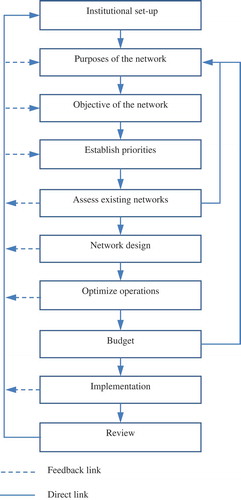
The rainfall data from raingauge networks involve point-based rainfall that is used to compute areal average rainfall for spatial rainfall mapping for instance. The map is produced through an interpolation process using point rainfall values. Accurate rainfall maps are extremely important for any hydrology application. The spatial rainfall interpolation error, measured as root mean square error (E_rms) is commonly used as an accuracy indicator. For example, Ali and Othman (2017) employed E_rms as an accuracy indicator to study the best variogram to produce an accurate spatial rainfall map. The spatial interpolation error should be as small as possible, which is achievable with an appropriate number of point rainfall values. The development of a raingauge network is an evolutionary process, beginning with the initial development of a basic network, followed by periodic reviews for upgrading to achieve an optimum network (Vivekanandan and Jagtap 2013). River basin managers around the world adopt this process in raingauge network design and optimization. A raingauge network is reviewed to optimize the appropriate number of point rainfall stations, as studied by Bastin et al. (1984) and Pardo-Igúzquiza (1998). The review process may be based on the procedure suggested by the World Meteorological Organization (WMO), as illustrated in Figure 1.

Figure 1. Framework of hydrological network analysis and redesign in line with the World Meteorological Organization (WMO 2008).

Earlier research on raingauge network assessment was conducted using classical methods, such as statistical and probabilistic approaches. Nemec and Askew (1986) explained the philosophy of hydrological network design using statistical moments of mean and variance. Şorman and Balkan (1983) applied the same statistical moments to redesign the raingauge network in the Kizilirmak River basin in Turkey. However, limitations with the statistical ability to explain precise rainfall data have encouraged the application of probability theory.

A probabilistic approach called the entropy method has also been used to design hydrological station networks. This method is also known as the Shannon entropy (Shannon and Weaver 1949) and can be utilized to model system information through transmitting and receiving information as entropy values. The probability distribution logarithm serves to measure the entropy value. According to the literature, this method has been used to study the influence of seasonal discharge information on the discharge networks of river basins (Mishra and Coulibaly 2014). Mishra and Coulibaly (2010) also applied the entropy method to assess a discharge station network in a Canadian river basin. A new entropy application approach called maximum information minimum redundancy (MIMR) was proposed by Li et al. (2012) to design a streamflow gauge and water level network. The entropy method has also been applied to evaluate raingauge network performance for the appropriate selection of raingauge stations in a number of studies by Krstanovic and Singh (1992a, 1992b), Yoo et al. (2008), Ridolfi et al. (2011, 2012) and Vivekanandan et al. (2012). Moreover, this method has been coupled with the kriging technique to optimize the number of raingauge stations in a network (Chen et al. 2008, Wei et al. 2010, Yeh et al. 2011, Awadallah 2012). In these studies, the locations of new stations were determined prior to applying the methodology to evaluate the effectiveness of the locations. This method was able to prioritize the number of candidate stations within the studied network. The advantage of the entropy method in raingauge network evaluation is that only rainfall data are needed. However, the entropy value is estimated, and it is essentially dependent on the probability distribution used in the analysis. It is sensitive to the assumption in the probability distribution while making the estimation (Alfonso et al. 2014). Therefore, the entropy values depend on some assumptions that can influence the result.

Geostatistical analysis is a recent method of designing and optimizing raingauge networks applied by researchers. It is a robust method of studying environmental datasets from spatial or spatiotemporal perspectives. The geostatistical method can estimate the variable values under study through spatial interpolation as well as estimated variance. Earlier publications of geostatistical applications for raingauge network optimization are based on variance reduction, for instance Pardo-Igúzquiza (1998), Barca et al. (2008) and Cheng et al. (2008). Cheng et al. (2008) optimized a raingauge network by introducing new stations and relocating existing stations based on the total areal percentage. Acceptable rainfall estimation accuracy was achieved at the stations and optimization was done based on trial and error. Pardo-Igúzquiza (1998) minimized the variance of data collection estimation and the cost of designing an optimal raingauge network. In their study, the variance of estimation represented the accuracy measure of the areal rainfall estimated from synthetic rainfall datasets. The optimization algorithm was developed by coupling the geostatistical and simulated annealing methods. These methods exhibited the ability to make good rainfall data estimations in the optimized rainfall network. Barca et al. (2008) applied this method to extend an existing raingauge network for crop protection purposes. To date, the geostatistical method has emerged in the latest publications on raingauge network design and optimization, e.g. Putthividhya and Tanaka (2012), Shaghaghian and Abedini (2013) and Feki et al. (2016).

Geostatistical rainfall estimation is greatly dependent on the raingauge network configuration. A good configuration tends to produce less variance, meaning that the spatial rainfall estimation is more accurate. There are generally two approaches to configure an optimal raingauge network. The first involves randomly selecting a subset network from the available network and the second approach is based on a predetermined location. For instance, Pardo-Igúzquiza (1998) and Barca et al. (2008) assessed optimal raingauge networks based on the randomization of existing raingauge networks. Meanwhile, Cheng et al. (2008) employed trial and error on a pre-determined raingauge network to achieve an optimal raingauge set-up. However, both approaches had a tendency for bias at certain stations selected. Therefore, evaluating each station in the network is an alternative way to counter this issue, for instance by applying the cross-validation technique. Yeasmin and Pasha (2008) applied leave-one-out (LOO) cross-validation to examine the optimal number of raingauges based on estimated runoff by removing stations one by one. This approach is simple and appropriate for evaluating individual stations. However, revalidation is recommended by adding the raingauge stations one by one into the existing, base raingauge network, since both approaches produce different station combinations.

In such circumstance, the LOO cross-validation technique and geostatistical method have high potential to be used together to produce the best solutions, but their disadvantages mentioned in the previous paragraph should be addressed. For instance, the LOO revalidation process has to be introduced as an enhancement of the method to evaluate the station combination in a network. This improvement would be an advantage to geostatistical analysis for evaluating different station combinations. In addition, the geostatistical method is an advanced and robust method for the analysis of spatial datasets such as spatial rainfall distribution. Moreover, the original data are required and no transformed values are involved in analysis with either method.

Thus, a new optimization approach is introduced in this study whereby the cross-validation technique is coupled with the geostatistical method as an optimization tool to optimize the number of raingauge stations in an existing network. Optimization is used to prioritize the raingauge stations that would remain in the optimal raingauge network (Shaghaghian and Abedini 2013). The aim of optimization is to determine the best optimal network configuration that would minimize the spatial rainfall interpolation error, E_rms, within the study area, to obtain a better spatial rainfall map. The main contribution of the method is the application of the cross-validation technique to configure the optimal network in two opposite ways: remove (using the LOO technique) and add (using the add-one-in, AOI technique) one by one. This allows us to explore the network configuration more in the optimization process. To the best of the authors’ knowledge, AOI is introduced for the first time and it is a new validation process as part of the cross-validation technique. By using daily rainfall datasets extracted from the existing network, the raingauge network is assessed based on the lowest spatial interpolation error of the spatial rainfall distribution. The method is essential, as it assists river basin managers with decision-making regarding raingauge network optimization as well as producing the best spatial rainfall maps.

The rest of this paper is organized as follows. The subsequent section explains the study area and data used in the analysis. It is followed by the methodology section, which presents the proposed method in detail. Finally, the results are summarized, a discussion is presented, and the conclusions are drawn.

Study area

The study area comprises the upper part of the Klang River basin, which is located in the federal territory of Kuala Lumpur, Malaysia, and some parts of the state of Selangor. The basin covers about 584 km² of the catchment area. The northern part of the study area is about 1366 m a.s.l. and is covered with virgin forest. The southern part is a fully developed, almost flat city area, 16 m a.s.l.

The study area contains three raingauge networks available for hydrological and water resource purposes, namely the Storm Water Management and Road Tunnel Hydrological Station (SMART), National Hydrological Network (NN) and Infobanjir Telematics’ Network (TN). All stations in these networks were installed with automatic raingauges and equipped with telemetry devices except for NN, which is a non-telemetry station. The NN has been in function since 1972 for general hydrological and water resource application purposes. Meanwhile, the TN was set up in 2000 to facilitate an online real-time flood monitoring system by the Drainage and Irrigation Department (DID) via the Infobanjir webpage. SMART is the latest network designed in 2007 for the Storm Water Management and Road Tunnel Project to solve the flood problem in the Klang River basin and to reduce traffic congestion in Kuala Lumpur city centre. All networks are operated and monitored separately by different divisions of the DID.

Rainfall data

As part of the study methodology, flood events in the study area were determined. Flood event records for the period 2008–2016 were investigated to collect rainfall data for analysis. The SMART rainfall station began operating in 2008. The flood records were obtained from the DID and there were 65 flood events over the period considered. All rainfall stations in the study area and adjacent to the boundary were determined. Preliminarily, 56 rainfall stations were available for consideration.

Previous studies on evaluating or designing rainfall networks have used various rainfall data time intervals, from minute to annual scale. Most studies employed long time intervals, such as monthly and/or annual data (Chen et al. 2008, Kamel et al. 2010, Yeh et al. 2011, Awadallah 2012, Putthividhya and Tanaka 2012, Vivekanandan et al. 2012, Shaghaghian and Abedini 2013, Jung et al. 2014, Feki et al. 2016). To the best of the authors’ knowledge, only a few studies have used the daily time interval, for instance Krstanovic and Singh (1992a, 1992b), Barca et al. (2008), Yoo et al. (2008) and Mishra and Coulibaly (2010). In an extensive study, Ridolfi et al. (2011) used multi-time interval data, for which more detail of time-scale resolution was analysed for better results.

Nonetheless, the suitability of time interval data for analysis is subject to the available time resolution of rainfall data and the rainfall events considered. For this study, the three station networks had different time resolutions for the data, where TN had 15-min time resolution, NN had raw tipping-based data and SMART had 1-min time resolution. Moreover, the duration of rainfall events that caused floods was normally 1–3 hours, depending on the rainfall intensity. Based on the DID flood report, the temporal pattern of rainfall events was inconsistent from one event to another. In addition, for the selected flood events it was observed that the total rainfall was equal to the daily rainfall at each station. Thus, to avoid analysis complexity, the daily rainfall format was selected in this study. Moreover, in this study a new method of rainfall network optimization is proposed. Thus, it is better to limit the scope to focus on performance.

For each station, the daily rainfall data for the 65 flood events were obtained from the DID hydrological database (NIWA-Tideda software version 4). To ensure robust analysis and results in this study, the flood events and rainfall datasets were examined. Good datasets were extracted based on the availability and completeness of rainfall data. For this purpose, the rainfall stations and flood events were filtered through the following process:

1. Rainfall stations with more than 10% missing data based on 65 flood events were rejected.

2. The remaining rainfall stations were used to assess the validity of the flood events to be used according to three criteria:

   1. Based on percentage of rainfall stations with missing data, the flood events at stations with more than 10% missing data were rejected. Next, the remaining missing rainfall values for the station and for each flood event were estimated using the inverse distance weight (IDW) method.

   2. The average rainfall value for each flood event was computed and flood events whose average rainfall was less than or equal to 10 mm were removed from the analysis. The threshold value was adopted from DID, based on whose records, average rainfall of 10 mm produced negligible or minor flood events.

   3. The effective maximum rainfall value was determined for each flood event. Flood events with maximum rainfall of less than 60 mm were rejected as they may possibly generate insignificant floods according to the DID flood report.

3. Flood events that met any one of the criteria in (b) were excluded from further analysis. The final flood events used in this study and brief rainfall information are listed in Table 1.

Table 1. Flood events used in the study and brief rainfall information for each event.

Year	Date	Rainfall (mm)	Max	Min
		Mean
2008	1 March	43.20	87.00	0.00
	24 March	12.17	109.00	0.00
	2 April	23.04	88.00	0.00
	16 April	21.74	70.00	0.00
	3 July	23.57	62.00	0.00
	26 August	33.03	174.00	0.00
	27 August	49.67	141.50	0.00
2009	3 February	19.10	100.00	0.00
	5 February	19.79	89.00	0.00
	1 March	37.63	107.00	0.00
	3 March	41.75	134.00	0.00
	3 December	36.94	107.50	0.00
2010	1 March	25.99	221.10	0.00
	25 March	25.31	75.50	0.00
	18 May	49.02	122.50	0.00
	8 September	15.06	101.00	0.00
	8 December	13.02	89.00	0.00
2011	24 February	49.46	127.00	0.00
	14 April	27.18	110.00	0.00
	2 May	37.63	81.00	0.00
	18 September	32.01	87.00	0.00
	1 December	11.13	91.50	0.00
	13 December	36.57	142.00	0.00
	14 December	10.93	73.00	0.00
2012	7 March	82.31	239.50	0.00
	18 April	21.82	111.00	0.00
	2 May	65.35	137.50	0.00
	21 August	25.63	130.00	0.00
	12 October	26.65	107.00	0.00
	2 December	33.34	98.80	0.60
2013	4 January	12.42	110.90	0.00
	25 January	52.98	188.50	4.00
	10 April	51.35	145.00	0.00
	24 April	32.64	149.00	0.00
	28 April	31.42	100.60	0.00
	3 May	59.50	154.00	0.00
	6 May	41.77	179.00	0.00
	7 May	35.20	147.00	0.00
	10 October	40.63	146.50	0.00
	3 November	66.74	134.60	0.00
2014	12 May	36.09	80.50	0.00
	4 June	36.12	115.50	0.00
	24 August	36.52	103.00	0.00
	1 October	42.33	118.00	0.00
	25 December	42.26	101.00	0.00
2015	11 June	15.60	105.00	0.00
	11 August	37.83	109.00	0.00
	13 August	26.02	134.50	0.00
	2 November	17.15	61.50	0.00
	15 November	20.38	72.50	0.00
2016	15 January	11.76	68.50	0.00
	4 March	13.00	108.50	0.00
	12 May	26.80	108.00	0.00
	1 June	29.51	124.00	0.00
	3 September	17.23	78.50	0.00

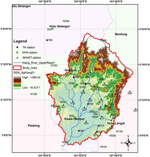
The filtering process yielded 55 rainfall stations and 55 flood events. These stations are arranged in Table 2 according to network type and location in the study area, and are denoted as an existing rainfall network. The existing rainfall network consists of the TN, NN and SMART rainfall stations, whereby TN has nine stations, SMART has 21 stations and NN has 25 stations. Forty-four (44) stations are located in the study area, and consist of eight TN stations, 17 NN stations and 19 SMART stations. The other 11 stations are located outside the study area, which consist of eight NN stations, one TN station and two SMART stations. The study area with 55 raingauge stations and three networks was mapped on the digital elevation model (DEM) of the study area, as illustrated in Figure 2.

Table 2. List of raingauge stations in the existing networks.

Station ID	Station name	Lat.	Long.	Network	Location*
T01	JPSWilayah_Tele	3.1472	101.6875	TN	In
T02	LebohPasar_Tele	3.1126	101.6966	TN	In
T03	PandanIndah_Tele	3.1274	101.7526	TN	In
T04	AirPanas_monthly_Tele	3.1887	101.7224	TN	In
T05	BktAntarabangsa_Tele	3.1837	101.7727	TN	In
T06	KgCherasBaru_Tele	3.1101	101.7474	TN	In
T07	EmpanganBatu_Tele	3.2639	101.6819	TN	In
T08	SimpangTiga_Tele	3.2453	101.7153	TN	In
N03	Km10 Ulu Kelang di UK Height	3.1947	101.7797	NN	In
N04	Jln Sg. Udang di segambut	3.1938	101.6594	NN	In
N05	Kg. Berembang di Keramat	3.1660	101.7413	NN	In
N06	JPS Wilayah Persekutuan	3.1514	101.6847	NN	In
N07	Ldg. Edinburgh Site 2	3.1833	101.6333	NN	In
N08	Klm T. Banjir Batu PO di Empat Tin	3.2467	101.6833	NN	In
N09	JPS Ampang	3.1531	101.7489	NN	In
N10	Pemasokan Ampang	3.1583	101.8014	NN	In
N14	Kg. Sg. Tua	3.2722	101.6861	NN	In
N15	Taman Ehsan di Kepong	3.2466	101.6436	NN	In
N16	Ibu Bekalan Km. 16, Gombak	3.2681	101.7292	NN	In
N17	Empangan Genting Kelang	3.2361	101.7528	NN	In
N18	Ibu Bekalan Km. 11, Gombak	3.2361	101.7139	NN	In
N19	Kg.Kuala Seleh	3.2583	101.7681	NN	In
N20	Kg. Kerdas(This station shifted from Gombak Damsite)(SMART)	3.2458	101.7153	NN	In
N21	Jam. Petaling di Jln Kelang Lama	3.0809	101.6652	NN	In
N23	Air Terjun Sg.Batu	3.3347	101.7042	NN	In
S01	SMART_Apartment UIA at Jln Gombak	3.2780	101.7280	SMART	In
S02	SMART_Bukit Ampang at Jln Ampang Hulu Langat	3.1270	101.7880	SMART	In
S03	SMART_Bulatan Kg Pandan at Jln Tun Razak	3.1400	101.7170	SMART	In
S04	SMART_DS Sg Kelang Sg Ampang Confluence	3.1660	101.7430	SMART	In
S05	SMART_IBMBS at Kg Kemensah	3.2160	101.7900	SMART	In
S08	SMART_Kuala Seleh at Empangan Kelang Gate	3.2480	101.7680	SMART	In
S09	SMART_Pusat Pengajian Luar UM at Jln Gombak	3.3250	101.75300	SMART	In
S10	SMART_Sg Ampang at Bukit Belacan	3.1430	101.7870	SMART	In
S11	SMART_Sg Ampang at Kg Melayu Ampang	3.1530	101.7610	SMART	In
S12	SMART_Sg Batu at Jln Chendurah	3.1960	101.6790	SMART	In
S13	SMART_Sg Bunus at Jln Tun Razak	3.1790	101.7120	SMART	In
S14	SMART_Sg Gombak at Jln Changkat Tmn Greenwood	3.2260	101.7080	SMART	In
S15	SMART_Sg Kerayong at Jln Kuari	3.1070	101.7430	SMART	In
S16	SMART_Sg Kelang at Empangan Kelang Gate	3.2350	101.7500	SMART	In
S17	SMART_Sg Kelang at Jln AU 5C6	3.2020	101.7590	SMART	In
S18	SMART_Sg Kelang at Jln AU 31	3.1800	101.7570	SMART	In
S19	SMART_SM Pendidikan Khas at Genting Kelang	3.2040	101.7270	SMART	In
S20	SMART_The Peak at Tmn TAR	3.1780	101.7830	SMART	In
S21	SMART_Tmn Sri Sinar	3.1860	101.6530	SMART	In
N01	Sg. Raya Bt.9 Hulu Langat	3.0678	101.7719	NN	Out
N02	Sg. Serai Bt.12 Hulu Langat	3.0994	101.7975	NN	Out
N11	Batu 14, Hulu Langat(Balai Polis)	3.1114	101.8164	NN	Out
N12	Taman Templer	3.2969	101.6328	NN	Out
N13	Kg. Melayu Sg. Buloh	3.2161	101.5761	NN	Out
N22	Ldg. Sg. Gapi	3.4003	101.6225	NN	Out
N24	Genting Sempah	3.3681	101.7708	NN	Out
N25	Taman Desa Kelisa	3.4222	101.6664	NN	Out
T09	Serendah_Tele	3.3684	101.6068	TN	Out
S06	SMART_Kem Zone 6 at Sg Congkak Resorts	3.2250	101.8390	SMART	Out
S07	SMART_Kg Pangsun at Hulu Langat	3.1760	101.8560	SMART	Out

*In: in catchment area; Out: outside catchment area.

Figure 2. Locations of raingauge stations used and a DEM of the study area.

The methodology applied involved an optimization task to select the appropriate number of raingauge stations located within the catchment area excluding the SMART stations. This was because the SMART stations were designed according to the WMO guideline for the SMART flood mitigation project. Therefore, only 25 stations remained to be evaluated, for which the rainfall data from all stations were required in the optimization task. These are the first 25 stations listed in Table 1.

Methodology

Here we present a discussion on the cross-validation technique and geostatistical method used to obtain the optimal raingauge network. First, an explanation of each method is given, followed by a detailed explanation of the proposed method application. In the proposed method, the cross-validation technique was coupled with the geostatistical method to optimize the number of raingauge stations in the raingauge network studied based on daily rainfall data.

Cross-validation

LOO and AOI cross-validation techniques

Leave-one-out (LOO) cross-validation is commonly used to evaluate the performance of variables in a dataset. It involves a simple process of leaving out a variable from the dataset temporarily and evaluating the remaining variables for their performance. This process is repeated until all variables are evaluated and a conclusion is drawn regarding their performance.

The LOO approach was employed in this study for optimization to generate a raingauge network with 25 stations. Throughout the optimization process, the intention was to remove one of the hypothetically ineffective raingauge stations at a time before being combined into the existing network (as a candidate optimum raingauge network) for evaluation based on the optimization criterion (E_rms). It was assumed that the stations omitted in each repetition were unrelated to each other to produce a better optimized network. However, every station is in fact very important in a raingauge network to produce an accurate spatial rainfall distribution. Thus, the LOO output required validation and, in order to do so, the AOI cross-validation technique was introduced.

Add-one-in (AOI) is essentially the opposite of LOO. If the LOO technique is intended to remove one station from the dataset, AOI is executed by temporarily transferring one station at a time from the dataset to be combined into the existing network (as an optimum raingauge network candidate) prior to optimization criterion evaluation. It was assumed that the added stations should remain in the optimized network. Despite both techniques having different assumptions, it is essential to evaluate the results produced by both techniques for an unbiased decision.

Geostatistical method

The geostatistical method is a well-known technique employed to study spatial or spatiotemporal datasets. It was originally developed to study mining activity (Journel and Huijbregts 1978). It is an advanced method of studying spatial datasets in vast research fields. With the geostatistical method, the datasets are modelled based on the spatial variations between each data point and presented via semi-variograms (Cheng et al. 2008, Garcia et al. 2008, Zhang and Yao 2008, Othman et al. 2011, Putthividhya and Tanaka 2012, Shaghaghian and Abedini 2013, Xu et al. 2013).

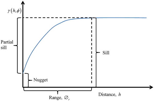
A semi-variogram is a graphical diagram that explains the relationship between the variability of a dataset and the distance of individual data in a certain direction. A typical semi-variogram example is illustrated in Figure 3. The x-axis in the diagram is a group distance between two dataset locations, also known as lag. The y-axis represents the variability measurement of the dataset group distance which is measured as semi-variance. In addition, the geostatistical characteristics of the studied dataset are inferred from the semi-variogram properties (sill, range and nugget) after fitting the studied dataset to the appropriate variogram model. In a typical semi-variogram, the nugget is the value of initial variability in the smallest group distance, including the measurement error. The variability value rises from the initial value up to the sill, where the line is off or flattened. The sill value can be read from the semi-variogram where the line is off and the partial sill is calculated by subtracting the sill from the nugget value. The range is the distance value extracted from the semi-variogram at the sill’s location on the diagram that is beyond this range and where the autocorrelation measure is zero.

Figure 3. Typical semi-variogram example.

A dataset can be modelled by:

(1)

where is the semi-variance, is the difference between the dataset pair values, is the lag (distance difference) between the dataset pair, and is the dataset size. The semi-variogram properties are calculated using a variogram model that fits the dataset.

Fitting the experimental dataset semi-variogram to the appropriate variogram model is an important stage in geostatistical analysis. There are several variogram model candidates available, but, in practice, the best model is selected to fit the experimental dataset in a semi-variogram (Ly et al. 2011, Othman et al. 2011). In a study by Othman et al. (2011), spatial rainfall analysis was conducted on the same study area as in the present study, and it was concluded that the spherical model was among the three best models, with good rainfall estimation. In our latest study (Ali and Othman 2017), we determined the best variogram model that would produce the best spatial rainfall map using the multi-criteria decision-making tool. We also found that the spherical model was the best variogram model for the study area. Therefore, the spherical model was selected in the current study to fit the experimental dataset in the semi-variogram. The spherical model is given by:

(2)

where is the semi-variance of the spherical model, C₀ is the nugget, C₁ is the sill, h is the lag (distance difference) between the dataset pair and a is the range (km). For further information on the experimental dataset fitting, the reader is referred to Ali and Othman (2017) and Journel and Huijbregts (1978).

To generate a smooth semi-variogram curve, the least squares (LS) method was adopted to fit the spherical model to the dataset. The LS method is a common method of fitting the spatial dataset to the candidate variogram model (Lee and Lahiri 2002); it employs a simple estimation of the sum squared error, E_ss, between the semi-variance of the dataset and the semi-variance estimated by the spherical model using variography properties. The aim of LS is to find the best variography property values (sill, nugget and range) of the spherical model that minimize E_ss (in Equation (3)) to produce the best semi-variogram curve. The estimated variography properties are used to calculate E_rms through the spatial interpolation method.

(3)

Spatial interpolation of rainfall

Spatial interpolation was applied to re-estimate the rainfall value at the measured point using LOO cross-validation prior to calculating E_rms. In this study, the ordinary kriging (OK) method was used to carry out spatial rainfall interpolation based on the assumption that the observed rainfall data had a constant mean but were unknown within the study area (Ali and Othman 2017).

The general equation for spatial interpolation of rainfall is:

(4)

where is the estimated rainfall value at the location and is the weighted average of the observed value . The weight is calculated based on the distance from the observed data to the predicted location and their spatial variation using the variogram model. The sum of weight must be equal to 1 to ensure that the predicted value is unbiased.

Spatial interpolation error

The optimum raingauge network was selected based on the optimization criterion, which was the E_rms value of the spatial rainfall interpolation error. The E_rms was calculated by:

(5)

where z_obs is the observed rainfall value at the raingauge, z_est is the rainfall value estimated at the raingauge through interpolation and nis the number of raingauge stations.

The E_rms value is a measurement of how close the estimated spatial rainfall value is to the observed rainfall; smaller E_rms shows that the estimation is closer to the observed value. Thus, in the optimization case, an optimum raingauge network should produce an E_rms value close to zero or the lowest compared with the other networks.

Application of the proposed optimization method

Prior to optimization, the existing raingauge network (55 stations) was divided into two datasets, containing: (1) the raingauge stations being evaluated (25 stations), denoted by R = (r₁, r₂, r₃,…, r_m); and (2) the remaining raingauge stations (30 stations) denoted by E = (e₁, e₂, e₃,…, e_n). The E dataset contains 11 stations located outside the study area. These stations are important for ensuring the continuity of the spatial interpolation of the distributed rainfall within the study area, especially at the catchment boundary. The interpolation of spatial rainfall distribution at the catchment boundary would be lost if the stations were not considered, which could increase the uncertainty and error of the rainfall distribution spatial interpolation.

Every raingauge station in each dataset contains spatial information on the longitude (x), latitude (y) and rainfall magnitude (z). A raingauge station in each dataset is denoted by:

(6)

(7)

where m and n are the numbers of stations in the datasets, while r and e are the individual stations in the datasets R and E, respectively.

The main objective of this study is to prioritize the raingauge stations in the R dataset to produce an optimum number of raingauge stations in the network. This task involves two stages of evaluation: (a) generating a candidate optimum raingauge network using the stations selected from the R dataset and combining them with the E dataset; and (b) evaluating the candidate network based on the evaluation criteria by using the spatial information (x, y, z) for each station.

In the first stage, the stations were selected through LOO and AOI cross-validation. The aim of the LOO method was to determine the stations that are less important in the optimal network. In contrast, AOI was assigned to determine the stations that are more important in the optimal network. The optimal network candidates generated by LOO and AOI were evaluated next using the geostatistical method for spatial interpolation error (E_rms) based on the variography parameters.

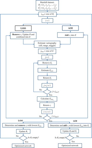
The geostatistical analysis of different network sizes produced different variography parameter values and associated spatial interpolation errors (E_rms). By manipulating this relationship, optimization was carried out to determine the optimum raingauge network for every number of raingauges selected based on the lowest E_rms. In other words, the E_rms value was set as an optimization criterion in the optimization task. The methodology employed to evaluate the optimized raingauge network in this study is summarized and presented in Figure 4.

Figure 4. Summary of methodology employed to optimize the number of raingauges in the network.

Results and discussion

Semi-variogram of existing network

Prior to optimizing a raingauge network, it is important to know the variogram properties of the existing raingauge network. For this purpose, geostatistical analysis was conducted on the existing network containing 55 raingauge stations with 55 rainfall datasets. The mean, standard deviation, variance, minimum and maximum values of the semi-variogram results are presented in Table 3.

Table 3. Descriptive statistical values of the variogram parameters of the existing network and corresponding E_rms values for selected flood events. C₁: sill; C₀: nugget; a: range; E_rms: root mean square error.

	C1	a (km)	C0	Erms
Mean	932.291	13.018	30.404	53.486
Standard deviation	632.649	8.256	59.653	173.780
Sample variance	400 244.493	68.156	3558.471	30 199.452
Minimum	179.345	3.510	2.966 × 10^–9	10.048
Maximum	3 470.901	43.943	314.026	1 284.275

Optimum raingauge network

The main objective of this study was to obtain the optimal number of raingauge stations in the network. Prior to optimizing the network, a candidate optimal network was configured by LOO and AOI cross-validation. The AOI method was introduced to re-validate the LOO method and to explore the configured candidate network for an optimal network, because the LOO method would be biased to certain rainfall datasets. Both methods produced E_rms values for every optimal network size. The raingauge network optimization results based on the E_rms value of spatial interpolation error for LOO and AOI methods were plotted against the total number of raingauge stations in the optimized network. Large rainfall datasets were used in this study, so, to demonstrate the results, seven datasets were selected to represent a sample result plot (Fig. 5).

Figure 5. Sample LOO and AOI results for E_rms against the total number of stations in the network for: (a) 3 February 2009, (b) 3 March 2009, (c) 18 September 2011, (d) 13 December 2011, (e) 7 March 2012, (f) 18 April 2012 and (g) 21 August 2012.

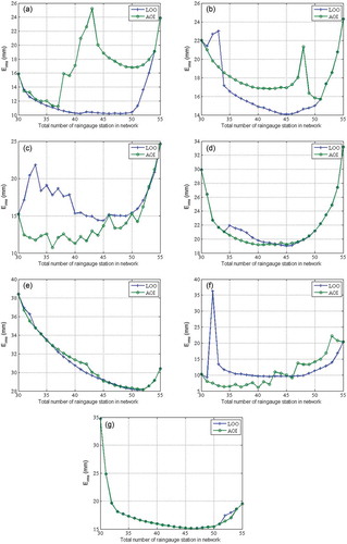
Generally, the results indicate that the E_rms value is not necessarily the lowest for the maximum or minimum number of stations in the network; in fact, lower E_rms occurred between the minimum and maximum number of stations. However, some results showed a nearly equal value of E_rms for different network sizes, as seen in Figure 5(a) for the LOO method, Figure 5(d) for the AOI method, and Figure 5(g) for both methods. Another characteristic exhibited by the results is the availability of multi-points of the minimum E_rms value, as shown in Figure 5(c) for both methods and Figure 5(f) for the AOI method. It is important to emphasize that this study was conducted based on a single-objective optimization process. Thus, the network with the lowest E_rms was selected as the best optimized network for both techniques and for each dataset. It is worth incorporating the cost in the optimization, as done by Alfonso et al. (2010), but DID information indicates that the operation and maintenance cost of each station in the study area is the same. In this case, the cost will rise with an increasing number of stations, meaning that optimal network selection will always tend toward a lower number of stations irrespective of E_rms value and despite the appearance of a lowest value. Moreover, in an optimization case, the maximum or minimum objective function value is the target.

Further assessment was carried out on the best optimized network based on the total number of stations therein (only stations inside the catchment area were considered), the subset stations selected, and the stations overlapping between LOO and AOI for their corresponding lowest E_rms values. This information was extracted and descriptive statistical analysis was carried out on the data. The descriptive statistical results are given in Table 4. As can be seen in Table 4, both methods presented similar results in terms of mean for the total number of stations in the network (35 stations), with 16 subset stations selected and an overlap of the subset stations selected (14 stations). Another similar result for both methods was the median of the total number of stations in the network (36 stations), with 17 subset stations selected and an overlap of the subset stations selected (14 stations). As for the mode of the total number of stations, the LOO method had a higher number of stations and subset stations selected (39 and 20, respectively) compared with the AOI method (36 and 17, respectively). The ranges of the numbers of stations and selected stations appeared to be slightly higher for LOO than AOI as well. Based on the descriptive statistical analysis, it was observed that AOI was more accurate in terms of average mean, median and mode values compared with LOO and had a smaller range of values for the total number of stations and subset stations selected. This observation indicates that the AOI method produced slightly better optimization results. Moreover, AOI had the lowest E_rms values for the mean and median (13.987 and 13.017, respectively).

Table 4. Descriptive statistical values of the number of raingauge stations in the optimal network for selected flood events.

	Total number of stations*		Selected subset stations		Overlap stations	Erms		Density* (km^2/station)
	LOO	AOI	LOO	AOI		LOO	AOI	LOO	AOI
Mean	35	35	16	16	14	14.702	13.987	17.4	17.1
Median	36	36	17	17	14	14.229	13.017	16.2	16.2
Mode	39	36	20	17	18	N/A	N/A	15	16.2
Minimum	19	23	0	4	0	6.562	6.795	13.9	13.9
Maximum	42	42	23	23	23	27.857	27.857	30.7	25.4

*Only stations located inside the catchment area considered.

The density of the total number of stations in the optimized network over the study area was calculated and compared with the standard set by the World Meteorological Organization (WMO). For municipal areas, the WMO standard is the range of 10–20 km² per station (WMO 2008). Based on the mean, median and mode of the density of the stations, the LOO and AOI methods met the WMO standard except for the maximum density value. This observation supports the success of the methods to optimize the existing rainfall network.

It is essential to note that the configuration of candidate networks was actually pre-determined, with 325 candidate optimal networks considered in the optimization process for each flood event. In actual application, station selection in the network configuration was based on a combinatorial case (Pardo-Igúzquiza 1998). For instance, the number of possible combinations to select a subset of stations (r) from the number of stations (N) was determined by:

(8)

The actual number of possible combinations based on the total of 25 stations ranged from 25 to 5 200 300. In geostatistical analysis, different network configurations will produce different variography structures that are used for the spatial interpolation task, which will result in different error values.

Variography structure of the optimized network

The network optimized in this study should have had a better variography structure than the existing network after optimization. To investigate this matter, the variogram properties of each best network for each dataset were extracted and compared with the existing network. The comparison of variogram properties for the existing and optimized networks with both methods in terms of mean, standard deviation and variance is illustrated in Figure 6. The mean sill value comparison in Figure 6(a) indicates little difference after the number of stations was optimized. The mean sill value of the existing network was 932.29 mm², whereas with the LOO and AOI methods the values were 913.51 and 864.06 mm², respectively. The standard deviation and variance values increased slightly with the LOO method but decreased with AOI. However, the result for the range of values was the opposite of sill for all statistical parameters. There was an increase in the range of values with both methods. The AOI method recorded the highest mean range value of 16.22 km compared to LOO with 14.83 km. As for standard deviation and variance, only the LOO method had lower values of 7.57 km and 5.73 km, respectively, compared to existing networks (8.26 km and 6.82 km, respectively). These results are due to the low number of stations configured by both methods. Thus, a lower number of stations in the raingauge network increased the value range. It also indicates that the rainfall data in the optimized network had a better correlation among stations.

Figure 6. Comparison of variogram parameter values between the existing network and network optimized by LOO and AOI: (a) sill, C₁, (b) range, a, (c) nugget, C₀, (d) E_rms, and (e) kriging variance.

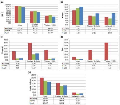
The nugget values after network optimization reduced tremendously compared with the existing network. The LOO method recorded the lowest mean nugget value of 5.02 mm, whereas AOI produced a nugget value of 5.65 mm compared with the existing network value of 30.40 mm. The rest of the statistical parameters exhibited a similar trend. Obviously, these results showed that both methods improved the variogram structure for the nugget value, especially the LOO method. Apparently, the optimized networks produced the lowest spatial interpolation error as depicted by Figure 6(d), where both methods have nearly equal values for all statistical parameters, which was the reason for nugget value improvement with both methods.

It was expected for the spatial variance of spatial rainfall interpolation to also reduce because the optimized networks had a better variography structure. To justify this observation, the mean kriging variance of spatial rainfall interpolation for the existing network and the networks optimized by LOO and AOI methods were compared, as illustrated in Figure 6(e). According to the results, the mean kriging variance value was reduced by LOO and AOI techniques more than the existing network (246.45 and 230.67, respectively). Reductions in standard deviation and kriging variance were observed as well, whereby LOO recorded lower values than AOI, with 154.44 and 23.85 × 10³, respectively.

Although the network optimized by both techniques had the lowest spatial rainfall interpolation error, better variography structures and less kriging variance of interpolation, it was important to prioritize the evaluated stations to distinguish which were classified as redundant in the network. The redundant stations could be removed in the first place to obtain an optimal network and perhaps rely on the financial constraint. Thus, a redundant station evaluation was conducted to prioritize them.

Redundant raingauge station

In raingauge network optimization, the results may depend on the type of rainfall event used. The optimized network will consist of different raingauge stations from one event to another, but there will be certain stations that appear frequently in the optimized network. In this study, the optimization task carried out using the datasets showed there were stations that overlapped frequently for every event (Table 4), which demonstrated their great importance to the network. In contrast, a few stations were incorporated in the optimized network less frequently and these can be considered redundant stations with less influence on the spatial rainfall distribution.

Therefore, to prioritize the hypothetical redundant stations selected for the optimized network using the two methods with 55 flood events, the frequency rate (F_r) was calculated by dividing the station frequency by the total number of flood events. The F_r value signifies the station’s importance to remain in the raingauge network and a redundant station should have a lower F_r value. The F_r values were in the [0,1] range and were sorted in descending order, as seen in Table 5. To evaluate the redundant stations, the threshold F_r value of 0.5 was first set to benchmark the redundant stations. Those stations with F_r values below 0.5 were deemed less important. Then the stations in this category were compared between the two methods.

Table 5. Frequency of subset stations chosen in the optimized raingauge network.

LOO method		AOI method
Station	Fr	Station	Fr
N04	0.819	T05	0.837
T05	0.746	N05	0.782
N14	0.746	N19	0.782
N18	0.746	N04	0.764
N05	0.728	N16	0.764
N16	0.728	N10	0.746
N10	0.71	N09	0.728
N09	0.691	N17	0.710
N19	0.691	T03	0.673
T03	0.673	N14	0.673
N17	0.673	N18	0.673
T07	0.600	T08	0.619
T08	0.600	N07	0.619
N20	0.600	T04	0.582
N23	0.600	T06	0.582
T01	0.582	N23	0.582
N06	0.582	N08	0.564
N07	0.582	N15	0.564
T06	0.564	N03	0.546
N08	0.564	N20	0.546
N15	0.564	T01	0.510
T04	0.528	T07	0.510
T02	0.510	N06	0.491
N03	0.473	N21	0.491
N21	0.455	T02	0.419

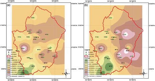
Based on the results, the LOO method showed two stations below the threshold value, while AOI resulted in three stations. Those stations were compared with the stations overlapping at the threshold F_r value and only one more station, N21, made a total of four stations (N03, N06, N21 and T02) at the threshold value. These four stations were inferred to be ineffective and were classified as redundant stations. Spatial analysis indicates that three stations (N06, N21 and T02) were located at the southwest of the study area and one station was located in the eastern area. In the southwestern area, the stations were sparse both in the study area and outside. Sparse rainfall stations normally affect the spatial rainfall interpolation accuracy; hence, these stations were likely ineffective. In addition, station N06 was redundant with another station, T1, which was located at a distance of 557 m. In contrast, station N03 was surrounded by four stations in the east, making N03 less important to spatial rainfall interpolation. For this reason, it would be good to relocate N03 and N06 to the southwest to enhance the sparse stations in this area. This is an improvement opportunity to be explored in future studies since it was not included in the scope of this study. The F_r values are plotted in Figure 7 for a better representations of which stations are often selected in an optimized network.

Figure 7. Frequency rate (F_r) map of stations remaining in the optimal network: (a) optimized by LOO and (b) optimized by AOI.

The four redundant stations were also evaluated using the variability of received rainfall along the available records, measured as the probability of zero rainfall calculated by , where is the probability of wet days on which the station recorded non-zero rainfall values. This evaluation was adopted from Yoo et al. (2008), who used it in their study to compare the application of mixed and continuous distribution functions to the entropy theory for raingauge network evaluation. However, we adopted the probability of zero rainfall to validate the selection of redundant stations based on a higher probability of zero rainfall values. For this purpose, long-term daily records of non-zero rainfall were counted along the duration of the stations’ existence and divided by the total duration. A probability value of zero rainfall indicates the location’s efficiency to gauge rainfall.

Among the four stations, T02 had a higher P value of 0.52, and N06 and N21 had equal P values of 0.5; meanwhile, N03 had a P value of 0.45. Based on these results, three stations are moderately important for gauging long-term rainfall. However, N03 indicated slight efficiency in gauging rainfall.

Optimal network performance in simulating flood events

The optimal network without the four redundant stations was preliminarily evaluated to simulate the flood events used in the optimization process. The network should be able to simulate the flood events with a more satisfactory level of model efficiency than the existing network. For this purpose, the modified hydrological tank model (MHTM) of the DID was used to simulate floods at stations located downstream of the catchment area near station N21.

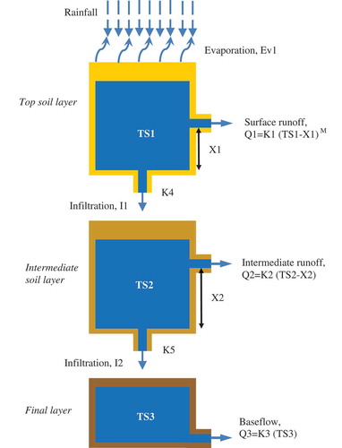
The MHTM was set up using three tanks organized in vertical order, as depicted in Figure 8. The top tank represented the top soil layer with rainfall as an input. It modelled the hydrological processes in this layer consisting of rainfall, surface evaporation, infiltration into the next soil layer, storage volume, maximum storage depth and surface runoff. The subsequent tank represented the intermediate soil layer. Infiltration from the top tank was the main input to the tank’s storage. This tank modelled the interaction between the input and intermediate runoff as well as infiltration that percolated into the last tank by considering the tank storage and storage depth. The last tank represented the baseflow generated by infiltration from the intermediate tank and available storage without further infiltration. The combination of surface runoff, intermediate flow and baseflow is the total flow of the river basin. The MHTM has 12 parameters involved in the hydrological process to produce the total flow of the river basin from rainfall, as tabulated in Table 6.

Table 6. Tank model parameters in the calibration process.

Parameter	Description
TS1	Storage coefficient of Tank 1
TS2	Storage coefficient of Tank 2
TS3	Storage coefficient of Tank 3
Ev1	Evaporation of water body in Tank 1
M	Storage power coefficient to calculate the direct runoff in Tank 1
X1	Level of storage in Tank 1 just before Q1 generation
X2	Level of storage in Tank 2 just before Q2 generation
K1	Runoff coefficient of Tank 1
K2	Runoff coefficient of Tank 2
K3	Runoff coefficient of Tank 3
K4	Infiltration coefficient of infiltration occurring from Tank 1
K5	Infiltration coefficient of infiltration occurring from Tank 2

Figure 8. Tank model set-up by DID for the study area.

The MHTM was calibrated and validated using an automatic calibration approach, i.e. particle swarm optimization. The 12 parameters were calibrated using 25 swarm particles for 1000 iterations. The areal rainfall data series for the 15-min interval served as input data to the model, and the Thiessen polygon method was used to calculate the areal rainfall of the raingauge network. For the purpose of this study, six datasets (3 February 2009, 3 March 2009, 18 September 2011, 7 March 2012, 18 April 2012 and 21 August 2012) were selected to demonstrate the performance of the optimized rainfall network. The rainfall data series was simulated to produce the flow at the calibration point located at the final outlet of the river basin near station N21 for two conditions: simulation using the existing network and without the four redundant stations. The Nash-Sutcliffe efficiency (NSE) criterion was used to measure the model efficiency and the results were compared to evaluate the optimal network performance in generating an accurate historical flood hydrograph.

The NSE values of the simulation results are given in Table 7. Four samples recorded NSE values over 0.75, which are efficient enough to simulate a flood hydrograph, thus justifying the optimal network selection with the proposed method. However, the two datasets for 3 February 2009 and 7 March 2012 did not show good results, with NSE below 0.75. For these datasets, the four redundant stations deteriorated the model efficiency. These datasets recorded high absolute error (AE) values of 97.99 and 56.7%, respectively. These results are possibly due to the characteristics of the rainfall events (e.g. convective or stratified), which are not included in the scope of this study. Nonetheless, the model can be improved by re-calibrating it with the optimal rainfall network, as concluded by Bárdossy and Das (2008).

Table 7. Preliminary comparison of NSE values of the existing and the optimal networks. NSE: Nash Sutcliffe Efficiency; AE: absolute error.

Flood event	NSE	Optimal network	AE (%)
	Existing network
3 February 2009	0.9945	0.0200	97.99
3 March 2009	0.9959	0.7831	21.36
18 September 2011	0.9937	0.9916	0.21
7 March 2012	0.7494	0.3245	56.70
18 April 2012	0.9958	0.9550	4.10
21 August 2012	0.9952	0.9376	5.79

Conclusion

In this study, an optimization process was developed by coupling cross-validation with geostatistical analysis to prioritize the raingauge stations in a network through optimization. The method was applied to optimize the number of stations in a raingauge network in a tropical urban area. The total daily rainfall data from 55 raingauge stations were used to perform the optimization process for 55 flood events. The aim of optimization was to reduce the number of raingauge stations in the existing network that were hypothetically redundant.

Four important points from this study are summarized as follows:

1. By coupling the cross-validation technique with geostatistical analysis, the number of stations in the existing raingauge network could be optimized based on the lowest E_rms value of spatial interpolation error with two different approaches of raingauge network configuration (LOO and AOI). However, at the lowest E_rms value, both approaches resulted in different total numbers of stations in the optimized raingauge network.

2. By coupling the cross-validation technique with geostatistical analysis, the number of stations in the existing raingauge network could be optimized based on the lowest E_rms value of spatial interpolation error with two different approaches of raingauge network configuration (LOO and AOI). However, at the lowest E_rms value, both approaches resulted in different total numbers of stations in the optimized raingauge network.

3. By coupling the cross-validation technique with geostatistical analysis, the number of stations in the existing raingauge network could be optimized based on the lowest E_rms value of spatial interpolation error with two different approaches of raingauge network configuration (LOO and AOI). However, at the lowest E_rms value, both approaches resulted in different total numbers of stations in the optimized raingauge network.

4. By coupling the cross-validation technique with geostatistical analysis, the number of stations in the existing raingauge network could be optimized based on the lowest E_rms value of spatial interpolation error with two different approaches of raingauge network configuration (LOO and AOI). However, at the lowest E_rms value, both approaches resulted in different total numbers of stations in the optimized raingauge network.

By coupling the cross-validation technique with geostatistical analysis, the number of stations in the existing raingauge network could be optimized based on the lowest E_rms value of spatial interpolation error with two different approaches of raingauge network configuration (LOO and AOI). However, at the lowest E_rms value, both approaches resulted in different total numbers of stations in the optimized raingauge network.

Generally, the optimized raingauge network exhibited a better semi-variogram structure and lower spatial interpolation error. Both optimization methods demonstrated a drastic improvement in nugget value and E_rms value. The LOO method showed a slightly better nugget value, while the AOI method showed a slightly better result for the E_rms and kriging variance values.

In the study area, the raingauge stations were prioritized based on their importance in the network. Four stations (T02, N03, N06 and N21) were considered ineffective and could therefore be relocated within the study area or eliminated from the existing network.

A preliminary evaluation of the optimized network without the four stations showed satisfactory results in flood simulation using a lumped hydrological model.

An essential task in this study was to configure the optimized network with the existing stations. The selection of subset stations in the existing network was similar to the combinatorial case, where all combinations were to be examined to find the best one. To improve the current study results, this matter should be addressed in an upcoming study using particle swarm optimization to optimize the existing raingauge network. In addition, the proposed method of application will be extended with the use of finer time intervals of rainfall data.

Acknowledgements

The authors would like to thank the Drainage and Irrigation Department of Malaysia (DID) for providing the hydrological data and supportive co-operation. We would also like to thank the Water Research Centre of the University of Malaya for their support and assistance. We are most grateful and would like to thank the reviewers for their valuable suggestions, which have led to a substantial improvement of the article.

Disclosure statement

No potential conflict of interest was reported by the authors.

Additional information

Funding

This work was supported by the University of Malaya Research Grant [Grant number FL001-13SUS and RP017C-15SUS].

References

- Adhikary, S.K., Yilmaz, A.G., and Muttil, N., 2015. Optimal design of raingauge network in the Middle Yarra River catchment, Australia. Hydrological Processes, 29 (11), 2582–2599. doi:10.1002/hyp.v29.11
- Alfonso, L., et al. 2014. Ensemble entropy for monitoring network design. Entropy, 16 (3), 1365–1375. doi:10.3390/e16031365
- Alfonso, L., Lobbrecht, A., and Price, R., 2010. Optimization of water level monitoring network in polder systems using information theory. Water Resources Research, 46 (12), n/a-n/a. doi:10.1029/2009WR008953
- Ali, M.Z.M. and Othman, F., 2017. Selection of variogram model for spatial rainfall mapping using analytical hierarchy procedure (AHP). Scientia Iranica, 24 (1), 28–39. doi:10.24200/sci.2017.2374
- Awadallah, A.G., 2012. Selecting optimum locations of rainfall stations using kriging and entropy. International Journal of Civil & Environmental Engineering IJCEE, 12, 36–41.
- Barca, E., Passarella, G., and Uricchio, V., 2008. Optimal extension of the raingauge monitoring network of the Apulian Regional Consortium for Crop Protection. Environmental Monitoring and Assessment, 145 (1–3), 375–386. doi:10.1007/s10661-007-0046-z
- Bárdossy, A. and Das, T., 2008. Influence of rainfall observation network on model calibration and application. Hydrology and Earth System Sciences, 12 (1), 77–89. doi:10.5194/hess-12-77-2008
- Bastin, G., et al. 1984. Optimal estimation of the average areal rainfall and optimal selection of raingauge locations. Water Resources Research, 20, 463–470. doi:10.1029/WR020i004p00463
- Chen, Y.-C., Wei, C., and Yeh, H.-C., 2008. Rainfall network design using kriging and entropy. Hydrological Processes, 22 (3), 340–346. doi:10.1002/(ISSN)1099-1085
- Cheng, K.S., Lin, Y.C., and Liou, J.J., 2008. Rain‐gauge network evaluation and augmentation using geostatistics. Hydrological Processes, 22 (14), 2554–2564. doi:10.1002/hyp.6851
- Feki, H., Slimani, M., and Cudennec, C., 2016. Geostatistically based optimization of a rainfall monitoring network extension: case of the climatically heterogeneous Tunisia. Hydrology Research, 48, 6. doi:10.2166/nh.2016.256
- Garcia, M., Peters-Lidard, C.D., and Goodrich, D.C., 2008. Spatial interpolation of precipitation in a dense gauge network for monsoon storm events in the southwestern United States. Water Resources Research, 44 (5), n/a-n/a. doi:10.1029/2006WR005788
- Journel, A.G. and Huijbregts, C.J., 1978. Mining geostatistics. New York: Academic Press.
- Jung, Y., et al. 2014. Rain-gauge network evaluations using spatiotemporal correlation structure for semi-mountainous regions. Terrestrial Atmospheric and Oceanic Sciences, 25 (2), 267–278. doi:10.3319/TAO.2013.10.31.01(Hy)
- Kamel, H.F.E., Slimani, M., and Cudennec, C., 2010. A comparison of three geostatistical procedures for rainfall network optimization. Sousse, Tunisia: International Renewable Energy Congress, 260–267.
- Kar, A.K., et al. 2015. Raingauge network design for flood forecasting using multi-criteria decision analysis and clustering techniques in lower Mahanadi river basin, India. Journal of Hydrology. Regional Studies, 4, 313–332.
- Krstanovic, P.F. and Singh, V.P., 1992a. Evaluation of rainfall networks using entropy: I. Theoretical Development. Water Resources Management, 6, 279–293. doi:10.1007/BF00872281
- Krstanovic, P.F. and Singh, V.P., 1992b. Evaluation of rainfall networks using entropy: II. Application. Water Resources Management, 6, 295–314.
- Lee, Y.D. and Lahiri, S.N., 2002. Least squares variogram fitting by spatial subsampling. Journal of the Royal Statistical Society. Series B (Statistical Methodology), 64 (4), 837–854. doi:10.1111/1467-9868.00364
- Li, C., Singh, V.P., and Mishra, A.K., 2012. Entropy theory-based criterion for hydrometric network evaluation and design: maximum information minimum redundancy. Water Resources Research, 48 (5), n/a-n/a. doi:10.1029/2011WR011251
- Ly, S., Charles, C., and Degré, A., 2011. Geostatistical interpolation of daily rainfall at catchment scale: the use of several variogram models in the Ourthe and Ambleve catchments, Belgium. Hydrology and Earth System Sciences, 15 (7), 2259–2274. doi:10.5194/hess-15-2259-2011
- Mishra, A.K. and Coulibaly, P., 2010. Hydrometric network evaluation for Canadian watersheds. Journal of Hydrology, 380 (3–4), 420–437. doi:10.1016/j.jhydrol.2009.11.015
- Mishra, A.K. and Coulibaly, P., 2014. Variability in Canadian seasonal streamflow information and its implication for hydrometric network design. Journal of Hydrologic Engineering, 19 (8), 05014003. doi:10.1061/(ASCE)HE.1943-5584.0000971
- Nemec, J. and Askew, A.J., 1986. Mean and variance in network-design philosophies. In: M.E. Moss, ed. Integrated design of hydrological networks. Proceedings of the Budapest Symposium, July 1986. Wallingford, UK: International Association of Hydrological Sciences, IAHS Publ. 158, 123–131. Available from: https://iahs.info/uploads/dms/iahs_158_0123.pdf [Accessed 1 Feb 2018].
- Othman, F., Akbari, A., and Samah, A.A., 2011. Spatial rainfall analysis for an urbanized tropical river basin. International Journal of the Physical Sciences, 6 (20), 4861–4868.
- Pardo-Igúzquiza, E., 1998. Optimal selection of number and location of rainfall gauges for areal rainfall estimation using geostatistics and simulated annealing. Journal of Hydrology, 210, 206–220. doi:10.1016/S0022-1694(98)00188-7
- Putthividhya, A. and Tanaka, K., 2012. Optimal raingauge network design and spatial precipitation mapping based on geostatistical analysis from colocated elevation and humidity data. International Journal of Environmental Science and Development, 3, 2.
- Ridolfi, E., et al. 2011. An entropy approach for evaluating the maximum information content achievable by an urban rainfall network. Natural Hazards and Earth System Science, 11 (7), 2075–2083. doi:10.5194/nhess-11-2075-2011
- Ridolfi, E., et al. 2012. An entropy method for floodplain monitoring network design. AIP Conference Proceedings, 1479, 1780–1783.
- Shaghaghian, M.R. and Abedini, M.J., 2013. Raingauge network design using coupled geostatistical and multivariate techniques. Scientia Iranica, 20 (2), 259–269.
- Shannon, C.E. and Weaver, W., 1949. The mathematical theory of communication. Urbana: University of Illinois Press.
- Şorman, Ü. and Balkan, G., 1983. An application of network design procedures for redesigning Kizilirmak River basin raingauge network, Turkey. Hydrological Sciences Journal, 28 (2), 233–246. doi:10.1080/02626668309491963
- Vivekanandan, N. and Jagtap, R.S., 2013. Review and analysis of stream gauge and raingauge networks using spatial regression approach. WYNO Journal of Engineering & Technology Research, 1 (2), 10–21.
- Vivekanandan, N., Roy, S., and Chavan, A., 2012. Evaluation of raingauge network using maximum information minimum redundancy theory. International Journal of Scientific Research and Reviews, 1 (3), 96–107.
- Volkmann, T.H.M., et al. 2010. Multicriteria design of raingauge networks for flash flood prediction in semiarid catchments with complex terrain. Water Resources Research, 46, 11. doi:10.1029/2010WR009145
- Wei, C., et al. 2010. Raingauges network design using discrete entropy and kriging. In: EGU General Assembly 2010, 2–7 May, Vienna, Austria. Geophysical Research Abstracts, 12 (EGU2010-10421).
- WMO (World Meteorological Organization), 2008. Guide to hydrological practices. Volume I (Hydrology – from measurement to hydrological information). 6th ed. Geneva, Switzerland: World Meteorological Organization.
- Xu, H., et al. 2013. Assessing the influence of raingauge density and distribution on hydrological model performance in a humid region of China. Journal of Hydrology, 505, 1–12. doi:10.1016/j.jhydrol.2013.09.004
- Xu, H., et al. 2015. Entropy theory based multi-criteria resampling of raingauge networks for hydrological modelling – A case study of humid area in southern China. Journal of Hydrology, 525, 138–151. doi:10.1016/j.jhydrol.2015.03.034
- Yeasmin, D. and Pasha, M.F.K., 2008. Runoff prediction by GIS using optimal number of raingauges. Honolulu, HI: World Environmental and Water Resources Congress. Ahupua’a.
- Yeh, H.-C., et al. 2011. Entropy and kriging approach to rainfall network design. Paddy and Water Environment, 9 (3), 343–355. doi:10.1007/s10333-010-0247-x
- Yoo, C., Jung, K., and Lee, J., 2008. Evaluation of raingauge network using entropy theory: comparison of mixed and continuous distribution function applications. Journal of Hydrologic Engineering, 13, 226–235. doi:10.1061/(ASCE)1084-0699(2008)13:4(226)
- Zhang, J. and Yao, N., 2008. The geostatistical framework for spatial prediction. Geo-Spatial Information Science, 11 (3), 180–185. doi:10.1007/s11806-008-0087-7