A new method for establishing hydrologic fidelity of snow depth measurements based on snowmelt–runoff hydrographs

ABSTRACT

For snowmelt-driven flood studies, snow water equivalent (SWE) is frequently estimated using snow depth data. Accurate measurements of snow depth are important in providing data for continuous hydrologic simulations of such watersheds. A new hydrologic fidelity metric is proposed in this study to evaluate the potential contribution of particular snow depth datasets to flow characteristics using observed data and hydrologic modeling using the Variable Infiltration Capacity (VIC) model. Data-based hydrologic fidelity of snow depth measurements is defined as a categorical skill score between the snow depth in the watershed and the hydrograph peak or volume at the watershed outlet. Similarly, model-based hydrologic fidelity is defined as a categorical skill score between the model-simulated snow depth and the model-simulated hydrograph peak or volume. The proposed framework is illustrated using the Pecatonica River watershed in the USA, indicating which sites have a higher hydrologic fidelity, which is preferred in hydrologic studies.

KEYWORDS:

• Barnstone skill score
• Gerrity skill score
• LEPS skill score
• VIC model
• snow depth
• snow gauge evaluation

Editor A. Castellarin Associate editor G. Thirel

Introduction

As a part of the Federal Emergency Management Agency map modernization effort, a restudy of the Pecatonica River in Illinois and Wisconsin, located approximately 100 km west of the Chicago and Milwaukee metropolitan areas, has been performed to account for a more complete set of hydrologic data. This river, along with several other streams and rivers in the region, also called the Wisconsin Driftless area, has exhibited a significant decreasing trend in annual peak flows. Although the restudy accounted for the trend (Markus et al. 2013), the causes of the trends were not fully explained. The researchers attributed these trends to the adoption of various measures for soil and water conservation (Potter 1991, Kochendorfer and Hubbart 2010), drainage improvement (Gebert and Krug 1996) or climate change combined with land-use changes (Juckem et al. 2008, Markus et al. 2013). To assess the contribution of climate change to the decreasing snowmelt late winter peaks in the Pecatonica River, Park and Markus (2014) developed an application of the Variable Infiltration Capacity (VIC) model (Andreadis et al. 2009, Sinha and Cherkauer 2010, Sinha et al. 2010, Tan et al. 2011) in two different modes: the event mode and the continuous mode. Markus et al. (2013) evaluated the snow gage records collected by the National Climatic Data Center (NCDC) of the NOAA (US National Oceanic and Atmospheric Administration) and stored in the Midwestern Regional Climate Center (MRCC) database. In particular, they reviewed the recent climate data quality report published by Kunkel et al. (2009). During this review, it was observed that the gages which are deemed reliable for climate studies were not always as useful in hydrologic modeling, and vice versa. The inconsistency between the NCDC station reliability for climate-related studies and its usability for hydrologicstudies prompted this study, in which we designed a new measure of hydrologicusability of snow depth data. This measure is defined through a categorical correspondence between each snow gage and the peak and volume of the corresponding snowmelt hydrograph. The degree of this correspondence is referred to as the hydrologic fidelity of snow gages. A similar term was previously used by Mobley et al. (2012), who defined “precipitation fidelity” as a measure of correspondence between the estimated precipitation and stream outflow in rainfall–runoff processes. The fidelity defined in this paper, however, focuses on snowmelt–runoff flood events, and is applicable to watersheds with dominant snow-driven hydrologic processes.

Snow depth monitoring is critical in various hydrologic trend and variability studies, frequency analysis, and real-time flood forecasting for watersheds with snowmelt-driven regimes (Jonas et al. 2009, Jörg-Hess et al. 2014). However, typical quality-control procedures for snow depth observed records (e.g. Kunkel et al. 2009, Jörg-Hess et al. 2014) do not include their hydrologic usability. To address this issue we have developed a framework to determine hydrologicfidelity of snow measurements (hereafter referred to as the “hydrologic fidelity”). Hydrologic fidelity is defined as a categorical correspondence between the observed snow depth and the observed river flow. Many researchers (Freeze and Harlan 1969, Kirnbauer et al. 1994, Jasper and Kaufmann 2003, Zappa 2008) used some simple categorical statistics based on 2 × 2 contingency tables for hydrology fields; this study applied the more comprehensive categorical statistics of 4 × 4 contingency tables for estimating the hydrologic fidelity. It was calculated for a number of snowmelt events in the Pecatonica River watershed. This river is particularly significant due to its pronounced decreasing trend in annual peak flows (Potter 1991, Gebert and Krug 1996, Juckem et al. 2008, Kochendorfer and Hubbart 2010, Markus et al. 2013).

Hydrologic fidelity calculated as a categorical correspondence between the observed snow depth and the observed river flow is referred to as the data-based hydrologic fidelity. Similarly, the model-based hydrologic fidelity is determined as a categorical correspondence between the model-generated snow depth and the model-generated river flow. The model-based analyses were performed using the Variable Infiltration Capacity (VIC) model (Liang et al. 1994, 1996, Andreadis et al. 2009, Sinha and Cherkauer 2010, Sinha et al. 2010, Tan et al. 2011). This study applied the VIC model to compare the results of the observed snow depth and flow characteristics. The VIC model is a land-surface simulation model based on water balance and energy balance. It should be noted that this framework could use any other snowmelt–runoff model such as SNOW17 (Anderson 1973), which was recently applied to provide improved discharge simulations using an ensemble Kalman filter to snow water equivalent assimilation in the Pecatonica River basin (Dziubanski and Franz 2016). Both data- and model-based hydrologic fidelities provide useful information about the benefits of these gages in hydrologic studies, which can be used to evaluate climate monitoring networks.

Methods and data

Categorical skill scores

The strength of association between two variables in hydrology has been evaluated using numerous methods, such as the Pearson correlation coefficient, root mean square error (RMSE), Nash-Sutcliffe efficiency index (NSEI), and various categorical skill score matrices. Many researchers have studied and compared these evaluation methods. Markus et al. (2010) showed that model evaluation can depend on the choice of the evaluation methods and suggested a multi-model multi-tool evaluation matrix. Barnston (1992) argued in favor of categorical skill scores over the correlation coefficient, particularly when the relationship is nonlinear.

Many categorical skill score methods, such as the false alarm ratio (Haklander and Van Delden 2003), the critical success index (Roebber et al. 2002), the Heidke skill score (Benedetti et al. 2005), and the categorical bias (Eder et al. 2006), consider only diagonal entries in a contingency table. These methods typically assign zero weights to all the off-diagonal elements, regardless of how close to the diagonal they are, which can be problematic for 3-by-3 and higher order matrices (Ward and Folland 1991, Gandin and Murphy 1992, Rodwell et al. 2010). For this reason, various weight matrices have been suggested to evaluate multi-contingency tables based on probabilistic score estimation, generally referred to as “equitable skill scores.” Gandin and Murphy (1992) suggested basic principles to develop equitable skill scores, described the derivation of a three-category skill score matrix, and suggested conditions for multi-categorical skill scores. This method assigns the maximum value of 1 to a perfect skill and the value of 0 for no skill. Gerrity (1992) further developed the score calculation by Gandin and Murphy and suggested general equations to produce multi-category equitable skill scores. The value of the Gerrity skill score (GSS) for a categorical forecast with K categories is as follows (Gerrity 1992, Livezey 2012, Yossef et al. 2012):

(1)

where p_ij is the relative sample frequency and s_ij is the corresponding scoring factor from skill score matrix S. The elements of a K × K equitable scoring matrix may be written as:

(2)

(3)

(4)

where .

It is assumed that the skill score matrix S is symmetric, as shown by (Gerrity 1992):

(5)

The term a_i is the ratio of the probability that an observation falls into a class with an index greater than i to the probability that it falls into a class with an index as follows:

(6)

where p_r < 1 is the frequency with which class r of the event is observed. In this study, all p_r values are assumed equal to 1/K equivalently for K × K equitable scoring matrices. For example, for a 4 × 4 equitable matrix, all p_r values are equal to 0.25, as represented in Table 1(a).

Table 1. Four-category skill score matrices used in this study.

Method	(a) Gerrity skill score	(b) LEPS skill score	(c) Barnston skill score
Matrix of parameters

Ward and Folland (1991) suggested a new normalization method named the linear error in probability space (LEPS) score, as shown in Table 1(b). The LEPS score is based on the linear distance between the forecast and the observation in their sample probability spaces. The LEPS score (Sʺ) is defined as:

(7)

where P_f and P_o are, respectively, the forecast and observed cumulative probabilities from the nonexceedence curve (Potts et al. 1996). Barnston (1992) presented modified categorical LEPS scores incorporating a credit/penalty scoring system for two to five categories (Table 1(b)). The LEPS score is expected to be less sensitive to skill trends and more vulnerable to hedging than the GSS, but more able to differentiate between good and bad forecasts (Livezey 2012). Barnston (1992) also developed a modified Heidke skill score, herein referred to as the Barnston skill score, in which the penalty for an incorrect forecast was linearly dependent on the class of the category error; a 4 × 4 equitable matrix is represented in Table 1(c).

This study utilizes four-category contingency tables for the Barnston, LEPS, and Gerrity equitable skill scores, as shown in Table 1. All of the skill scores used herein contain the following relationships:

(8)

(9)

where p_i and p_j are the forecast event probabilities and . This study assumes that p_i and p_j are equivalent to 1/K.

The categorical skill score 4 × 4 matrices are used herein to evaluate statistical associations between snow depth and river discharge for a set of snowmelt–runoff events. In this research, the datasets for which the categorical skill score is being evaluated are each divided into four groups separated by the three quartiles (25th, 50th, and 75th percentiles). For example, for data-based fidelity, the categorical correspondence is calculated between the observed snow depths and the observed hydrograph peaks (or volumes). If, for each point, the predictor and the predictand fall into the same group, the resulting skill score matrix will have all off-diagonal elements equal to zero. Conversely, the matrix will have non-zero off-diagonal elements if the predictor and predictand for at least one data point do not fall into the same group.

VIC model

The VIC (variable infiltration capacity) model (Liang et al. 1994, 1996, Andreadis et al. 2009, Sinha and Cherkauer 2010, Sinha et al. 2010, Tan et al. 2011) is a grid-based land surface model that simulates water balance and energy balance. Accordingly, the VIC model can simulate various meteorological, hydrological, and soil variables. The original VIC model was a two-layer model (Liang et al. 1994), but Liang et al. (1996) found that a three-layer VIC model produced more accurate results. The VIC model has since been improved with an upgraded energy balance module (Andreadis et al. 2009), frozen soil algorithm (Cherkauer and Lettenmaier 1999, 2003, Cherkauer et al. 2003), and blowing snow algorithm (Bowling et al. 2004). The VIC model can also estimate snow property variables such as snow depth, sublimation, SWE (snow water equivalent), and snowmelt, and can calculate snowmelt-driven streamflow using these variables. In particular, the VIC model calculates energy and mass balance of the snowpack, similar to other methods for cold land process described in Anderson (1976), Wigmosta et al. (1994), and Tarboton et al. (1994). Andreadis et al. (2009) describe the detailed energy balance process for the surface layer of the VIC model. The routing scheme for both grid cell and river routing are built as simple linear transfer functions. It is assumed that the runoff transport is linear, causal, stable, and time invariant (Lohmann et al. 1996, 1998).

Watershed data

The Pecatonica River watershed is located in southern Wisconsin and northern Illinois, USA (Fig. 1). It has a drainage area of 3435 km², which is predominantly agricultural and forested land. The watershed is located approximately 100 km west of Lake Michigan, near the two large coastal metropolitan areas of Milwaukee and Chicago. The Pecatonica River watershed varies in elevation from 219 to 357 m a.s.l. The hydrology of the Pecatonica River project area is “driven by local climate conditions and the landscape, consisting of rolling hills and well developed stream valleys” (IDNR 1998).

Figure 1. Pecatonica watershed map (adopted from Park and Markus 2014).

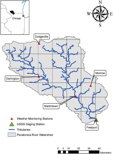
Five climate stations operated by the NCDC were selected to provide snow data: Dodgeville, Darlington, Martintown, and Monroe in Wisconsin, and Freeport in Illinois. At these stations, the observed data include daily snow depth measurements between 1915 and 2014. In this area, the snowfall season typically occurs between December and March, and the snowpack typically melts in February and March (Park and Markus 2014). Temperatures range between −30°C in the winter and +30°C in the summer, and the growing season generally stretches from May to September. Average annual precipitation is around 800 mm. (Juckem et al. 2008). Daily streamflow data (1915–2014) were recorded at the US Geological Survey (USGS) gaging station for the Pecatonica River in Freeport, Illinois (USGS no. 05435500). Although this USGS station has been moved several times, it was assumed that the uncertainty of flow measurements is much smaller than that of snow depth observations. Thus, in this study, for the snowmelt–runoff process, the snow observations correlating with flow observation were considered more accurate than those with poorer correlations.

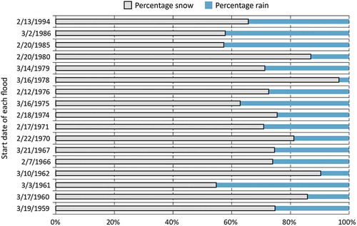
In the Pecatonica River watershed, snowmelt-dominated flood events typically occur in February or March. These flood events are types of rain-on-snow events, which have been studied by many researchers (Harr 1986, Marks et al. 1998, McCabe et al. 2007). We started with a selection of the 23 largest historical flood events observed in February or March where snow depth data were available at all five climate stations between 1959 and 1994. Then, among the largest historical flood events, we excluded six events in which the rainfall was greater than 50%, further reducing the number of events to 17. The selected 17 events are visualized in Figure 2 through a snow volumetric contribution for each event, defined herein as SWE/(SWE+R), where SWE stands for snow water equivalent melted during the event and R for rainfall observed during the event. A traditional snow-to-liquid ratio of 10 was selected. More information on the relationship between snowfall/snowpack and liquid water equivalent in this region can be found in Baxter et al. (2005). The volumetric contribution of snow to these events was on average 74% (Fig. 2).

Figure 2. Volumetric percentage of snow and rain contributing to each flood event at Freeport on the Pecatonica River (USGS no. 05435500).

Snow depth measurements

There are numerous publications on hydrometric networks, generally focusing on streamgaging or raingaging networks. A comprehensive review of hydrometric networks is provided by Mishra and Coulibaly (2009). Snowfall and snowpack depth in the Western United States (SNOTEL network, http://www.wcc.nrcs.usda.gov/snow/) is highly critical for water supply and varies significantly by elevation, warranting a denser network than would be required in other parts such as the Midwest. The depth measurement data in this study were subject to quality control and assurance similar to those described in Kunkel et al. (2009). These procedures are conducted at the MRCC in Champaign, Illinois.

The present snow depth measurements in the Pecatonica River watershed were made following the standards described in the NOAA manual (http://www.nws.noaa.gov/om/coop/reference/Snow_Measurement_Guidelines.pdf). Snow on the ground measurements include the new 24-hour snowfall and the snow that has accumulated from previous days. These measurements are made with a measuring stick at several locations where the snow cover has not been disturbed, followed by an averaging. The early snow depth records were based on the US Weather Bureau 1915 (Instructions for Cooperative Observers, US Weather Bureau, Instrument Division Circular B and C 5th edition. W.B. 539). The following statement in the report describes the method: “Select a level place of some extent, where the drifting is least pronounced, and measure the snow in at least three places.”

VIC model calibration

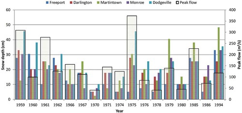
In the Pecatonica River watershed, late winter snowmelt-driven floods have been larger than rainfall-driven floods in spring and summer. As the available climate (precipitation, minimum temperature, maximum temperature, and snow depth) and hydrologic data (river flows) have a daily time step, the event-based model simulations also had an increment of 1 day. The grid cell size was 1/8° × 1/8°. In order to validate the data-based and model-based fidelities of snow gages in the watershed, the largest snowmelt-driven floods observed at the outlet of this watershed were selected (Fig. 3). Large snow depths prior to the flood event generally correlate with large peak flows. However, there is a considerable variability in this correlation, due to numerous factors including variable rainfall contribution for each event, and a limited ability of discrete observed snow depths to represent the continuous SWE accurately.

Figure 3. Observed snow depths (colors) at the beginning of each flood event at five climate gages and the corresponding flood peaks (wide boxes with black borders) at Freeport on the Pecatonica River for 17 selected snowmelt-driven floods.

Soil and land cover parameters needed for VIC model calibration were acquired from the Land Data Assimilation System (LDAS; Maurer et al. 2002). Soil parameters, including the infiltration shape parameter, the maximum subsurface flow rate, the fraction of the maximum soil moisture, soil layer depths, and saturated hydrologic conductivity (Ksat) were adjusted in the calibration, similar to the approach of Mishra et al. (2010). Both soil and vegetation parameters were set up at 1/8° spatial resolution. Monthly leaf area index data for each vegetation type of this resolution were obtained using a method adapted from Myneni et al. (1997). An example of such simulation is shown in Figure 4, which shows one of the 17 selected snowmelt-driven floods, with the observed and simulated snow depths at Darlington, Wisconsin, and the observed and simulated discharge at the watershed outlet near Freeport, Illinois. Figure 4 shows a good agreement between the simulated and observed peak discharge and between the simulated and observed snow depths; it also shows a poor fit for other periods, illustrating a high uncertainty in snowmelt–runoff modeling. This uncertainty is addressed in the Discussion section below.

Figure 4. Example of VIC model simulation for a flood in 1975.

The calibration parameters used in this study are shown in Table 2. The initial parameter ranges were obtained from Mishra et al. (2010) and Andreadis et al. (2009). The VIC model calibration results used in this study are obtained in the continuous daily simulation from Park and Markus (2014), which provides descriptions of the model and calibration in more detail. Figure 5 shows the scatter between observed and simulated maximum snow depths at each gage for each event. Table 3 shows the accuracy of snow depth calibrations based on the following criteria, defined in Bernal and Sabater (2008) and Holopainen et al. (2010): root mean square error (RMSE), relative RMSE (RRMSE), bias (B), and relative bias (RB):

(10)

(11)

(12)

(13)

Table 2. Range of model parameters used in calibration (modified from Park and Markus 2014).

Soil parameter	Description	Unit	Range	Calibration value
Bi	Infiltration shape parameter	-	0−0.4	0.04
Ds	Fraction of Dsmax where nonlinear baseflow begins	-	0−1	0.1
Dsmax	Maximum subsurface flow rate	mm d^−1	0−30	5
Ws	Fraction of the maximum soil moisture where nonlinear baseflow occurs; Ws > Ds	-	0−1	0.6
D2	Depth of the second soil layer	m	0.1−1.5	0.1
D3	Depth of the third soil layer	m	0.1−1.5	0.2
Expt 1	Variation of Ksat with soil moisture in the first layer	-	-	10.585
Expt 2	Variation of Ksat with soil moisture in the second layer	-	-	10.585
Snow rough	Snow roughness of snow pack	m	0.0001–0.01	0.0001–0.1

Table 3. Performance metrics of snow depth simulations using the VIC model at five climate stations in 17 snowmelt-dominated flood events between February and March in 1959–1994.

	Station
	Freeport	Darlington	Monroe	Martintown	Dodgeville
RMSE (cm)	9.5	10.9	16.6	10.1	12.9
RRMSE (%)	64.0	59.1	77.7	55.4	53.8
B (cm)	−0.5	−2.2	−8.0	−5.0	−8.1
RB (%)	−3.4	−12.1	−37.4	−27.4	−33.8

Figure 5. Observed and simulated maximum snow depths for five stations.

where SND_t,mod is the simulated snow depth in year t (cm), SND_t,obs is the observed snow depth in year t (cm), is the mean of the observed snow depth data (cm) and n is the number of years. Table 3 indicates that Freeport, Darlington, Martintown, and Dodgeville gages have relatively similar RRMSE ranging between 53.8 and 64%, while Monroe has 77.7%. Freeport and Darlington have the smallest, and Monroe the largest RB. These large errors demonstrate that snow depth modeling is generally biased (Varhola et al. 2010), particularly when it relies on spatially and temporally discrete measurements (Park and Markus 2014). Point measurements do not capture spatial variations of snow depths, which are typically caused by snow drifting or blowing. Also, temporally discrete (daily) measurements do not represent the effects of the major causative factors for snow accumulation and ablation, such as temperature and wind, which could vary drastically within a day. Nonetheless, the simulation accuracy in this study is comparable with the results of similar studies. For, example, the range of correlation coefficients between observed and simulated snow depths in this study (r = 0.40–0.90) was comparable with that of Mishra and Cherkauer (2011) (r = 0.57–0.83).

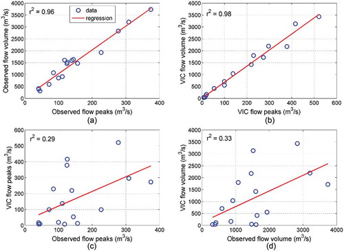
As shown in Figure 6(a) and (b), the streamflow peak and streamflow volume are strongly correlated with one another in both the observed data and the model-simulated data. However, due to uncertainties in snow modeling due to a constant parameter set for all spatial and temporal model grids for each event, the correlations between observed and simulated flow peaks and between observed and simulated flow volumes are not as strong (Fig. 6(c) and (d)). It is important to note that the magnitude of calibration RMSE had no effect on data-based fidelity, as this fidelity was determined based on observed data. However, it is recognized that the calibration error could affect the model-based fidelity, but the assessment of the effects of the calibration accuracy on model-based fidelity was beyond the scope of this study.

Figure 6. Comparisons between observed data and data simulated by VIC: (a) observed flow peaks and observed flow volumes; (b) simulated flow peaks and simulated flow volumes; (c) observed and simulated flow peaks; and (d) observed and simulated flow volumes.

Results

Categorical skill scores

To determine the data-based and model-based hydrologic fidelity of snow gages in this study, four-category contingency tables were calculated with Barnston, LEPS, and GSS for snow depth vs flood peaks, and for snow depth vs flood volumes. The contingency table for snow depth vs flood volumes was nearly identical to that of snow depth vs flow peaks, and it was deemed sufficient to show only one of the two. Table 4 shows the contingency tables for snow depth vs flow peaks. The categories are based on ranked datasets, which are then divided into four approximately equal groups using the three quartiles. The numbers on the diagonal indicate that a flood peak and snow depth for a flood event fall into the same quartile. The first and last columns in Table 4 show the data-based and VIC model-based hydrologic fidelity calculations, respectively. The other two columns compare model flow with observed snow depth, and model snow depth with observed flow. The model–model and data–data comparisons are given in the first and fourth columns in Table 4, respectively. The other two comparisons (model–data and data–model) are shown in the second and third columns, respectively. Although the first and fourth columns directly calculate the data-based and the model-based hydrologic fidelity, the only purpose of the second and third columns is to provide an arbitrary reference level for comparison.

Table 4. Four-by-four contingency tables for snow depth vs flow peaks.

Station	Obs. flow peak vs Obs. snow depth	VIC flow peak vs Obs. snow depth	Obs. flow peak vs VIC snow depth	VIC flow peak vs VIC snow depth
Darlington
Dodgeville
Freeport
Martintown
Monroe

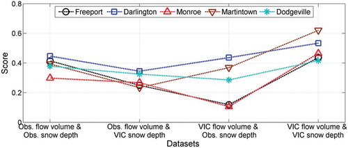
The average variations between the three skill scores at the five sites and for the four different comparisons for snow-flow volume relationships are practically identical to those of snow–flow peak relationships. Figure 7 shows results for snow–flow volume relationships, averaged over the three skill scores for each station. The highest score, and therefore the highest hydrologic fidelity for both data-based and model-based comparisons, is at Darlington, followed by Martintown, indicating that these two stations are more valuable for hydrologicanalyses than the others. The Darlington gage was also found to be one of the most reliable in the region based on quality assessment performed at the MRCC, yet the Martintown gage was not deemed reliable (Leslie Stoecker, MRCC, personal communication). This demonstrates that the rankings based on standard snow gage evaluations do not always match the rankings based on hydrologic fidelity.

Figure 7. Average over the three skill score methods presented for each gaging station for observed and VIC data between snow depths and flow volumes.

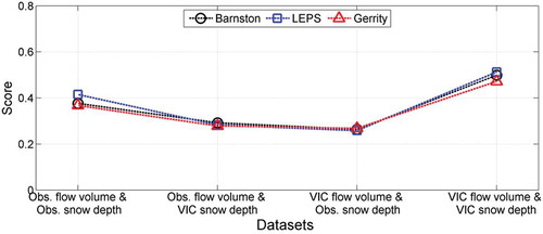
Furthermore, the snow–flow volume relationships were averaged over the five sites to show the performance of each skill score method; these data are presented in Figure 8. Figures 7 and 8 together indicate that the results of the three skill score methods are very consistent, with differences that are much smaller than those between the different sites.

Figure 8. Average over the five stations presented for each skill score method for observed and VIC data between snow depths and flow volumes.

A summary of all the results is given in Table 5, which presents the results for the three methods, the two datasets, and the five gaging sites, illustrating the correspondence between snow depth and flow volume. The correspondence tables for snow depth and flow peaks are not shown here as they are almost identical to those presented in Table 5. It should also be noted that the three skill scores exhibited very similar performance. Further analysis to evaluate these scores indicated that the correlation coefficient between the results of LEPS and Gerrity was the highest (0.97), and other correlations (Barnston–LEPS and Barnston–Gerrity) were lower (0.94). The mean score based on all three methods is 0.35–0.37 for Barnston, and all three standard deviations are equal to 0.13.

Table 5. Skill scores showing the categorical correspondence between snow depth and flow volume for observed and model-generated data at five gaging stations. Bold numbers denote the highest and second highest scores.

Comparison	Obs. flow volume & Obs. snow depth			Obs. flow volume & VIC snow depth			VIC flow volume & Obs. snow depth			VIC flow volume & VIC snow depth
Station	Barnston	LEPS	Gerrity	Barnston	LEPS	Gerrity	Barnston	LEPS	Gerrity	Barnston	LEPS	Gerrity
Freeport	0.424	0.434	0.386	0.235	0.271	0.242	0.141	0.118	0.098	0.424	0.461	0.425
Darlington	0.424	0.479	0.438	0.377	0.325	0.333	0.424	0.421	0.464	0.565	0.521	0.516
Monroe	0.282	0.318	0.294	0.282	0.252	0.268	0.094	0.112	0.111	0.471	0.500	0.425
Martintown	0.329	0.465	0.386	0.235	0.225	0.242	0.329	0.366	0.412	0.612	0.641	0.608
Dodgeville	0.424	0.379	0.333	0.329	0.339	0.307	0.329	0.274	0.255	0.424	0.439	0.386

Overall, Darlington was the most consistent station, showing the highest data-based fidelity, in the form of top scores for each skill score for the observed data. Considering the model-based fidelity, Martintown is the highest for all methods, followed by Darlington. These scores demonstrate that the gage at Darlington had the highest overall fidelity, having both data- and model-based fidelities among the highest across all three methods. The high model-based skill scores for Martintown suggest that this station could be important because of its location within a large central part of the watershed containing the snowpack that is critical to large late-winter floods. It can also be speculated that the somewhat lower data-based hydrologic fidelity at Martintown may have been a result of gage siting issues, which may need to be addressed by additional analysis, potentially resulting in a change in the gage location. Thus, analyses of hydrologic fidelity have the potential to detect strengths and weaknesses of in situ gages, and they could be used as an additional tool in gage network evaluation.

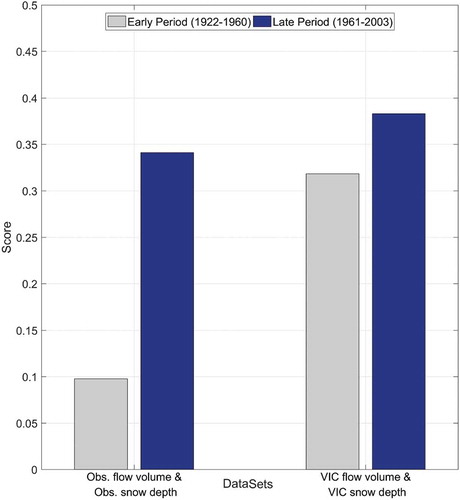
To investigate the temporal changes in hydrologic fidelity, further analysis was carried out, focusing on the Darlington gaging station, which has the highest fidelity in addition to the longest monitoring record. The dataset of 17 floods from this station was divided into two periods: The early period, 1922–1960, which includes the first eight floods; and the late period, 1961–2003, which includes the remaining nine floods. The results show a dramatic 250% improvement in the data-based fidelity, and a 20% improvement in the model-based fidelity shown in Figure 9. This temporal increase in data-based fidelity matches the increase in the accuracy of snow depth measurements, as the recent snow observations in this region are considered more accurate than the early ones. This result supports the assumption of Guan et al. (2013) that more accurate snow data will generally have a higher correlation with river flows, and thus produce a higher hydrologic fidelity. Consequently, changes in hydrologic fidelity could be used as a tool to detect changes in the accuracy of snow depth measurements or heterogeneities in snow depth datasets.

Figure 9. Data-based and model-based averages of the three skill scores between snow depths and flow volumes for early and late periods at Darlington gaging station.

Leave-one-out cross-validation analysis

To determine how much single events affect fidelity we applied the leave-one-out cross-validation (LOOCV) method. The LOOCV method generally uses a single observation from the original dataset and the remaining data as the training data. The LOOCV technique is repeated such that each observation in the sample is used once as the validation data. This approach is the same as the K-fold cross-validation, with K being equal to the number of observations in the original data (McLachlan et al. 2004, Chen and Liu 2012). In this application the Barnston, LEPS, and Gerrity skill scores were calculated based on all 16 years of data except the one (testing year dataset). As can be seen in Figures 10–12, the skill scores for all 17 datasets, marked as circles, ranged between 25th and 75th percentiles of skill scores, with some exceptions, such as VIC flow peak & VIC snow depth data and VIC flow volume & VIC snow depth data at Martintown. Consequently, it can be concluded that the effect of each single event on fidelity is generally minor, but substantial in several instances, which could be explained partly by the relatively small sample size of 17 events. Future studies with larger samples would be useful in determining the effects of sample size on LOOCV analysis results.

Figure 10. LOOCV box plots of Barnston skill scores depending on stations: (a) Freeport; (b) Darlington; (c) Monroe; (d) Martintown; and (e) Dodgeville. Note that black circles are Barnston skill score results for all 17 year datasets.

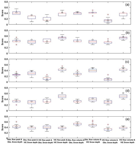
Figure 11. LOOCV box plots of Gerrity skill scores depending on stations: (a) Freeport; (b) Darlington; (c) Monroe; (d) Martintown; and (e) Dodgeville. Note that black circles are Barnston skill score results for all 17 year datasets.

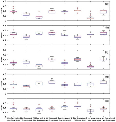
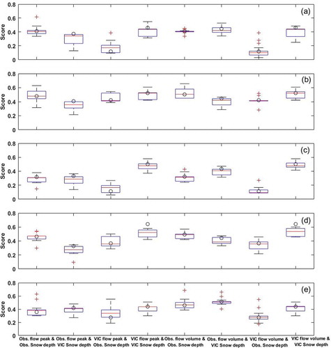
Figure 12. LOOCV box plots of LEPS skill scores depending on stations: (a) Freeport; (b) Darlington; (c) Monroe; (d) Martintown; and (e) Dodgeville. Note that black circles are Barnston skill score results for all 17 year datasets.

Discussion

The quality assessment of snow depth data and the design of snow monitoring networks have been addressed by many researchers (e.g. Molotch and Bales 2005, Mishra and Coulibaly 2009, Gleason et al. 2017). Snow depth is a critical hydrological variable in northern latitudes and requires monitoring networks that will provide the maximum information based on observed data (Mishra and Coulibaly 2009). Guan et al. (2013) assessed SWE monitoring data accuracy through a correlation between the average areal SWE and river flows. Similarly to Guan et al., for each snowmelt-generated hydrograph, we defined data-based hydrologic fidelity as a correspondence between snow depth at each snow depth monitoring site and snowmelt-generated river flows. We also found that the newer, more accurate snow depth data have higher fidelity, which was consistent with the assumption used in Guan et al. (2013) that SWE data with a high correlation (in this case higher categorical correspondence) with river flows are more accurate than those with a low correlation.

Our study also defines model-based fidelity as the correspondence between model-simulated snow depths and hydrograph peaks/volumes. Centrally located snow gages representing larger areas of the watershed that receive higher snowfall are more likely to have higher model-based fidelity than gages located on the watershed edges, representing smaller areas and receiving lesser snowfall. Such snow gages are deemed more representative in snowmelt–runoff modeling. Given that different hydrologic models would generally produce different model-based fidelities, it would be necessary to test this fidelity using a range of approaches, potentially including statistical, data-mining, and complex conceptual models.

Although likely interpretations were offered for the results in this study, it should be recognized that there are numerous data and model uncertainties, including the small sample size of 17 events, data observation errors, lack of observed snow density, model selection, and model calibration/parameterization. Particularly for data observation errors such as snow depth and flow, the new records are generally regarded as more accurate for various reasons, such as digitalization errors of old data (Kunkel et al. 2009), improved procedures for measuring snow, and better training of NWS (US National Weather Service) cooperative observers over time (Jim Angel, Illinois State Climatologist, personal communication), or the ability to send observed data via WxCoder, the web-based data entry system of the Coop Program (Ed Hopkins, Assistant Wisconsin State Climatologist, personal communication).

To reduce these uncertainties, the framework for hydrologic fidelity could be extended to include additional variables, such as the characteristics of the temperature–time series surrounding flood events. Sharp and significant episodes of temperature increase are more likely to produce short-duration snowmelt, and such short and intense events generally result in lower infiltration because the soils remain largely frozen. Short-term temperature increases provide less time for soil to thaw and less time for sublimation and evaporation, which in turn, due to the smaller hydrologic losses, may generate a larger surface runoff. In contrast, minor but persistent temperatures above freezing are more likely to generate a slower and longer hydrologic response. This could increase the likelihood of soil thaw, infiltration, sublimation, and evaporation, thereby reducing the surface runoff and resulting in lower flood volumes and peaks. Including the “flashiness” of the temperature changes could potentially fine-tune the hydrologic fidelity, but a larger sample size than that available in this study would be required. Moreover, it would be difficult to provide a practical definition of flashiness as most events have multiple temperature increase episodes during each snowmelt event. The addition of air humidity, wind speed, or SWE data would be useful in fine-tuning the hydrologic fidelity once these datasets become available. Applications of this methodology to other snowmelt-driven watersheds will determine if and to what degree the concept of hydrologic fidelity can be transferred to other watersheds in similar or different geographical locations. Once validated for different regions, the hydrologic fidelity of snow gages, presented in this study, along with other measures such as the precipitation fidelity (Mobley et al. 2012), will have potential application in evaluating or modifying existing climate monitoring networks.

Conclusions

This study presents the formulation of hydrologic fidelity of snow depth as a categorical skill score between snow depth and corresponding flood characteristics, namely flood peaks and volumes. The hydrologic fidelity is illustrated using the 17 largest snowmelt-dominated runoff events in the Pecatonica River in Wisconsin and Illinois, USA. Although the results based on one case-study cannot be generalized, the study results offer some initial indications. Higher hydrologic fidelities indicate greater benefits of snow depth gages in hydrologic research and applications, such as hydroclimatic studies, trend analyses, flood simulation and forecasting, and thus higher overall value of those measurements. Snow gages with low fidelity have the lowest value for hydrologic studies and potentially could be moved to different locations, or even discontinued should it become necessary to reduce the gage network. Conversely, snow gages with a high fidelity should be continued.

The data-based hydrologic fidelity of snow depth observations in the Pecatonica River was calculated with a four-category matrix, using three different categorical skill scores: the Barnston, the LEPS, and the GSS. The results produce very consistent rankings across all methods for the five gages in the watershed, indicating the stations with the highest fidelity, and those with the lowest. In addition, an analysis indicates a higher fidelity for the snow depth data with higher measurement accuracy, as suggested in previous research. The same framework was also applied to calculate the model-based hydrologic fidelity using the VIC model-generated snow depth and flow data, for which we provided the argument that the stations with the highest model-based fidelity have the greatest potential to simulate the snowmelt–runoff processes accurately. In the Pecatonica River watershed, Darlington and Martintown gages exhibit high rankings for both data- and model-based fidelity, unlike Monroe, which has low rankings for both fidelities.

Although the concept of hydrologic fidelity of snow gages as an additional tool to assess snow monitoring sites and networks needs to be validated through its applications to different regions, the findings of this study provide an initial indication that this concept could be very beneficial if used in addition to the standard quality control procedures for snow depth observation data. Ultimately, these results can be used to support efforts to optimize climate monitoring networks.

Acknowledgements

The authors would like to acknowledge the contribution of Tom Over (USGS), Beth Hall, Michael Machesky, and Lisa Sheppard (ISWS), who provided useful review comments. Dr Jim Angel, Illinois State Climatologist, and Dr Edward J. Hopkins, Assistant Wisconsin State Climatologist, helped with information on snow data monitoring, history of the gages, and quality of the observed data.

Disclosure statement

No potential conflict of interest was reported by the authors.

Additional information

Funding

This research, supported by Illinois State Water Survey (ISWS) and Konkuk University in 2014, represents an extension of a project funded by the Federal Emergency Management Agency, under Award [EMC=2009-CA-7007].

References

- Anderson, E. 1973. National weather service river forecast system-snow accumulation and ablation model, NOAA technical memorandum. NWS Hydro-17. Silver Spring, MD: US National Weather Service.
- Anderson, E.A., 1976. A point of energy and mass balance model of snow cover. Silver Spring, MD: National Weather Service, NOAA Technical Report, 19.
- Andreadis, K.M., Storck, P., and Lettenmaier, D.P., 2009. Modeling snow accumulation and ablation processes in forested environments. Water Resources Research, 45 (5). doi:10.1029/2008WR007042
- Barnston, A.G., 1992. Correspondence among the correlation, RMSE, and Heidke forecast verification measures: refinement of the Heidke score. Weather and Forecasting, 7 (4), 699–709. doi:10.1175/1520-0434(1992)007<0699:CATCRA>2.0.CO;2
- Baxter, M.A., Graves, C.E., and Moore, J.T., 2005. A climatology of snow-to-liquid ratio for the contiguous United States. Weather Forecasting, 20, 729–744. doi:10.1175/WAF856.1
- Benedetti, A., et al., 2005. Verification of TMI-adjusted rainfall analyses of tropical cyclones at ECMWF using TRMM precipitation radar. Journal of Applied Meteorology, 44 (11), 1677–1690. doi:10.1175/JAM2300.1
- Bernal, S. and Sabater, F., 2008. The role of lithology, catchment size and the alluvial zone on the hydrogeochemistry of two intermittent Mediterranean streams. Hydrological Processes, 22 (10), 1407–1418. doi:10.1002/(ISSN)1099-1085
- Bowling, L.C., Pomeroy, J.W., and Lettenmaier, D.P., 2004. Parameterization of blowing-snow sublimation in a macroscale hydrology model. Journal of Hydrometeorology, 5, 745–762. doi:10.1175/1525-7541(2004)005<0745:POBSIA>2.0.CO;2
- Chen, F.-W. and Liu, C.-W., 2012. Estimation of the spatial rainfall distribution using inverse distance weighting (IDW) in the middle of Taiwan. Paddy and Water Environment, 10 (3), 209–222. doi:10.1007/s10333-012-0319-1
- Cherkauer, K.A., Bowling, L.C., and Lettenmaier, D.P., 2003. Variable infiltration capacity cold land process model updates. Global and Planetary Change, 38 (1), 151–159. doi:10.1016/S0921-8181(03)00025-0
- Cherkauer, K.A. and Lettenmaier, D.P., 1999. Hydrologic effects of frozen soils in the upper Mississippi River basin. Journal of Geophysical Research-Atmospheres, 104 (D16), 19599–19610. doi:10.1029/1999JD900337
- Cherkauer, K.A. and Lettenmaier, D.P., 2003. Simulation of spatial variability in snow and frozen soil. Journal of Geophysical Research-Atmospheres, 108 (D22), 8858. doi:10.1029/2003JD003575
- Dziubanski, D.J. and Franz, K.J., 2016. Assimilation of AMSR-E snow water equivalent data in a spatially-lumped snow model. Journal of Hydrology, 540, 26–39. doi:10.1016/j.jhydrol.2016.05.046
- Eder, B., et al., 2006. An operational evaluation of the Eta-CMAQ air quality forecast model. Atmospheric Environment, 40, 4894–4905. doi:10.1016/j.atmosenv.2005.12.062
- Freeze, R.A. and Harlan, R.L., 1969. Blueprint for a physically-based digitally simulated hydrologic response model. Journal of Hydrology, 9, 237–239. doi:10.1016/0022-1694(69)90020-1
- Gandin, L.S. and Murphy, A.H., 1992. Equitable skill scores for categorical forecasts. Monthly Weather Review, 120 (2), 361–370. doi:10.1175/1520-0493(1992)120<0361:ESSFCF>2.0.CO;2
- Gebert, W.A. and Krug, W.R., 1996. Streamflow trends in Wisconsin’s driftless area. Water Resources Bulletin, 32 (4), 733–744. doi:10.1111/j.1752-1688.1996.tb03470.x
- Gerrity, J.P., 1992. A note on Gandin and Murphy’s equitable skill score. Monthly Weather Review, 120 (11), 2709–2712. doi:10.1175/1520-0493(1992)120<2709:ANOGAM>2.0.CO;2
- Gleason, K.E., Nolin, A.W., and Roth, T.R., 2017. Developing a representative snow-monitoring network in a forested mountain watershed. Hydrology and Earth System Sciences, 21 (2), 1137–1147. doi:10.5194/hess-21-1137-2017
- Guan, B., et al., 2013. Snow water equivalent in the Sierra Nevada: blending snow sensor observations with snowmelt model simulations. Water Resources Research, 49, 5029–5046. doi:10.1002/wrcr.20387
- Haklander, A.J. and Van Delden, A., 2003. Thunderstorm predictors and their forecast skill for The Netherlands. Atmospheric Research, 67 (8), 273–299. doi:10.1016/S0169-8095(03)00056-5
- Harr, R.D., 1986. Effects of clearcutting on rain-on-snow runoff in western Oregon: A new look at old studies. Water Resources Research, 22 (7), 1095–1100. doi:10.1029/WR022i007p01095
- Holopainen, M., et al., 2010. Comparing accuracy of airborne laser scanning and TerraSAR-X radar images in the estimation of plot-level forest variables. Remote Sensing, 2 (2), 432. doi:10.3390/rs2020432
- IDNR (Illinois Department of Natural Resources), 1998. Sugar-pecatonica area assessment, volume 2 water resources. Champaign, IL: Office of Scientific Research and Analysis, Illinois State Water Survey.
- Jasper, K. and Kaufmann, P., 2003. Coupled runoff simulations as validation tools for atmospheric models at the regional scale. Quarterly Journal of the Royal Meteorological Society, 129 (588), 673–692. doi:10.1256/qj.02.26
- Jonas, T., Marty, C., and Magnusson, J., 2009. Estimating the snow water equivalent from snow depth measurements in the Swiss Alps. Journal of Hydrology, 378, 161–167. doi:10.1016/j.jhydrol.2009.09.021
- Jörg-Hess, S., et al., 2014. Homogenisation of a gridded snow water equivalent climatology for alpine terrain: methodology and applications. The Cryosphere, 8 ( 10.5194/tc-8-471-2014), 471–485. doi:10.5194/tc-8-471-2014
- Juckem, P.F., et al., 2008. Effects of climate and land management change on streamflow in the driftless area of Wisconsin. Journal of Hydrology, 355 (1–4), 123–130. doi:10.1016/j.jhydrol.2008.03.010
- Kirnbauer, R., Blöschl, G., and Gutknecht, D., 1994. Entering the era of distributed snow models. Nordic Hydrology, 25 (1–2), 1–24.
- Kochendorfer, J.P. and Hubbart, J.A., 2010. The roles of precipitation increases and rural land-use changes in streamflow trends in the Upper Mississippi River Basin. Earth Interact, 14, 1–12
- Kunkel, K.E., et al., 2009. Trends in 20th century US snowfall using a quality-controlled dataset. Journal of Atmospheric and Oceanic Technology, 26, 33–44. doi:10.1175/2008JTECHA1138.1
- Liang, X., et al., 1994. A simple hydrologically based model of land surface water and energy fluxes for general circulation models. Journal of Geophysical Research: Atmospheres (1984–2012), 99 (D7), 14415–14428. doi:10.1029/94JD00483
- Liang, X., Lettenmaier, D.P., and Wood, E.F., 1996. One-dimensional statistical dynamic representation of subgrid spatial variability of precipitation in the two-layer variable infiltration capacity model. Journal of Geophysical Research, 101 (D16), 21403–21422. doi:10.1029/96JD01448
- Livezey, R.E., 2012. Deterministic forecasts of multi-category events. In: I.T. Jolliffe and D. B. Stephenson, eds. Forecast verification: a practitioner’s guide in atmospheric science. 2nd ed. West Sussex: Willey-Blackwell, 61–75.
- Lohmann, D., et al., 1998. Regional scale hydrology: I. Formulation of the VIC-2L model coupled to a routing model. Hydrological Sciences Journal, 43 (1), 131–141. doi:10.1080/02626669809492107
- Lohmann, D., Nolte‐Holube, R., and Raschke, E., 1996. A large‐scale horizontal routing model to be coupled to land surface parametrization schemes. Tellus A, 48 (5), 708–721. doi:10.3402/tellusa.v48i5.12200
- Marks, D., et al., 1998. The sensitivity of snowmelt processes to climate conditions and forest cover during rain-on-snow: A case study of the 1996 Pacific Northwest flood. Hydrological Processes, 12 (10), 1569–1587. doi:10.1002/(SICI)1099-1085(199808/09)12:10/11<1569::AID-HYP682>3.0.CO;2-L
- Markus, M., et al., 2010. Prediction of weekly nitrate-N fluctuations in a small agricultural watershed in Illinois. Journal of Hydroinformatics, 12 (1), 251–261. doi:10.2166/hydro.2010.064
- Markus, M., et al., 2013. Episodic change analysis of the annual flood peak time series for a flood insurance study. Journal of Hydrologic Engineering, 18 (1), 85–91. doi:10.1061/(ASCE)HE.1943-5584.0000604
- Maurer, E.P., et al., 2002. A long-term hydrologically based dataset of land surface fluxes and states for the conterminous United States. Journal of Climate, 15 (22), 3237–3251. doi:10.1175/1520-0442(2002)015<3237:ALTHBD>2.0.CO;2
- McCabe, G.J., Hay, L.E., and Clark, M.P., 2007. Rain-on-snow events in the western United States. Bulletin of the American Meteorological Society, 88 (3), 319–328. doi:10.1175/BAMS-88-3-319
- McLachlan, G.J., Ambroise, K.-A., and Do, C., 2004. Analyzing microarray gene expression data. New York: Wiley.
- Mishra, A.K. and Coulibaly, P., 2009. Developments in hydrometric network design: A review. Reviews of Geophysics, 47, 1–24. doi:10.1029/2007RG000243
- Mishra, V. and Cherkauer, K.A., 2011. Influence of cold season climate variability on lakes and wetlands in the Great Lakes region. Journal of Geophysical Research-Atmosphere, 116, D12111. doi:10.1029/2010JD015063
- Mishra, V., Cherkauer, K.A., and Shukla, S., 2010. Assessment of drought due to historic climate variability and projected future climate change in the Midwestern United States. Journal of Hydrometeorology, 11 (1), 46–68. doi:10.1175/2009JHM1156.1
- Mobley, J.T., Culver, T.B., and Burgholzer, R.W., 2012. Understanding precipitation fidelity in hydrological modeling. Journal of Hydrologic Engineering, 17 (12), 1315–1324. doi:10.1061/(ASCE)HE.1943-5584.0000588
- Molotch, N.P. and Bales, R.C., 2005. Scaling snow observations from the point to the grid element: implications for observation network design. Water Resources Research, 41, W11421. doi:10.1029/2005WR004229
- Myneni, R.B., Nemani, R.R., and Running, S.W., 1997. Estimation of global leaf area index and absorbed par using radiative transfer models. IEEE Transactions of Geoscience and Remote Sensing, 35 (6), 1380–1393. doi:10.1109/36.649788
- Park, D. and Markus, M., 2014. Analysis of changing hydrologic flood regime using the variable infiltration capacity model. Journal of Hydrology, 515, 267–280. doi:10.1016/j.jhydrol.2014.05.004
- Potter, K.W., 1991. Hydrological impacts of changing land management practices in a moderate-sized agricultural catchment. Water Resources Research, 27, 845–855. doi:10.1029/91WR00076
- Potts, J.M., et al., 1996. Revised “LEPS” scores for assessing climate model simulations and long-range forecasts. Journal of Climate, 9, 34–53. doi:10.1175/1520-0442(1996)009<0034:RSFACM>2.0.CO;2
- Rodwell, M. J., et al., 2010. A new equitable score suitable for verifying precipitation in numerical weather prediction. Quarterly Journal of the Royal Meteorological Society, 136 (650), 1344–1363.
- Roebber, P.J., et al., 2002. Improving snowfall forecasting by diagnosing snow density. Weather Forecast, 18 (2), 264–287. doi:10.1175/1520-0434(2003)018<0264:ISFBDS>2.0.CO;2
- Sinha, T. and Cherkauer, K.A., 2010. Impacts of future climate change on soil frost in the Midwestern United States. Journal of Geophysical Research – Atmospheres, 115, 1–16.
- Sinha, T., Cherkauer, K.A., and Mishra, V., 2010. Impacts of historic climate variability on seasonal soil frost in the Midwestern United States. Journal of Hydrometeorology, 11 (2), 229–252. doi:10.1175/2009JHM1141.1
- Tan, A., Adam, J.C., and Lettenmaier, D.P., 2011. Change in spring snowmelt timing in Eurasian Arctic rivers. Journal of Geophysical Research – Atmospheres, 116, 1–12
- Tarboton, D.G., Chowdhury, T.G., and Jackson, T.H., 1994. A spatially distributed energy balance snowmelt model. Proceedings of the Biogeochemistry of Seasonally Snow Covered Catchments, 144–155.
- Varhola, A., et al., 2010. A new low-cost, stand-alone sensor system for snow monitoring. Journal of Atmospheric and Oceanic Technology, 27, 1973–1978. doi:10.1175/2010JTECHA1508.1
- Ward, M.N. and Folland, C.K., 1991. Prediction of seasonal rainfall in the north Nordeste of Brazil using eigenvectors of sea‐surface temperature. International Journal of Climatology, 11 (7), 711–743. doi:10.1002/joc.3370110703
- Wigmosta, M.S., Vail, L.W., and Lettenmaier, D.P., 1994. A distributed hydrology-vegetation model for complex terrain. Water Resources Research, 30 (6), 1665–1679. doi:10.1029/94WR00436
- Yossef, N.C., et al., 2012. Assessment of the potential forecasting skill of a global hydrological model in reproducing the occurrence of monthly flow extremes. Hydrology and Earth System Sciences, 16 (11), 4233–4246. doi:10.5194/hess-16-4233-2012
- Zappa, M., 2008. Objective quantitative spatial verification of distributed snow cover simulations—an experiment for the whole of Switzerland. Hydrological Sciences Journal, 53 (1), 179–191. doi:10.1623/hysj.53.1.179