Definitions of climatological and discharge days: do they matter in hydrological modelling?

ABSTRACT

The performance of hydrological models is affected by uncertainty related to observed climatological and discharge data. Although the latter has been widely investigated, the effects on hydrological models from different starting times of the day have received little interest. In this study, observational data from one tropical basin were used to investigate the effects on a typical bucket-type hydrological model, the HBV, when the definitions of the climatological and discharge days are changed. An optimization procedure based on a genetic algorithm was used to assess the effects on model performance. Nash-Sutcliffe efficiencies varied considerably between day definitions, with the largest dependence on the climatological-day definition. The variation was likely caused by how storm water was assigned to one or two daily rainfall values depending on the definition of the climatological day. Hydrological models are unlikely to predict high flows accurately if rainfall intensities are reduced because of the day definition.

EDITOR:

• A. Castellarin

ASSOCIATE EDITOR:

• A. Viglione

KEYWORDS:

• climatological day
• discharge day
• rainfall–runoff model
• daily resolution
• regionalization
• floods

1 Introduction

The accuracy and performance of hydrological models are affected by quantity and quality of forcing and calibration data (Gan et al. 1997), spatial and temporal variability of precipitation (Xu et al. 2013, Girons Lopez and Seibert 2016), and temporal resolution of data (Littlewood and Croke 2008, Kavetski et al. 2011, Reynolds et al. 2017, Jie et al. 2018). Climatological and discharge time series are often only available at a daily resolution whereas many rainfall–runoff models are applied at a temporal resolution equal to or lower than daily (Melsen et al. 2016).

The temporal resolution at which model outputs are analysed is in most cases defined by the temporal sampling at which observations are stored or made available, often at a daily or monthly resolution (Kavetski et al. 2011). There is a vast literature on how temporal resolution affects model results, but we are unaware of any hydrological studies concerning the datum of the daily time step, i.e. the starting time of the day. A variety of factors influence this datum, in the following named definition of the day, and the use of inconsistent starting times could potentially create problems. When data are averaged over many days for monthly or annual applications such inconsistencies may not be significant (Chiew and McMahon 1994). It could, however, be expected that they will affect parameter estimates and runoff predictions at a daily resolution, which may have implications for regionalization and flood forecasting, and potentially lead to poor information for water resources planning.

A few climatological studies have raised the issue of inconsistent definitions of the day. Vincent et al. (2009) reported that different definitions of the climatological day cause a bias in the annual and seasonal means of daily minimum temperature across Canada, whereas the means of daily maximum temperature are unaffected. Hutchinson et al. (2009) presented spatial models of daily maximum–minimum temperature and precipitation in Canada for 1961–2003 and reported larger than expected residuals between observed and estimated values, assumedly related to inconsistent definition of the climatological day of the interpolation data. The temporal incommensurability problem is sometimes touched upon in hydrology, e.g. when Westerberg et al. (2014) reported a daily discharge correction of 17% because observed data were not registered continuously.

Manual observations of daily climatological variables (such as precipitation and temperature) are commonly done once or twice per 24 hours. Rainfall is measured daily at ordinary raingauge stations at fixed hours between 07:00 and 09:00 local standard time (LST), and the total amount of rainfall is assigned to the previous calendar day (WMO 2011). From a practical point of view, observation times are often adapted to the observers’ working hours, with one morning observation and an optional second in the afternoon. Daily discharge is commonly computed from midnight to midnight from instantaneous discharge values, processed from recorded gauge heights (WMO 2010). In the past, daily discharge was computed from daily average gauge height or from gauge heights averaged over parts of a day (WMO 2010). Daily rainfall and daily discharge may thus refer to different 24-h intervals.

Operational flood-forecasting models are typically fed with 6-h rainfall forecasts derived from numerical weather-prediction (NWP) models within ensemble-prediction systems (EPS) (Wetterhall et al. 2011). Rainfall forecasts from NWP-EPS are released at 6-h intervals starting at 12:00 coordinated universal time (UTC). Model forecasts should be used with parameters calibrated at the 6-h resolution based on UTC and not on local time. Given that long time series of rainfall and discharge at sub-daily temporal resolutions are rare, rainfall–runoff models are usually calibrated at the daily resolution. These parameter values are then used with the 6-h rainfall for flood forecasting. This approach has been criticized because of inaccuracies of the daily parameters (Littlewood and Croke 2008) or because of poor model performance (Bastola and Murphy 2013), which may partly be caused by the definitions of the climatological and discharge days.

This study aimed at assessing how different definitions of the climatological and discharge days affected a rainfall–runoff model. We used a basin in Panama and a typical bucket-type hydrological model. Rainfall–runoff data were available at a high temporal resolution, which allowed us to change the definitions of the climatological and discharge days in different 24-h intervals. Our questions were: (1) Do the definitions of the climatological and discharge days impact the performance and accuracy of our model? And (2) If they do, which definition between climatological and discharge days affects the model the most?

2 Material and methods

2.1 Study site

The tropical Boqueron River basin drains to the Panama Canal. The 91 km² basin is predominantly covered by forests, and its elevation ranges from 100 to 980 m a.s.l. (USGS 2016). Lag time is 1−3 h. Rainfall in the region depends on: (1) the annual movement of the inter-tropical convergence zone; (2) the presence of northeast trade winds; (3) the mountainous terrain (Georgakakos et al. 1999); and (4) the ENSO phenomenon (Ropelewski and Halpert 1987). Climate is characterized by a dry (January−April) and a rainy season (May−December). Rainfall is generally convective and orographic, and occurs mostly in the form of heavy downpours resulting from thunderstorms. The 1997–2011 mean annual rainfall in the basin is 3800 mm year⁻¹ and runoff 2728 mm year⁻¹.

We estimated areal precipitation by Thiessen polygons from four stations of hourly rainfall data, available within and close to the basin for 1997−2011. Stage at the Peluca station (basin outlet) was recorded continuously in a nonstationary river cross section using a float inside a stilling well and stored every 15 minutes. Stage–discharge ratings at this station are made at least once a month and rating-curve updates are made in case of change. Discharge (m³ s⁻¹) for 1997−2011 was converted to runoff (mm h⁻¹). Daily pan evaporation for 1985−2010 from the Tocumen station, located 36 km southeast of the basin, was used to estimate long-term daily mean values of potential evaporation. The hydro-meteorological data in this study had previously been quality controlled by Reynolds et al. (2017).

2.2 The HBV model

The HBV model (Bergström 1976, Lindström et al. 1997) is a bucket-type hydrological model that simulates river runoff using precipitation, air temperature and potential evaporation as input data. We used the HBV-light version (v. 4.0.0.17; available at http://www.geo.uzh.ch/en/units/h2k/Services/HBV-Model.html) with its standard model structure set up in a spatially lumped way. Detailed descriptions of the model are given by Bergström (1992), Seibert and Vis (2012) and Reynolds et al. (2017).

The model has been applied successfully in many basins with different climatological conditions, including tropical for design floods (Harlin and Kung 1992, Zeng et al. 2016), flood forecasting (Häggström et al. 1990, Amenu and Killingtveit 2001, Kobold and Brilly 2006), climate change (Chen et al. 2012), for estimation of sediment yield (Liden 1999) and regionalization (Seibert 1999). It was chosen because: (1) it only required precipitation and a long-term estimate of potential evaporation as input, which were available for the study basin; (2) it is representative of many bucket-type hydrological models used for water-resources planning, operational forecasting and research; and (3) simple models like the HBV have been shown to provide as good results as more complex models when hydrograph prediction is the variable of interest (Beven 2001).

2.3 Climatological- and discharge-day definitions

We aggregated 1-h rainfall and runoff data to 12 different sets of daily values. A first daily time series resulted from aggregating the 1-h data for the time interval 00−00, a second for the 02−02 interval, and consecutively every two hours until 22−22. The hour designations refer to LST in Panama (UTC-5 h).

2.4 Numerical experiment

The differential equations in the HBV-light version are solved numerically using the explicit Euler and operator-splitting schemes (adding or subtracting fluxes in a distinct order). These simple methods can be numerically unstable and can return unreliable numerical solutions when used with a daily modelling time step. To avoid numerical artefacts related to the latter, daily runoff was simulated with a 1-h modelling time step, for practical purposes, regardless of the daily input data. Each of the 12 daily rainfall time series was first disaggregated uniformly into 1-h time series to drive the model and generate 1-h runoff. Subsequently, 1-h runoff simulations were aggregated to daily steps based on the 24-h interval for each of the 12 daily runoff time series. This resulted in 144 model set-ups for optimization (i.e. 12 daily rainfall time series, one for each climatological-day definition, for each of the 12 daily runoff time series). Shorter modelling time steps were not considered because a preliminary experiment, in which several numerical solutions were compared, showed that the numerical solution implemented in this study returned solutions similar to those when the implicit Euler method was used with a daily modelling time step, and because it would have made the experiment computationally more demanding. One year (2004) was used to warm up the model which was then calibrated for 1 January 2005–31 December 2011.

2.5 Model calibration

Genetic algorithm optimization is one way to search global optima in conceptual rainfall–runoff models (Kuczera 1997, Seibert 2000). The HBV-light version includes a genetic algorithm (GA) for automatic model calibration. This algorithm generates optimized parameter sets from randomly selected parameter sets by an evolutionary mechanism of selection and recombination (Seibert and Vis 2012). The chance of a generated parameter set to be chosen depends on the value of the objective function, where the parameter set with the best fit gets the highest probability to be chosen. Seibert (2000) describes the GA optimization tool in detail.

Optimized parameter sets were automatically searched for every model set-up using the GA tool based on initial parameter-value ranges taken from the literature (Table 1). We randomly generated an initial population of 50 parameter sets and the number of model runs was set to 5000. We chose the commonly used Nash‐Sutcliffe efficiency (R_eff) as objective function.

Table 1. Parameter ranges used for model calibration.

Parameter	Description	Min−Max	Unit
Soil moisture routine
PFC	Maximum soil-moisture storage	50–1000	mm
PLP	Soil-moisture value above which actual evaporation reaches potential evaporation.	0.0–1.0	-
PBETA	Determines the relative contribution to runoff from rainfall	0.1–5.0	-
Response routine
PPERC	Threshold parameter	2.4–19.2	mm d^−1
PALPHA	Nonlinearity coefficient	0.1–2.0	-
PK1	Storage coefficient 1	0.0024–1.2	d^−1
PK2	Storage coefficient 2	0.0012–0.72	d^−1
Routing routine
PMAXBAS	Length of isosceles triangular weighting function	1.0–6.0	h

3 Results

3.1 Effects of the definitions of the climatological and discharge days on model performance and optimized parameter sets

The definitions of both the climatological and discharge days had a large impact on the maximum model performance (Fig. 1). Model performance varied greatly along both axes and changed gradually, shifting parallel to the main diagonal (Figs. 1 and 2(a)). The main diagonal refers to when both climatological and discharge day definitions were the same. Along the main diagonal, Nash-Sutcliffe efficiencies were high and varied considerably between 0.871 and 0.921, about 0.05 efficiency units. However, the highest efficiencies were found when the 24-h runoff interval lagged the 24-h rainfall interval by 2–4 h. For those cases, the model had sufficient water in storage before the largest runoff peaks had occurred, which facilitated the model to fit the observations (e.g. rainfall/runoff intervals: 22–22/02–02; 02–02/04–04 and 12–12/16–16). Model performance showed a strong decrease for larger lags or when the 24-h rainfall interval lagged the 24-h runoff interval (e.g. rainfall/runoff intervals: 06–06/04–04; 06–06/16–16; 10–10/06–06 and 04–04/20–20). For the latter cases, contrary to those with the highest model performances, the system lacked rainfall to fit the largest runoff peaks, and model performance depended on the amount of rain that had entered the system at the occurrence of those large events.

Figure 1. Two- and three-dimensional views of maximum Nash-Sutcliffe efficiencies (R_eff) achieved by automatic calibration. The black line (main diagonal 00–22) refers to model set-ups with the same day definitions for both climatological and discharge data. The green star represents the best model set-up, whereas the red star represents the worst.

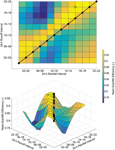
The combination of the 16–16 rainfall and 20–20 runoff intervals returned the highest performance (R_eff = 0.936) whereas the combination of the 06–06 rainfall and 16–16 runoff intervals returned the lowest performance (R_eff = 0.762), an R_eff difference of around 0.17 units. These two combinations are referred to as the best and the worst model set-ups. This difference resulted from an overall agreement between observations and simulations, not just from a few events. An additional experiment, excluding the five largest flows of every daily runoff time series, resulted in an R_eff difference of about 0.19 units. The performance space was almost the same as in Figure 1 but with lower R_eff values (0.06 efficiency units in average).

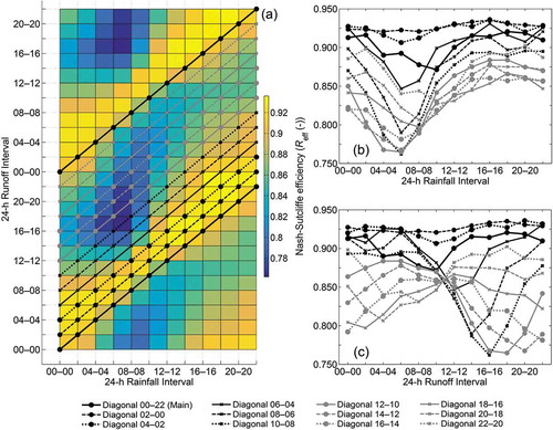
Efficiencies varied considerably along the other diagonals as well (Fig. 2). The R_eff varied moderately between 0.820 and 0.936 for rainfall intervals 12–12, 14–14, 16–16, 18–18, 20–20, 22–22 and 00–00 (Fig. 2(b)), whereas the variability was higher for intervals 02–02, 04–04, 06–06, 08–08 and 10–10. From the latter, the rainfall interval that had the greatest performance variability was 06–06, between 0.762 and 0.923. Model performance varied greatly for most of the 24-h runoff intervals, except for 06–06, 08–08, 10–10 and 12–12 (Fig. 2(c)). If the definition of the climatological day is adequate, then model performance varies less regardless of the definition of the discharge day. The latter was confirmed by using hourly rainfall data as input to simulate daily runoff with different starting times of the day. This eliminated the effects caused by the definition of the climatological day, and as a result, those effects caused by the definition of the discharge day were almost non-existent.

Figure 2. Maximum Nash-Sutcliffe efficiencies (R_eff) of every diagonal: (a) 2-D view of model performance space (same as upper panel of Fig. 1 but replicated vertically). Model performance of every diagonal along the 24-h (b) rainfall–interval axis and (c) runoff–interval axis. In the legend, integer numbers of every R_eff diagonal refer to the 24-h runoff interval at which the diagonal starts and ends in (a) (from left to right).

Model performance for specific 24-h intervals could be explained by exploring the hourly distribution of rainfall and runoff during calibration. The hourly rainfall and runoff distributions were bimodal with two maxima: a small morning peak between 06:00 and 09:00 LST for rain and between 07:00 and 10:00 LST for runoff, and a large afternoon peak between 13:00 and 16:00 LST for rain and between 15:00 and 19:00 LST for runoff. The relative size of the two peaks in every climatological- and discharge-day definition shifted for daily rainfall totals exceeding 100 mm d⁻¹ and for daily runoff totals exceeding 60 mm d⁻¹, such that the largest volumes of both occurred between 07:00 and 10:00 LST for rain and between 10:00 and 12:00 LST for runoff. Since the Nash-Sutcliffe efficiency puts more weight on periods with high flows (Jie et al. 2016), and those were usually not well reproduced when the climatological-day definition split the most extreme rainfall events, it was generally difficult to achieve high model performance. However, model performance varied less for some 24-h runoff intervals because the extreme runoff events were split into two, which made it less problematic to fit the observations even when those runoff intervals were combined with an inadequate 24-h rainfall interval.

The parameter space of the optimized values did not show any clear patterns. However, the optimized parameter values helped to gain understanding of model behaviour in each set-up (e.g. to see how slow or fast rainfall was routed through the model to form total runoff and fit the observations).

3.2 Analysis based on time of occurrence

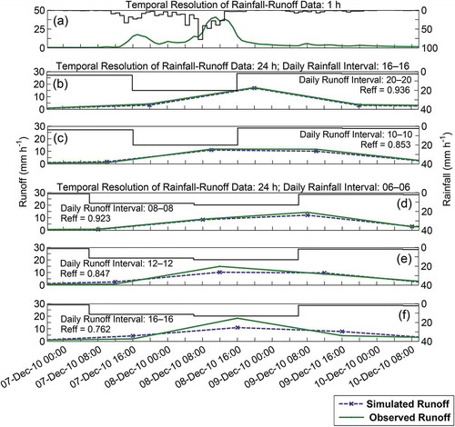
The behaviour of simulations with different day definitions was illustrated by hydrographs from an extreme event (Fig. 3). This event, lasting approximately 24 h, was characterized by moderate rainfall intensities in the beginning and high towards the end, with a peak at 07:00–08:00 LST on 8 December 2010 (Fig. 3(a)). The first daily hydrograph (Fig. 3(b)), from the best model set-up (rainfall/runoff intervals: 16–16/20–20), reproduced the high flow well. For this case, since most of the rain and highest 1-h rainfall intensities were captured within the same 24-h interval, the average value of these intensities resulted in a high daily rainfall value. The 24-h rainfall interval of the second daily hydrograph (Fig. 3(c)) was the same as in the former, but the runoff event was split into two intervals because of the discharge-day definition (10–10). All rainfall had already entered the system before the second discharge peak, but the smooth model routing merged the two high-flow values. The 24-h rainfall interval of the third, fourth and fifth daily hydrographs (Fig. 3(d)–(f)) was 06–06, shown to give the highest model-performance variability in Figure 2(b). This day definition splits the rainfall event into two 24-h intervals and the highest 1-h rainfall intensity was captured in an interval characterized by low or no rainfall. When the two 24-h intervals were averaged to daily, this gave us two moderate rainfall intensities that resulted in both good and bad model fits. The performance differences for this rainfall-day definition were caused by the discharge-day definition in each case. In the third daily hydrograph (Fig. 3(d), rainfall/runoff intervals: 06–06/08–08, close to the main diagonal), almost all rainfall had entered the system before the largest runoff peak and the model was able to route gradually to fit the observations. In the fourth and fifth daily hydrographs (Fig. 3(e)–(f)), the largest runoff peak occurred before all rainfall had entered the system, which the model had problems to reproduce. Simulated runoff in these two cases was similar, but model performance in the latter was worse than in the former because the discharge-day definition in the last one captured almost the entire runoff response in one 24-h interval, which resulted in a larger observed runoff peak and therefore in a worst model fit. The fifth daily hydrograph came from the worst model set-up (rainfall/runoff intervals: 06–06/16–16).

Figure 3. Hydrographs of an extreme rainfall–runoff event: (a) observed 1-h rainfall and runoff data; (b)–(f) daily runoff simulations for model set-ups with different definitions of the climatological and discharge day. Sub-plot (b) corresponds to the best model set-up and (f) to the worst.

4 Discussion

The temporal resolution in hydrological models is normally determined by the temporal resolution at which data are collected (Kavetski et al. 2011). Ideally, the temporal resolution of analysis should be defined by the time scale of the dominant hydrological processes. However, in many regions in the world with small and medium-sized basins, it is a common situation that modelling with data at the temporal resolution needed is not an option and hydrologists have to make use of the best data available. Hydro-meteorological data have increasingly become available at sub-daily resolution (Girons Lopez and Seibert 2016) but daily data are still the most common. These data often come from hydro-meteorological offices with limited information on quality and uncertainties. The definitions of the climatological and discharge days are seldom available or presented when data are used for hydrological modelling. For daily rainfall–runoff modelling, the definition of the climatological and discharge day is likely to affect modelling results if the basin responses occur at time scales finer than daily and should therefore be presented.

This study showed that the definition of the climatological and discharge days had large implications on the HBV model calibration and runoff simulations. Several reasons could explain our results: hydrograph fitting through optimized parameter sets, probability of occurrence of rainfall during the day, duration of rainfall events and discharge responses, as well as timing and correlation between daily rainfall and runoff.

The strong decrease in model performance when the two day definitions differed by more than a few hours or when the 24-h rainfall interval lagged the 24-h runoff interval was expected. Model performance varied by about 0.05 efficiency units when the two day definitions agreed, but more surprising was the finding that it varied gradually when both day definitions were shifted in parallel to the main diagonal. Furthermore, we expected the best model performance to be found when the climatological- and discharge-day definitions coincided. This did not fully turn out to be the case, and the reason could possibly be the inherent nonlinearity of the rainfall–runoff response of the basin or errors in the model structure.

Model performance was more dependent on the definition of the climatological day than on the definition of the discharge day. When a storm overlapped two daily observations because of the climatological-day definition, rainfall intensities were reduced and accurate hydrograph predictions were then only possible if most of the rainfall event (if not all) had entered the hydrological system before the largest discharge peaks. Therefore, we assumed that the main reason for performance differences was the effect of how storm water (1-h observations) was assigned to one or more daily rainfall values. If the climatological day is poorly defined, the way continuous runoff records are assigned to daily runoff values will determine how well a model fits observations. The model chosen smoothed some lags between the rainfall and discharge-day definitions through runoff routing. Other lags caused larger problems because of low rain intensities, in combination with poor timing between daily rainfall and runoff.

Performance in rainfall–runoff models is affected by several sources of uncertainty related to the data and model. Their effects on model performance depend on the basin complexities, calibration period, temporal resolution and modelling purpose. For three basins with different climatological conditions, Pianosi and Wagener (2016) reported that the influence of parameter uncertainty on model performance was larger than that from data uncertainty, but the latter might be more influential in wet conditions and in short time scales. The definitions of the climatological and discharge days are a data-related uncertainty. Given that uncertainty of the data considerably affects the uncertainty of models in calibration, we assume that the definitions of the climatological and discharge days of the data are as important and influential in hydrological modelling as other widely investigated sources of uncertainty. The differences in model performance resulting between the different day definitions were of the same order of magnitude as the differences typically observed when using different periods for calibration (Das et al. 2008, Girons Lopez and Seibert 2016) or different representations of spatial variability (Das et al. 2008). We hypothesise that rainfall–runoff modelling in small and flashy basins, similar to the one used here, located in a region with clear diurnal patterns and with rainfall characterized by storms of high intensity and short duration, will be strongly affected by the day definitions of input and calibration data. The effect is probably less pronounced when rain intensities are low and durations are long, or when heavy rainfall is evenly distributed over the diurnal cycle. We would also expect day definitions to be less significant in large basins where spatial variability is more important than temporal (Beven 2001) because storms only affect part of the basin area (Rosbjerg et al. 2013). The HBV model is similar to many bucket-type models frequently used in practice and research. The results found in this study make us believe that these effects depend more on data than on model and that any hydrological model will likely be affected by this phenomenon, which should be considered for any daily rainfall–runoff model application. This study was motivated by an unexpected result that we found important to publish and it would be desirable to extend it to different basins and different rainfall regimes as well as to additional models with different complexity.

Our work took advantage of the GA optimization tool available in the HBV-light software. The finding that the parameter space of the optimized values did not show any clear pattern was to some extent expected because automatic calibration in hydrological models is an ill-posed problem (Kuczera 1997, Beven 2001). There are several reasons for this: (1) the calibration data may not support the robustness of the optimized parameter set for any algorithm (Beven 2001); (2) the response surface in the parameter space may differ for different algorithms and may have more than one local optimum (i.e. model nonlinearities) (Kuczera 1997); (3) there may be many parameter sets as good as the one found in the optimization procedure (i.e. equifinality) (Beven 2009). Although we do not think that model performance results are very sensitive to the calibration method, it would also be valuable to assess the effects on parameter estimates from different starting times of the day with more elaborated methods in future studies (e.g. the generalized likelihood uncertainty estimation method, GLUE, or the formal Bayesian method).

5 Conclusions

In this study, we explored the effects of the definitions of the climatological and discharge days on a rainfall–runoff model and the results imply that the day definitions may influence regionalization and flood-forecasting applications. The specific conclusions from our analysis are listed below:

1. Nash-Sutcliffe efficiencies varied considerably with the definitions of the climatological and discharge days.

2. As expected, model performance decreased largely when the day definitions for climatology and discharge differed by more than a few hours.

3. Model performance did also vary considerably when the two definitions agreed but for different daily intervals.

4. Model performance was more dependent on the definition of the climatological day than on the definition of the discharge day.

5. Rainfall–runoff models may fail high-flow predictions if rain intensities are reduced by the definition of the climatological day.

This study was limited to one basin, one model, and one calibration method. We call for further studies towards this field to prove the generality of our results.

Acknowledgements

The authors thank the Panama Canal Authority (ACP) who provided the rainfall and discharge data from the Boqueron River basin and the Department of Hydrometeorology at Empresa de Transmisión Eléctrica, S.A. (ETESA) who provided the pan-evaporation data. The authors also thank the three anonymous reviewers for their constructive comments and suggestions for improving the manuscript.

Disclosure statement

No potential conflict of interest was reported by the authors.

Additional information

Funding

This research was carried out within the CNDS research school, supported by the Swedish International Development Cooperation Agency (Sida) through their contract with the International Science Programme (ISP) at Uppsala University (contract number: 54100006).

References

- Amenu, G.G. and Killingtveit, Å. (2001). Real-time inflow forecasting for GilgelGibe reservoir, Ethiopia. In: Hydropower in the New Millennium: Proceedings of the 4th International Conference Hydropower, Bergen, Norway.
- Bastola, S. and Murphy, C., 2013. Sensitivity of the performance of a conceptual rainfall–runoff model to the temporal sampling of calibration data. Hydrology Research, 44 (3), 484–493. doi:10.2166/nh.2012.061
- Bergström, S., 1976. Development and application of a conceptual runoff model for Scandinavian catchments. Norrköping, Sweden: SMHI, Report No. RHO 7.
- Bergström, S., 1992. The HBV model – its structure and applications. Norrköping, Sweden: SMHI Hydrology, RH No. 4.
- Beven, K., 2001. Rainfall–runoff modelling: the primer. Chichester: Wiley.
- Beven, K., 2009. Environmental modelling: an uncertain future? London: Routledge.
- Chen, H., et al., 2012. Impacts of climate change on the Qingjiang Watershed’s runoff change trend in China. Stochastic Environmental Research and Risk Assessment, 26, 847–858. doi:10.1007/s00477-011-0524-2
- Chiew, F. and McMahon, T., 1994. Application of the daily rainfall–runoff model MODHYDROLOG to 28 Australian catchments. Journal of Hydrology, 153 (1–4), 383–416. doi:10.1016/0022-1694(94)90200-3
- Das, T., et al., 2008. Comparison of conceptual model performance using different representations of spatial variability. Journal of Hydrology, 356 (1–2), 106–118. doi:10.1016/j.jhydrol.2008.04.008
- Gan, T.Y., Dlamini, E.M., and Biftu, G.F., 1997. Effects of model complexity and structure, data quality, and objective functions on hydrologic modeling. Journal of Hydrology, 192 (1–4), 81–103. doi:10.1016/S0022-1694(96)03114-9
- Georgakakos, K.P., et al. 1999. Design and tests of an integrated hydrometerorological forecast system for the operational estimation and forecasting of rainfall and streamflow in the mountainous Panama Canal watershed. San Diego, CA: Hydrologic Research Center, HRC Technical Report No. 2.
- Girons Lopez, M. and Seibert, J., 2016. Influence of hydro-meteorological data spatial aggregation on streamflow modelling. Journal of Hydrology, 541, 1212–1220.doi:10.1016/j.jhydrol.2016.08.026
- Häggström, M., et al. 1990. Application of the HBV model for flood forecasting in six Central American rivers. Norrköping, Sweden: SMHI Hydrology, No. 27.
- Harlin, J. and Kung, C.-S., 1992. Parameter uncertainty and simulation of design floods in Sweden. Journal of Hydrology, 137, 209–230. doi:10.1016/0022-1694(92)90057-3
- Hutchinson, M.F., et al., 2009. Development and testing of Canada-wide interpolated spatial models of daily minimum-maximum temperature and precipitation for 1961-2003. Journal of Applied Meteorology and Climatology, 48 (4), 725–741. doi:10.1175/2008JAMC1979.1
- Jie, M.-X., et al., 2016. A comparative study of different objective functions to improve the flood forecasting accuracy. Hydrology Research, 47 (4), 718–735. doi:10.2166/nh.2015.078
- Jie, M.-X., et al. 2018. Transferability of conceptual hydrological models across temporal resolutions: approach and application. Water Resources Management, 32, 1367–1381. doi:10.1007/s11269-017-1874-4
- Kavetski, D., Fenicia, F., and Clark, M.P., 2011. Impact of temporal data resolution on parameter inference and model identification in conceptual hydrological modeling: insights from an experimental catchment. Water Resources Research, 47, W05501. doi:10.1029/2010WR009525
- Kobold, M. and Brilly, M., 2006. The use of HBV model for flash flood forecasting. Natural Hazards and Earth System Science, 6 (3), 407–417. doi:10.5194/nhess-6-407-2006
- Kuczera, G., 1997. Efficient subspace probabilistic parameter optimization for catchment models. Water Resources Research, 33 (1), 177–185. doi:10.1029/96WR02671
- Liden, R., 1999. A new approach for estimating suspended sediment yield. Hydrology and Earth System Sciences, 3 (2), 285–294. doi:10.5194/hess-3-285-1999
- Lindström, G., et al., 1997. Development and test of the distributed HBV-96 hydrological model. Journal of Hydrology, 201 (1), 272–288. doi:10.1016/S0022-1694(97)00041-3
- Littlewood, I.G. and Croke, B.F.W., 2008. Data time-step dependency of conceptual rainfall – streamflow model parameters: an empirical study with implications for regionalisation. Hydrological Sciences Journal, 53 (4), 685–695. doi:10.1623/hysj.53.4.685
- Melsen, L.A., et al., 2016. HESS opinions: the need for process-based evaluation of large-domain hyper-resolution models. Hydrology and Earth System Sciences Discussions, 20, 1069–1079. doi:10.5194/hess-20-1069-2016
- Pianosi, F. and Wagener, T., 2016. Understanding the time-varying importance of different uncertainty sources in hydrological modelling using global sensitivity analysis. Hydrological Processes, 30 (22), 3991–4003. doi:10.1002/hyp.10968
- Reynolds, J.E., et al., 2017. Sub-daily runoff predictions using parameters calibrated on the basis of data with a daily temporal resolution. Journal of Hydrology, 550, 399–411. doi:10.1016/j.jhydrol.2017.05.012
- Ropelewski, C.F. and Halpert, M.S., 1987. Global and regional scale precipitation patterns associated with the El Niño/Southern Oscillation. Monthly Weather Review, 115 (8), 1606–1626. doi:10.1175/1520-0493(1987)115<1606:GARSPP>2.0.CO;2
- Rosbjerg, D., et al., 2013. Prediction of floods in ungauged basins. In: G. Blöschl, et al., eds. Runoff prediction in ungauged basins: synthesis across processes, places and scales. Cambridge University Press, 189–226. doi:10.1017/CBO9781139235761.012
- Seibert, J., 1999. Regionalisation of parameters for a conceptual rainfall–runoff model. Agricultural and Forest Meteorology, 98–99, 279–293. doi:10.1016/S0168-1923(99)00105-7
- Seibert, J., 2000. Multi-criteria calibration of a conceptual runoff model using a genetic algorithm. Hydrology and Earth System Science, 4 (2), 215–224. doi:10.5194/hess-4-215-2000
- Seibert, J. and Vis, M., 2012. Teaching hydrological modeling with a user-friendly catchment-runoff-model software package. Hydrology and Earth System Sciences, 16, 3315–3325. doi:10.5194/hess-16-3315-2012
- USGS. 2016. U.S. Geological Survey [online]. Available from: http://hydrosheds.cr.usgs.gov/datadownload.php?reqdata=3demg [ Accessed 7 Mar 2016]
- Vincent, L.A., et al., 2009. Bias in minimum temperature introduced by a redefinition of the climatological day at the canadian synoptic stations. Journal of Applied Meteorology and Climatology, 48 (10), 2160–2168. doi:10.1175/2009JAMC2191.1
- Westerberg, I.K., et al., 2014. Regional water balance modelling using flow-duration curves with observational uncertainties. Hydrol Earth Systems Sciences, 18, 2993–3013. doi:10.5194/hess-18-2993-2014
- Wetterhall, F., et al., 2011. Effects of temporal resolution of input precipitation on the performance of hydrological forecasting. Advances in Geosciences, 29, 21–25. doi:10.5194/adgeo-29-21-2011
- WMO, 2010. Manual on stream gauging, volume II – computation of discharge. Geneva: World Meteorological Organization, WMO-No. 104.
- WMO, 2011. Guide to climatological practices. Geneva: World Meteorological Organization, WMO-No. 100.
- Xu, H., et al., 2013. Assessing the influence of rain gauge density and distribution on hydrological model performance in a humid region of China. Journal of Hydrology, 505, 1–12. doi:10.1016/j.jhydrol.2013.09.004
- Zeng, Q., et al., 2016. Feasibility and uncertainty of using conceptual rainfall–runoff models in design flood estimation. Hydrology Research, 47 (4), 701–717. doi:10.2166/nh.2015.069