A Bayesian hierarchical spatio-temporal model for extreme rainfall in Extremadura (Spain)

ABSTRACT

A statistical study was made of the temporal trend in extreme rainfall in the region of Extremadura (Spain) during the period 1961–2009. A hierarchical spatio-temporal Bayesian model with a GEV parameterization of the extreme data was employed. The Bayesian model was implemented in a Markov chain Monte Carlo framework that allows the posterior distribution of the parameters that intervene in the model to be estimated. The results show a decrease of extreme rainfall in winter and spring and a slight increase in autumn. The uncertainty in the trend parameters obtained with the hierarchical approach is much smaller than the uncertainties obtained from the GEV model applied locally. Also found was a negative relationship between the NAO index and the extreme rainfall in Extremadura during winter. An increase was observed in the intensity of the NAO index in winter and spring, and a slight decrease in autumn.

KEYWORDS:

• Bayesian hierarchical model
• extreme rainfall
• generalized extreme value distribution

EDITOR A. Castellarin ASSOCIATE EDITOR A. Efstratiadis

1 Introduction

On the morning of 7 November 1997, our city of Badajoz (Spain, with 150 000 inhabitants) woke up to the news that, during the night, a flash flood had wiped out a whole neighbourhood located between two small streams. There were 21 deaths and serious material damage. This is only one example of the consequences of extreme meteorological events. Although destructiveness is one of the features of extreme phenomena, to classify a meteorological or climatological event as extreme we follow the definition given by the Intergovernmental Panel on Climate Change (IPCC): “A phenomenon that is rare within its statistical reference distribution at a particular place”. Among all the different kinds of climate and meteorological extreme events that may occur in nature, we shall focus on extreme rainfall. Nowadays our society is increasingly concerned about the consequences of such extreme rainfall events, considering that climate change could exacerbate the occurrence and intensity of this kind of phenomenon, since the increase of greenhouse gases in the atmosphere will increase the water vapour and energy available in the climate system (Min et al. 2011, Pall et al. 2011). For this reason, one of the main aims of this study was to try to determine whether there exists a temporal trend in extreme rainfall in our region of Extremadura (Spain).

There are several ways to address the statistical study of extreme events described in the scientific literature. One of the most widely used is extreme value theory (EVT). In addition, due to the spatial character of rainfall, it seems natural to apply a spatial theory of extremes to describe these extreme events. There are several theories to address the problem of spatial extremes, e.g. copulas, max-stable theory, and hierarchical Bayesian models (Davison et al. 2012), the last being the one we use in this work. Probably one of the most important benefits of using a spatial extreme theory instead of trying to model each observatory individually is that of improving the precision in the estimation of the parameters of the distribution by sharing information from similar sites (see Casson and Coles 1999, Cooley et al. 2007, Renard 2011). This is a key point, because, by definition, extreme events are “rare”, so that there are not many data values that correspond to them. Moreover, as was pointed out by Renard (2011), spatial theory allows estimation of the parameters of the extreme distribution at an ungauged or poorly gauged site. Also, the use of Bayesian statistics allows one to account properly for the uncertainties that arise when modelling meteorological phenomena (see Epstein 1985). Hierarchical Bayesian models have been used to study extreme rainfall in different parts of the world. Examples are Renard (2011) for southern France, Gaetan and Grigoletto (2007) for Triveneto (Italy), Dyrrdal et al. (2015) for Norway, Cooley et al. (2007) for Colorado (USA), Aryal et al. (2009) for southwestern Australia, Sun et al. (2014) for Southeast Queensland (Australia), and Ragulina and Reitan (2017) at the whole Earth. Also in the context of hydrology we can cite the work of Viglione et al. (2013). However, to the best of the authors’ knowledge, this is the first time that they have been applied for Spain.

The outline of this paper is as follows. In Section 2 we present the data used herein; in Section 3 the hierarchical models are introduced; and the results are shown in Section 4. The assessment of the models is studied in Section 5; and Section 6 examines the dependence of the region of Extremadura on the North Atlantic Oscillation (NAO). Finally, some conclusions from the study are drawn in Section 7.

2 Data

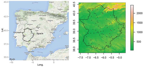
The data used correspond to the extreme rainfall observed at a set of meteorological observatories distributed over the Extremadura region (Spain). Figure 1 shows the location of this region in Spain and the spatial distribution of the observatories considered. The period of study spans from 1961 to 2009. More information about the data selection and the methodology used to obtain the final choice of 72 homogeneous time series can be found in Acero et al. (2017). Due to the strong seasonal character of the rainfall in this region, seasonal maxima were used instead of annual maxima. Seasonal maxima are extracted from the series of daily rainfall at the raingauge in a range of 24 hours. Winter was taken to be December, January and February; spring as March, April and May; and autumn as September, October and November. Summer was not considered because of the low number of rainy events in that season in most parts of Extremadura.

Figure 1. Location of the Extremadura region within the Iberian Peninsula (left). Topographic map of Extremadura together with the locations of the meteorological observatories used in this study (right). The scale is in m a.s.l.

3 Statistical model

As noted in the Introduction, there are several statistical approaches with which to address the problem of spatial extremes. Our choice of a Bayesian approach was motivated by its flexibility, the possibility of adding further elements or layers, and its adaptability to situations in which there appear complex variations in the parameters of the extreme value distribution. However, this kind of model has some drawbacks. One of the most important is that of conditional independence among data observed at different observatories (Davison et al. 2012). Indeed, as will be seen below, such conditional independence is one of the hypotheses of our proposed hierarchical model. Although this is strictly unrealistic since there remain some correlations between data observed at different observatories, in the present case, the seasonal extreme rainfall observed at different observatories may occur on different days, thus reducing the risk of strong correlations. Moreover, as was pointed out by Ribatet et al. (2016) and Davison et al. (2012), unless the goal of the study is to make regional level inferences about future extreme values, a Bayesian hierarchical model is a good choice. Also, the other two approaches do not easily accommodate the incorporation of non-stationary processes.

There has recently arisen a major debate about whether or not to use non-stationary models to fit hydrological time series. See, for example, Milly et al. (2008), who advocate for using non-stationary models, or Montanari and Koutsoyiannis (2014) and Koutsoyiannis and Montanari (2015), who advocate for using stationary models. In the present work, both types of model are proposed and compared with each other. The main hypothesis we posit for using the non-stationary model is that the climate change observed so far may have affected the extreme rainfall in the region under study being a sign the change of the distribution parameters.

In describing the statistical model, we use the usual notation that, for some given random variable X, P(X) represents its probability distribution, and if X₁ and X₂ are two random variables then P(X₁|X₂) represents the conditional probability distribution of X₁ given X₂, and P(X₁,X₂) represents their joint probability distribution. As was mentioned in the Introduction, the statistical model we use is a hierarchical Bayesian model (HBM) of extreme values. To the best of the authors’ knowledge, probably the first time that a HBM formalism was applied to model extreme values was in the paper by Casson and Coles (1999), which studied wind speed extremes along the southeastern coastlines of the United States. Afterwards, the HBM formalism in the context of extreme value analysis was applied by Wikle and Anderson (2003), Renard et al. (2006), Cooley et al. (2007), Sang and Gelfand (2009), Davison et al. (2012), Renard et al. (2013) and Renard and Lall (2014), among others.

The fundamental idea behind hierarchical Bayesian models is that of breaking a complex statistical problem into pieces of more elementary conditional models, estimating the parameters that may appear in them following the Bayesian formalism (Berliner 1996, Wikle et al. 1998, Cressie and Wikle 2011). A useful way to accomplish this task is through the following factorization (Cressie and Wikle 2011):

Stage 1 (data model) P(data | process, parameters)

Stage 2 (process model) P(process | parameters)

Stage 3 (parameter model) P(parameters)

At the first (or data) level, the observed noisy data are assumed to depend on a latent (unknown) process plus several parameters. At the second (process) level, a model is proposed for the latent process through a conditional probability. At the third (parameter) level, probability distributions for the parameters are introduced to take into account their uncertainties. Within the framework of Bayesian statistics, all parameters that appear in the model are considered to be random variables. This allows one to take the uncertainty that appears in the data and in the model into account, in a statistically rigorous manner. Bayes’ theorem allows one to obtain the distribution of the parameters of the model once the data have been observed through the relationship:

(1)

In Bayesian statistics, the distribution on the left-hand side is called the posterior distribution, the distribution P(parameters) to the right is called the prior distribution, and the distribution P(data|process, parameters) is called the likelihood. One of the problems of estimating the parameters through relationship (1) is that of estimating the proportionality constant. This is only feasible in simple problems. However, the introduction of such numerical techniques as the Markov chain Monte Carlo (MCMC) methods (see Gilks et al. 1996) has allowed numerical simulation of the posterior distribution of the parameters, i.e. to obtain a sample of the parameters of interest. In the following subsections, we describe the models used here in more detail.

3.1 First stage

In the first stage, the block extreme data at observatory s are assumed to follow a generalized extreme value (GEV) distribution with probability distribution function:

(2)

where 1 + ξ_s((y − μ_s)/σ_s) ≥ 0. It is also assumed that the block extremes conditional on µ_s, σ_s and ξ_s are spatially and temporally conditionally independent, i.e. the block extreme at observatory s conditional on µ_s, σ_s and ξ_s is independent of the block extreme at observatory s′, and that the block extreme observed at time t is independent of that observed at time t′.

3.2 Second stage

In the second stage, the parameters {µ_s, σ_s, ξ_s}, of the GEV distribution are assumed to be described by a spatio-temporal model, with these parameters being dependent on spatial position s and time t. In spatial data problems, there are three basic types of datasets (Banerjee et al. 2004): (i) point-reference or geostatistical data, where the spatial coordinate s varies continuously over a fixed subset D of Rⁿ; (ii) areal or lattice data, where the domain D is partitioned into a finite numbers of areal units with well-defined boundaries; and (iii) point-pattern data, where D is itself a random set. Our data may be considered as point-reference data since the position of the observatories may be anywhere inside the region of interest. A common model for the spatio-temporal dependence of the GEV parameter is (Wikle et al. 1998, Banerjee et al. 2004):

(3)

where X(s) represents p spatial covariates (geographical coordinates); α_i is a set of p regression parameters; W_i(s, t) is a spatio-temporal model capturing the associations between different sites; _i(s, t) represents the noise not included in the spatio-temporal model (commonly known as the nugget effect), where subscript i represents µ, σ or ξ; s denotes a spatial coordinate; and t is the time. (Recall that, in the framework of Bayesian statistics, µ(s, t), σ(s, t), ξ(s, t), α_i, W_i(s, t) and _i(s, t) are random variables.)

Usually, a Gaussian model independent of the position, i.e. N (0, τ_i ²), is adopted for the pure noise effect _i(s, t). For the spatial covariates X(s), the geographical positions of the observatories are used. However, because the Extremadura region is not large (less than 2° in latitude and longitude and with a total area of 41 632 km²) and part of our interest was to study the effect of the altitude on extreme rainfall, the altitude hs of the observatories was the only covariate chosen. For the spatio-temporal term W_i(s, t), several models were selected. Firstly, a stationary model was fitted, where W_i(s, t) was considered to be a random variable with a Gaussian distribution function, P(W_i(s, t)|·) = N(0, Σ(s, s′, β_i)). For the covariance matrix Σ(s, s′, β_i), an exponential model was chosen:

(4)

where (sill) and (range) are unknown parameters, is the geographical position (longitude, latitude) of the observatory s, and is the distance between the observatories s and s′. In these models, Equation (3) may be regarded as universal kriging with nugget effect (Cressie and Wikle 2011). We were interested not only in the spatial distribution of extreme rainfall over the Extremadura region, but also (probably our main interest) in whether there has been a change in extreme rainfall in time during the period under study. For this reason, a temporal trend was added to the model, but only in the location parameter , whose term now includes a linear temporal trend:

(5)

in which it is assumed that the trend coefficient depends on some covariates in addition to a coefficient that takes into account some spatial correlations (observatories that are geographically close show more similar temporal trends than those that are far away from each other). The altitude of the observatories was taken for the spatial covariate , as in the stationary model. and are two independent geostatistical models similar to those used in the stationary case, i.e. and . Summarizing, the model for the location parameter in the non-stationary case is:

(6)

where and have the same form, with a spatial covariate matrix multiplied by regression coefficients plus a spatially correlated noise. For the scale and shape parameters, the models are the same as in the stationary case (Equation (3)). To close this second stage, the random variables that appear in the left-hand term of Equations (3) are assumed to have a normal distribution:

(7)

Note that this is equivalent to saying that is distributed as .

3.3 Third stage

In the third stage, it is necessary to specify a model for the prior distribution of the different parameters appearing in the model, specifically, the prior distributions of the spatial regression parameters , the spatial model parameters , the variance parameters , and, in the non-stationary case, the trend parameter . In the case of , considering that the only covariate is the altitude of the observatory, each was taken to have a Gaussian distribution:

(8)

where the hyperparameters of mean () and variance () were chosen appropriately in such a way that the distribution was either non- or weakly informative with no extra information about the parameters, e.g. . A similar model (Gaussian) was selected for the trend parameter . Since the normal and inverse gamma distributions are conjugate (Link and Barker 2010), inverse gamma distributions were selected for the sill parameters and . A gamma distribution was chosen for the range parameters .

3.4 Parameter estimation

For the stationary model, from expression (1) and taking into account the hierarchical model introduced in the above subsections, the posterior distribution of the parameters is given by Equation (9):

(9)

where , , and denote the vectors of the GEV parameters at the observatories, denotes the GEV probability density function.

For the non-stationary model, it is given by Equation (10):

(10)

In Equation (10) now represents the vector of GEV parameters at observatory and time , , and represents the time vector .

Note that in the hierarchical models these likelihood functions are built from the probability distributions defined on the first and second stages, and then the prior distribution defined on the third stage is added to obtain the posterior distributions defined on Equations (9) and (10).

The simulation of the posterior distribution was carried out by means of a Markov chain Monte Carlo (MCMC) method, specifically, by using a Gibbs sampler with embedded Metropolis-Hastings steps (see Gilks et al. 1996 for details about the MCMC methods). The theory of MCMC methods shows that, once the Markov chain reaches its stationary distribution, it becomes equal to the posterior distribution, even when the latter is only known up to a normalizing constant (Gilks et al. 1996). This means that it is important to wait for some time until the moment the stationary distribution is attained. This period is known as the “burn-in” period. The problem is that, usually, the number of iterations needed to reach this stationary limit is unknown, and diagnostic tools are necessary to deal with the situation. In the present work, we used the Gelman-Rubin diagnostic convergence test (see Cowles and Carlin 1996 for a review). In this method, several parallel chains initialized from different starting points are run, and convergence is monitored by a parameter called the potential scale reduction factor, which measures the ratio of the between-chain variance to the within-chain variance. When this factor approaches unity, convergence is taken to have been attained. Once the convergence is attained, one gathers the last half of each chain to form a single chain that is used for subsequent calculations. In this work, five chains with 20 000 samples each were run, and a single 50 000 sample chain was formed from these. The Gelman-Rubin diagnostic convergence test was implemented using the CODA (Plummer et al. 2006) package in the R language.

The computer programs used to carry out the simulations were written in FORTRAN. The map figures were prepared using the R packages fields and sp.

3.5 Assessment of goodness of fit of the model

The goodness-of-fit assessment was performed in two stages. In the first stage, several models were fitted to the observed data, and the best one was chosen according to the deviance information criterion (DIC; Spiegelhalter et al. 2014).

This criterion is based on constructing a parameter that takes into account both the “goodness-of-fit” and the “complexity of the model”. The posterior mean of the deviance is used as a measure of the goodness of fit, where the deviance is defined as −2 times the logarithm of the likelihood of the random variable under study, i.e. , with being the vector of parameters of the likelihood, that is, and the GEV density distribution function. The complexity of the model is taken into account by the parameter defined as , which is called the effective number of parameters, where is the deviance at the posterior means of the parameters of interest . The DIC is defined as:

(11)

where the lower the DIC, the better the model. The values of the parameters used to evaluate DIC were obtained during the MCMC evaluation.

In the second stage, the fit of the proposed model was assessed by using the Bayesian posterior predictive distribution (Gelman et al. 1996, Lynch and Bruce 2004). This distribution is used to obtain replicated data , which can be regarded as predictions of the model. If these predictions are not consistent with the observed data in some way, the model can be rejected. Otherwise, one would be disinclined to reject it. The posterior predictive distribution under the hypothesis of conditional independence is given by (Gelman et al. 1996):

(12)

where represents the observed data, is a set of parameters, is the model, corresponds to the distribution under and , and is the posterior distribution under model and observed data . The term could be regarded as the value one might observe in the future under the hypothesis that the model is the same as today, i.e. the prediction. In order to compare these replicated data with the observed ones, some statistic is computed that can represent some features of the data we want the model to reproduce. For example could be the mean, the standard deviation, the maximum, the minimum, etc. A metric quite often used to measure the degree of agreement between the data and the model is the p value, which is defined in the Bayesian context as:

(13)

A value that is too small or too large would indicate that the model does not reproduce the data (or at least some features of the data) well. One way to calculate the value is by means of an MCMC method. As was noted above, an MCMC method allows one to obtain values of the parameter from the posterior distribution . For each simulated value, a value is simulated by using the posited model, and then the discrepancy statistic is computed. Evaluating the number of times that gives the value as:

(14)

where is the number of samples of taken from the Markov chain. It is possible to extend the statistic used in the comparison by incorporating the parameter , i.e. using a statistic for the observed data and for the replicated data. These statistics are termed discrepancy statistics, and, in the case of the observed data, the realized discrepancy (Gelman et al. 1996). The model’s goodness of fit can then be visualized by means of a scatter plot of for each . The proportion of points that are above the 45° line is the value.

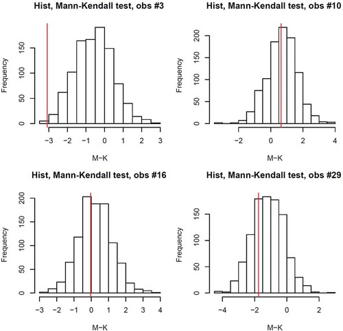
Because of the interest in examining the existence of a temporal trend in the extreme rainfall, a Mann-Kendall test was used as our statistic . For each observatory, we estimated the Mann-Kendall test statistic, using the expression (Gallego et al. 2011):

(15)

where is the sign function defined as if , if , and if ; and n is the number of data for each observatory. Evaluating this statistic for the observed and the replicated data, we calculated the value, and plotted the results as a histogram.

4 Results

4.1 Stationary models

As mentioned above, in a first step and before fitting the whole spatio-temporal model, we fitted a set of stationary models of increasing complexity with the aim of choosing the one that best fits our data. We then introduced into it a temporal trend term to form the spatio-temporal model. The models fitted were the following: Model S0, with no spatial trend in any of the GEV parameters; Model S1, with spatial trend only in the location parameter; Model S2, with spatial trend in location and scale parameters; and Model S3, with spatial trend in the three parameters of the GEV. As also mentioned before, for the spatial trend, the altitude of the observatories was chosen as covariate. It was normalized as:

(16)

where is the altitude above mean sea level of observatory , and and are the maximum and minimum altitudes of the observatories, respectively, so that the new altitude covariate is 0 for the lowest observatory and 1 for the highest. The altitudes of the chosen gauges range from 185 to 796 m a.s.l.

In order to compare the suitability of the four candidate models, the DIC (Section 3.5) was used. The results are presented in Table 1. In winter and autumn, S2 is the best model, and in spring S3. These are therefore chosen as our spatial (stationary) models.

Table 1. Results of using the DIC for the stationary models. Bold indicates the best models.

Model				DIC	Season
S0	28861.38	28687.38	173.99	29035.37	Winter
S1	28859.28	28694.96	164.31	29023.60
S2	28857.88	28693.16	164.72	29022.60
S3	28860.12	28695.93	164.18	29024.30
S0	29831.58	29663.79	167.79	29999.38	Autumn
S1	29832.42	29675.61	156.81	29989.24
S2	29829.69	29673.57	156.12	29985.82
S3	29831.07	29675.69	155.38	29986.45
S0	27000.82	26826.60	174.21	27175.03	Spring
S1	27000.94	26836.21	164.72	27165.67
S2	27000.59	26836.07	164.51	27165.11
S3	26999.54	26835.48	164.06	27163.61

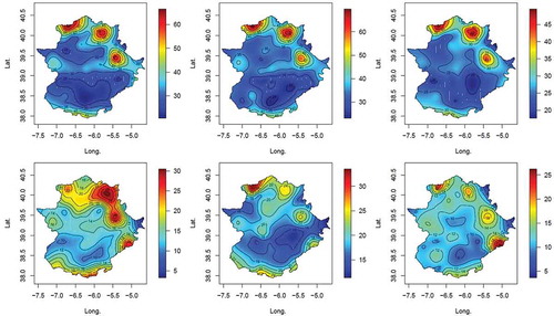
Figure 2 shows the estimated posterior distributions of the spatial trend parameter (α₁) of the chosen models. The spatial trend coefficients (α₁) are clearly positive in the cases of the location and scale parameters (for the latter, what actually appears is the trend in the logarithm of the scale parameter) for all three seasons. The largest value of spatial trend for the location parameter appears in winter, with a mean and standard deviation (SD) of 30.59 and 5.17 mm km⁻¹, respectively. The lowest appears in spring with a mean of 22.11 mm km^–1 (SD: 3.86), and a slightly larger value in autumn with a mean of 24.43 mm km⁻¹ (SD: 4.94). (Note that the units of these estimates are mm km^–1, i.e. they are not normalized.) However, the spatial trend of the scale parameter is quite similar for all three seasons, with a value of about 0.85 km⁻¹ (SD: 0.33 km⁻¹). In the case of spring, for which the S3 model was the best according to the DIC, the spatial trend coefficient for the shape parameter was slightly negative, with a mean of −0.175 km^–1 and SD of 0.295 km^–1. The fact that the location and scale parameter spatial trends are positive is a consequence of the increases in both the amount and variability of the extreme rainfall with altitude. This effect can be seen in Figure 3, in which the highest values of the median appear at the high altitudes in the north and the south of the region, and the lowest values in the river valleys. The pattern is similar for the variances.

Figure 2. Estimated posterior distributions of the spatial-trend coefficients α₁ for location (left), scale (middle), and form (right) parameters for the chosen models: S2 in winter (top row), S2 in autumn (middle row) and S3 in spring (bottom row). The horizontal (red) line shows the 0.025 to 0.975 quantile.

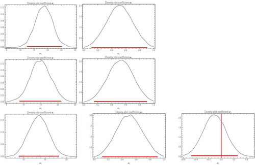
Figure 3. Contour plots of the median (top) and variance (bottom) of the seasonal extreme rainfall for winter (left), autumn (middle) and spring (right).

With the purpose of understanding more clearly the dependence on altitude of the GEV parameters, we have plotted in Figure 4 the means of X(s)·α and X(s)·α + W(s) (the latter includes the error term) in Equation (3) versus the altitude of the observatories.

Figure 4. Plot of the means of the term X(s)·α in Equation (3) versus the altitude of the observatories (in red) and the term X(s)·α + W(s) (black dots), for the location (top), scale (middle) and shape (bottom) parameters, and for winter (left), autumn (middle) and spring (right). The vertical scales are in km, and the horizontal scales in m a.s.l.

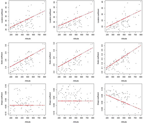
There is a clear positive relationship between both the location and the scale parameters and the altitude of the observatory in the three seasons, even taking the error term W(s) into account. The shape parameter, however, remains nearly constant in winter and autumn, and decreases slightly with altitude in spring. The more negative the shape parameter, the stronger is the tail in the extreme rainfall distribution, so that these results would indicate a stronger tail for the higher observatories in spring.

Another interesting result is the covariance function of the GEV parameters given by Equation (4). Table 2 lists the medians and (2.5, 97.5%) quantiles of the range coefficient β_i1 for the location, scale and shape parameters. The strength of the spatial dependence is similar for the shape and scale parameters, which are nearly three times greater than that of the location parameter. Also, this strength is similar for all three seasons except for the location parameter, for which it is somewhat greater in autumn than in the two other seasons.

Table 2. Median (2.5%, 97.5%) of the range parameters β_i1 for location, scale and shape parameters.

Season	Location	Scale	Shape
Winter	68.2 (35.3, 142.1)	178.1 (91.0, 308.9)	192.1 (99.2, 328.7)
Autumn	84.9 (40.9, 186.4)	188.8 (98.1, 323.7)	200.5 (107.4, 342.0)
Spring	68.3 (33.8, 150.9)	178.6 (92.1, 311.3)	200.8 (108.1, 339.5)

4.2 Non-stationary models

Next, a temporal trend was included in the location parameter of each chosen stationary model (S2 for winter and autumn and S3 for spring). Two temporal trend models were fitted, one without a spatial trend in the time coefficient (T1) and one with it (T2). In other words, in T1, the covariate matrix Y in Equation (6) reduces to a vector column with unit entries, while, in T2, the covariate matrix is a two-column matrix, the first column with unit entries and the second with the observatory altitudes (previously normalized by Equation (16)), specifically:

(17)

Prior to its use in the temporal trend models, the time axis was normalized to the interval (−1, 1).

Table 3 lists the results using DIC. The DIC values are noticeably lower than the values that appear in Table 1, indicating that the temporal trend models are better suited to explaining the data than the stationary ones. The preferred model for winter and autumn is T2, while that for spring is T1.

Table 3. Results of using the DIC for the temporal trend models. Bold indicates the best models.

Model				DIC	Season
T1	26254.82	25096.80	1158.02	27412.84	Winter
T2	25957.06	24740.16	1216.90	27173.97
T1	26926.20	25851.92	1074.28	28000.49	Autumn
T2	26828.26	25749.79	1078.47	27906.73
T1	25893.59	25127.49	766.09	26659.69	Spring
T2	25929.98	25181.07	748.91	26678.90

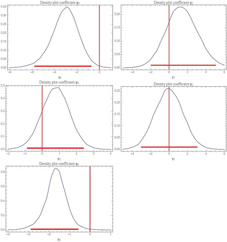
The estimated posterior distributions of the γ coefficients are shown in Figure 5 for the chosen models. For winter, the γ₀ coefficient, which measures the temporal trend of the location parameter at an overall level, is clearly negative. This would indicate that in winter there is a decrease in extreme rainfall over the Extremadura region. The γ₁ coefficient for this season is slightly positive, but the value zero is clearly within the 95% confidence interval around the mean, so that, although the use of the DIC seems to indicate that altitude has an influence on the temporal trend of the location parameter, this influence can be considered as statistically non-significant. For autumn, the distribution of the γ₀ coefficient is preponderantly positive, but not too far from zero, so that one cannot say that there is any increase in extreme precipitation in this season for the region under study. In spring, as in winter, the distribution of the γ₀ coefficient is clearly negative, so that the results would indicate a decrease in extreme rainfall at an overall level in this region.

Figure 5. Estimated posterior distributions of the temporal trend coefficients γ₀ (left) and γ₁ (right) for the chosen models: T2 in winter (top), T2 in autumn (middle) and T1 in spring (bottom). The horizontal (red) line shows the 0.025 to 0.975 quantiles.

In order to evaluate the temporal trend in the location parameter at a local level, we analysed the temporal trend coefficient µ₁(s). Figure 6 shows the means and standard deviations, expressed in mm decade^–1, for the three seasons considered. For the winter, there is a negative temporal trend in the location parameter over the region, except for the more mountainous part in the north. The strongest values correspond to the southeast. The positive values in the more mountainous zone are smaller than those reached in the southeastern zone. For the spring the trend is negative over the whole region but with lower values than those reached in winter. However, in autumn it appears that the location parameter increases with time. The statistical significance of the results was checked by evaluating the p values for each observatory (see Equation (14)) of a zero temporal trend within the distribution of µ₁(s_i) for the ith observatory. The results are shown in Figure 7. The maps show that in autumn (spring), the statistical significance of a positive (negative) temporal trend in the location parameter spans the entire region. In winter, however, only the southeastern negative region appears as statistically significant.

Figure 6. Spatial distributions of the means (top) and standard deviations (bottom) of the temporal trend coefficients µ₁(s) for winter (left), autumn (middle) and spring (right). The scale is in mm decade^–1.

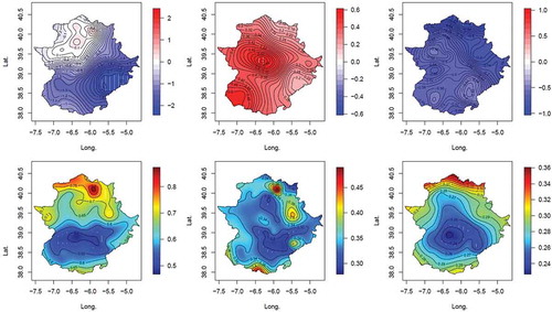
Figure 7. Spatial distributions of the Bayesian p values of the zero value in the temporal trend coefficients µ₁(s) for winter (left), autumn (middle) and spring (right). The isolines 0.025 and 0.05 (autumn) and 0.95 and 0.975 (winter and spring) are shown.

In addition to the regional model for the temporal trend in the extreme rainfall, a local model was fitted for each observatory individually using the Bayesian formulation. In this case the GEV model for each observatory is taken to be:

(18)

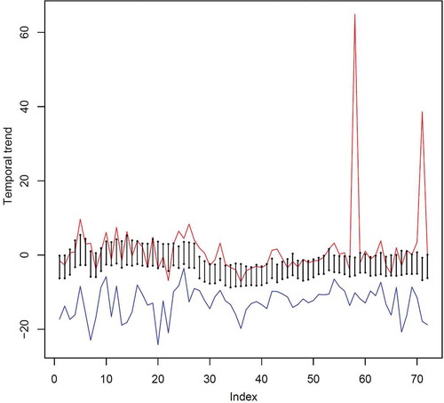
Figure 8 shows for the winter the 2.5 (blue) and 97.5 (red) quantiles of the temporal trend coefficients µ₁ for each local model together with the corresponding quantiles of the regional temporal trend coefficient µ₁(s). Notice that most of the local temporal trends and the regional one are negative. However, the dispersion of the regional temporal trend coefficient is noticeably less than the individual values, so that the use of a regional model has allowed the uncertainty in the evaluation of the temporal trend to be reduced considerably. In this way, the regional model allows the overall tendency of the extreme rainfall over time to be described. This reduction in the uncertainty of the temporal trend was one of the reasons for using a hierarchical spatial model.

Figure 8. Diagram of the quantiles 2.5 (blue) and 97.5 (red) of the temporal trend coefficients µ₁ for each local model together with the corresponding quantiles of the regional temporal trend coefficient µ₁(s) for winter joined by vertical lines.

5 Assessment of the models

As mentioned above, the Mann-Kendall trend test was used to assess the models’ suitability in describing the observed data. To this end, a thousand values of the Markov chain of the fitted model were chosen at random, and from these, a thousand simulated extreme rainfall samples at each observatory were obtained. Figure 9 shows the histograms of the Mann-Kendall statistics of the simulated data together with the Mann-Kendall statistics obtained for the observed data (red line) for four observatories in winter. These examples were selected to show one case with a positive Mann-Kendall statistic (observatory no. 10), one that was negative (observatory no. 29), one nearly zero (observatory no. 16), and one with a p value less than 0.025 (observatory no. 3), which could be considered to be a case in which the model fails to fit the data (or at least this feature of the data by using the Mann-Kendall statistic). Note that the fit could be considered quite good because there is a preponderance of positive values in the histograms when the observed statistic is positive (observatory no. 10), a preponderance of negative values when the observed statistic is negative (observatory no. 29), and a symmetric histogram around the value zero when the observed statistic is close to zero (observatory no. 16). In winter, the model fails to fit the data for eight out of 72 observatories, while in autumn and spring this number falls to only two cases.

Figure 9. Histograms of the Mann-Kendall test statistics of the simulated data together with the Mann-Kendall test statistics of the observed data (red line) for four observatories in winter.

6 Dependence on the North Atlantic Oscillation

The results obtained (discussed in Section 5) support the idea that, during the last 50 years, there has been a decrease in extreme precipitation in Extremadura in the winter and spring seasons and an increase in autumn. A possible cause of this temporal trend is a change in the North Atlantic Oscillation (NAO) pattern during that period. The NAO is the most important mode of variability in the climate of the North Atlantic region and has a major influence on Europe’s climate (Greatbatch 2000). In particular, its influence on precipitation in the Iberian Peninsula has been demonstrated (Rodríguez-Puebla et al. 1998, Goodess and Jones 2002, Trigo et al. 2004, Gallego et al. 2005, Queralt et al. 2009, Casanueva et al. 2014). Within the Iberian Peninsula, the most strongly influenced region is the southwest, which includes the Extremadura region (Rodríguez-Puebla et al. 1998, Goodess and Jones 2002). The canonical view of the NAO is that when it is in its positive state there is reinforcement of the Azores anticyclone, so that many of the storms follow a path to the north of the Iberian Peninsula, with hardly any of the frontal systems passing over the Peninsula, and therefore there is a decrease in rainfall. When it is in its negative phase, however, the weakness of the Azores anticyclone allows more frontal systems to pass over the Iberian Peninsula, thus increasing rainfall over that area. In summary, one expects an increase in precipitation when the NAO is in its negative phase and a decrease when it is in its positive phase. The aforementioned references with respect to the Iberian Peninsula support this conclusion.

In order to explore the influence of the NAO on extreme rainfall, we posited a hierarchical Bayesian model with a GEV distribution, similar to the temporal trend model proposed above, in which the time variable t is replaced by the NAO index. The location parameter is then

(19)

where NAO(t) is the value of the NAO index at time t. This model is analogous to Model T2, but now t is replaced by the NAO index at time t, NAO(t). This NAO(t) index is constructed by averaging the daily NAO index observed at the times the rainfall in the observatories reaches an extreme value in year t. The NAO index is obtained from the Climate Prediction Center (CPC) of the US National Oceanic and Atmospheric Administration.¹ It is based on the first EOF (empirical orthogonal function) of the monthly mean 1000-hPa altitude anomalies poleward of 20° latitude for the Northern Hemisphere.

As before, we fitted two NAO models: NAO1, with the γ coefficients in the expression (19) taken as zero (i.e. the extreme rainfall’s NAO dependence is assumed not to involve the altitude), and NAO2, with the γ coefficients taken to be different from zero (i.e. in which that dependence is assumed to be a function of altitude). Prior to its use in the model, the NAO index was normalized by subtracting its mean for the period under study and dividing by the standard deviation.

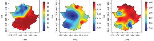
The results using the DIC are presented in Table 4. One may observe that NAO1 is the preferred model for winter, and NAO2 for autumn and spring. The means and standard deviations of the trend coefficients µ₁(s) are displayed in Figure 10, and the Bayesian p values of the zero value in Figure 11. In Figure 10, one may see that, for autumn, there is a negative mean NAO-trend coefficient for most of the Extremadura region, but this could be considered as having “little” statistical significance because the p value of the zero value (see Fig. 11) is less than 95% for the entire region. For spring, except for the southeastern part of the region, the negative NAO-trend coefficient is statistically significant. For winter, most of the region has negative mean NAO-trend values that are statistically significant. There is, however, a singular region in the northeast that has large positive values of both the mean and the standard deviation, but these turn out to not be statistically significant. Given the orders of magnitude difference in the scales in Figure 10, it is clear that the influence of the NAO is much stronger in winter than in the other two seasons. These results are therefore consistent with the expectation that a positive NAO index will lead to a decrease in rainfall in southwestern Spain, especially for winter and to a lesser degree for spring and autumn, probably because the NAO signal is stronger in winter.

Table 4. Results of using the DIC for the NAO-trend models. Bold indicates the best models.

Model				DIC	Season
NAO1	26197.48	25310.53	886.94	27084.42	Winter
NAO2	26278.39	25317.67	960.71	27239.11
NAO1	26826.80	25751.14	1075.66	27902.46	Autumn
NAO2	26814.36	25732.44	1081.91	27896.28
NAO1	25849.06	25075.79	773.26	26622.33	Spring
NAO2	25789.67	24993.46	796.20	26585.88

Figure 10. Spatial distributions of the means (top) and standard deviations (bottom) of the NAO-trend coefficients µ₁(s) for winter (left), autumn (middle) and spring (right).

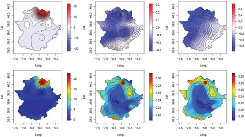
Figure 11. Spatial distributions of the Bayesian p-values of the zero value in the NAO-trend coefficients µ₁(s) for winter (left), autumn (middle) and spring (right). The 0.95 and 0.975 isolines (winter and spring) are shown.

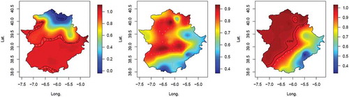
Figure 12. Estimated posterior distributions for the temporal trend coefficients β of a linear temporal regression model of the seasonal NAO index for winter (left), autumn (middle) and spring (right).

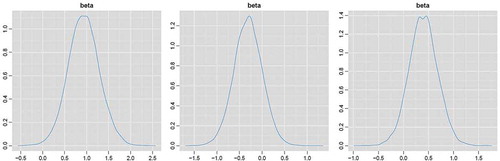
Since the existence of a relationship between the NAO index and the extreme rainfall does not by itself explain the trend observed in the extreme rainfall, it is necessary to see whether there is a trend in the NAO; specifically, it is necessary to examine the relationship between the NAO and the extreme rainfall, and therefore to examine whether the uncertainty in predicting NAO results in a significant increase in the uncertainty of the predictive ability of the model. Figure 12 shows the distributions of the temporal coefficients of a simple linear Bayesian regression model , where (s, t) is a Gaussian noise, and the time is normalized to (0, 1). The results show positive trends for the NAO index in the study period for winter and spring, with mean of the β coefficient of 0.019 year⁻¹ (SD: 0.007 year⁻¹) and 0.008 year⁻¹ (SD: 0.006 year⁻¹), respectively. Autumn, however, has a negative temporal trend with a mean of −0.006 year⁻¹ (SD: 0.006 year⁻¹). The temporal trend is thus more marked in winter than in spring or autumn.

One may conclude from these results that the increase in the NAO index for winter and spring could have led to the decrease observed in extreme rainfall events over Extremadura during the study period (1961–2009). Nonetheless, the lack of any clear relationship between the NAO and extreme rainfall in autumn together with the weak trend observed for the NAO in this season preclude us from attributing the observed increase in extreme rainfall in autumn to the variation of the NAO during that season for the period under study.

7 Summary and conclusions

In this work, we have presented a statistical study of extreme rainfall in the region of Extremadura during the second half of the 20th century. For this purpose, we used a hierarchical spatio-temporal Bayesian model with a GEV parameterization of the extreme event data. This use of a hierarchical model allowed us to pool the spatial information straightforwardly and consistently. Due to the seasonal character of precipitation in this geographical region, the study was carried out independently for each of three seasons: winter, autumn and spring. Summer was ignored due to the lack of precipitation in that season. The study was performed in two steps. In the first step, spatial models were selected for location, scale and shape parameters. In the second, a temporal trend term was introduced in the location parameter as a way to take into account the influence of climate change on the region’s extreme rainfall. The deviance information criterion was used to select the best model.

The results show that, for the Extremadura region over the period 1961–2009, there had been a decrease in extreme rainfall in winter and spring and a slight increase in autumn. These findings are consistent with other studies of extreme rainfall over the Iberian Peninsula (García et al. 2007, Acero et al. 2011). Comparison of the hierarchical model results with those obtained by fitting a GEV distribution locally showed the former to have led to markedly lower uncertainties in the trend parameters.

We found a negative relationship between the NAO index and Extremadura’s extreme rainfall in winter. In spring and autumn, however, the results were less conclusive, probably because the NAO index is weaker in those two seasons. We also found an increase in the intensity of the NAO index in winter and spring, and a slight decrease in autumn. The increase in winter could help explain this season’s reduction in extreme rainfall in our region.

Acknowledgements

We thank the co-editor, associate editor and the two reviewers for comments and suggestions which we believe have greatly improved both the readability and the content of this paper. Thanks are also due to the developers of the R statistical packages field and sp used in this work to prepare the map figures.

Disclosure statement

No potential conflict of interest was reported by the authors.

Additional information

Funding

Support from the Junta de Extremadura-FEDER Funds through Research Group Grants [GR15137], Junta de Extremadura-Consejería de Economía e Infraestructuras [FEDER Funds IB16063] and from the Ministerio de Economía y Competitividad through Group Grants [MTM2014-56949-C3-3-R] is gratefully acknowledged.

Notes

¹ http://www.cpc.ncep.noaa.gov/products/precip/CWlink/pna/nao.shtml Refer to this web page for more information on the procedure used by the CPC to obtain the index.

References

- Acero, F.J., et al., 2017. Non-stationary future return levels for extreme rainfall over Extremadura (SW Iberian Peninsula). Hydrological Sciences Journal, 62 (9), 1394–1411. doi:10.1080/02626667.2017.1328559
- Acero, F.J., García, J.A., and Gallego, M.C., 2011. Peaks-over-threshold study of trends in extreme rainfall over the Iberian Peninsula. Journal of Climate, 24 (3), 1089–1105. doi:10.1175/2010JCLI3627.1
- Aryal, S.K., et al., 2009. Characterizing and modeling temporal and spatial trends in rainfall extremes. Journal of Hydrometeorology, 10, 241–253. doi:10.1175/2008JHM1007.1
- Banerjee, S., Carlin, B.E., and Gelfand, A.E., 2004. Hierarchical modeling and analysis for spatial data. New York: Chapman & Hall.
- Berliner, M.L., 1996. Hierarchical Bayesian time series. New York: Springer.
- Casanueva, A., et al., 2014. Variability of extreme precipitation over Europe and its relationships with teleconnection patterns. Hydrology and Earth System Sciences, 18, 709–725. doi:10.5194/hess-18-709-2014
- Casson, E. and Coles, S., 1999. Spatial regression models for extremes. Extremes, 1 (4), 449–468. doi:10.1023/A:1009931222386
- Cooley, D., Nychka, D., and Naveau, P., 2007. Bayesian spatial modeling of extreme precipitation return levels. Journal of the American Statistical Association, 102 (479), 824–840. doi:10.1198/016214506000000780
- Cowles, M.K. and Carlin, B.P., 1996. Markov chain Monte Carlo convergence diagnostics: a comparative review. Journal of the American Statistical Association, 91 (434), 883–904. doi:10.1080/01621459.1996.10476956
- Cressie, N., and Wikle, C.K., 2011. Statistics for spatio-temporal data. New York: Wiley.
- Davison, A.C., Padoan, S.A., and Ribatet, M., 2012. Statistical modeling of spatial extremes. Statistical Science, 27 (2), 161–186. doi:10.1214/11-STS376
- Dyrrdal, A.V., et al., 2015. Bayesian hierarchical modeling of extreme hourly precipitation in Norway. Environmetrics, 26 (2), 89–106. doi:10.1002/env.2301
- Epstein, E.S., 1985. Statistical inference and prediction in climatology: a Bayesian approach. Boston, MA: American Meteorological Society, Meteorological Monographs 20.
- Gaetan, C. and Grigoletto, M., 2007. A hierarchical model for the analysis of spatial rainfall extremes. Journal of Agricultural, Biological and Environmental Statistics, 12 (4), 434–449. doi:10.1198/108571107X250193
- Gallego, M.C., et al., 2011. Trends in frequency indices of daily precipitation over the Iberian Peninsula during the last century. Journal of Geophysical Research, 116, D02109. doi:10.1029/2010JD014255
- Gallego, M.C., García, J.A., and Vaquero, J.M., 2005. The NAO signal in daily rainfall series over the Iberian Peninsula. Climate Research, 29, 103–109. doi:10.3354/cr029103
- García, J.A., et al., 2007. Trends in block-seasonal extreme rainfall over the Iberian Peninsula in the second half of the twentieth century. Journal of Climate, 20, 113–130. doi:10.1175/JCLI3995.1
- Gelman, A., Meng, X.L., and Stern, H., 1996. Posterior predictive assessment of model fitness via realized discrepancies (with discussion). Statistica Sinica – Journal, 6, 733–807.
- Gilks, W.R., Richardson, S., and Spiegelhalter, D.J., 1996. Introducing Markov Chain Monte Carlo. In: Markov Chain Monte Carlo in practice. New York: Chapman & Hall.
- Goodess, C.M. and Jones, P.D., 2002. Links between circulations and changes in the characteristics of Iberian rainfall. International Journal of Climatology, 22, 1593–1612. doi:10.1002/joc.810
- Greatbatch, R.J., 2000. The North Atlantic oscillation. Stochastic Environmental Research and Risk Assessment, 14, 213–242. doi:10.1007/s004770000047
- Koutsoyiannis, D. and Montanari, A., 2015. Negligent killing of scientific concepts: the stationarity case. Hydrological Sciences Journal, 60, 1174–1183. doi:10.1080/02626667.2014.959959
- Link, W.A., and Barker, R.J., 2010. Bayesian inference with ecological applications. San Diego, CA: Academic Press.
- Lynch, S.M. and Bruce, W., 2004. Bayesian posterior predictive checks for complex models. Sociological Methods & Research, 32, 301–335. doi:10.1177/0049124103257303
- Milly, P.C.D., et al., 2008. Stationarity is dead: whither water management? Science, 319, 573–574. doi:10.1126/science.1151915
- Min, S.-K., et al., 2011. Human contribution to more-intense precipitation extremes. Nature, 470, 378–381. doi:10.1038/nature09763
- Montanari, A. and Koutsoyiannis, D., 2014. Modeling and mitigating natural hazards. Stationarity is Immortal! Water Resources Research, 50, 9748–9756. doi:10.1002/2014WR016092
- Pall, P., et al., 2011. Anthropogenic greenhouse gas contribution to flood risk in England and Wales in autumn 2000. Nature, 470, 382–385. doi:10.1038/nature09762
- Plummer, M., et al., 2006. CODA: convergence diagnosis and output analysis for MCMC. R News, 6, 7–11.
- Queralt, S., et al., 2009. North Atlantic oscillation influence and weather types associated with winter total and extreme precipitation events in Spain. Atmospheric Research, 94, 675–683. doi:10.1016/j.atmosres.2009.09.005
- Ragulina, G. and Reitan, T., 2017. Generalized extreme value shape parameter and its nature for extreme precipitation using long time series and the Bayesian approach. Hydrological Sciences Journal, 62 (6), 863–879. doi:10.1080/02626667.2016.1260134
- Renard, B., 2011. A Bayesian hierarchical approach to regional frequency analysis. Water Resources Research, 47, W11513. doi:10.1029/2010WR010089
- Renard, B., Garreta, V., and Lang, M., 2006. An application of Bayesian analysis and Markov chain Monte Carlo methods to the estimation of a regional trend in annual maxima. Water Resources Research, 42, W12422. doi:10.1029/2005WR004591
- Renard, B. and Lall, U., 2014. Regional frequency analysis conditioned on large-scale atmospheric or oceanic fields. Water Resources Research, 50, 9536–9554. doi:10.1002/2014WR016277
- Renard, B., Sun, X., and Lang, M., 2013. Bayesian methods for non-stationary extreme value analysis. In: A. AghaKouchak, et al., eds. Extremes in a changing climate: detection, analysis and uncertainty. Water Science and Technology Library. New York: Springer, 39–95.
- Ribatet, M., Dombry, C., and Oesting, M., 2016. Spatial extremes and max-stable processes. In: D.K. Dey and J. Jan, eds. Extreme value modeling risk analysis, methods and applications. New York: CRC Press, 179–194.
- Rodríguez-Puebla, C., et al., 1998. Spatial and temporal patterns of annual precipitation variability over the Iberian Peninsula. International Journal of Climatology, 18, 299–316. doi:10.1002/(SICI)1097-0088(19980315)18:3<299::AID-JOC247>3.0.CO;2-L
- Sang, H. and Gelfand, A.E., 2009. Hierarchical modeling for extreme values observed over space and time. Environmental and Ecological Statistics, 16, 407–426. doi:10.1007/s10651-007-0078-0
- Spiegelhalter, D.J., et al., 2014. The deviance information criterion: 12 years on. Journal of the Royal Statistical Society B, 76, 485–493. doi:10.1111/rssb.12062
- Sun, X., et al., 2014. A general regional frequency analysis framework for quantifying local-scale climate effects: a case study of ENSO effects on Southeast Queensland rainfall. Journal of Hydrology, 512, 53–68. doi:10.1016/j.jhydrol.2014.02.025
- Trigo, R.M., et al., 2004. North Atlantic oscillation influence on the precipitation river flow and water resources in the Iberian Peninsula. International Journal of Climatology, 24, 925–944. doi:10.1002/joc.1048
- Viglione, A., et al., 2013. Flood frequency hydrology: 3. A Bayesian analysis. Water Resources Research, 49 (2), 675–692. doi:10.1029/2011WR010782
- Wikle, C.K. and Anderson, C.J., 2003. Climatological analysis of tornado report counts using a hierarchical Bayesian spatio-temporal model. Journal of Geophysical Research, 108, 9005. doi:10.1029/2002JD002806
- Wikle, C.K., Berliner, M.L., and Cressie, N., 1998. Hierachical Bayesian space-time models. Environmental and Ecological Statistics, 5, 117–154. doi:10.1023/A:1009662704779