Evaluation of four hydrological models for operational flood forecasting in a Canadian Prairie watershed

ABSTRACT

The complexities of the Prairie watersheds, including potholes, drainage interconnectivities, changing land-use patterns, dynamic watershed boundaries and hydro-meteorological factors, have made hydrological modelling on Prairie watersheds one of the most complex task for hydrologists and operational hydrological forecasters. In this study, four hydrological models (WATFLOOD, HBV-EC, HSPF and HEC-HMS) were developed, calibrated and tested for their efficiency and accuracy to be used as operational flood forecasting tools. The Upper Assiniboine River, which flows into the Shellmouth Reservoir, Canada, was selected for the analysis. The performance of the models was evaluated by the standard statistical methods: the Nash-Sutcliffe efficiency coefficient, correlation coefficient, root mean squared error, mean absolute relative error and deviation of runoff volumes. The models were evaluated on their accuracy in simulating the observed runoff for calibration and verification periods (2005–2015 and 1994–2004, respectively) and also their use in operational forecasting of the 2016 and 2017 runoff.

KEYWORDS:

• Prairie watershed
• hydrological model
• hydrological forecasting
• Shellmouth basin
• hydrological forecast centre
• hydrological model evaluation

Editor R. Woods Associate editor N. Verhoest

1 Introduction

Flooding is the most common and costliest natural disaster in Canada, claiming more than 200 human lives and causing over CAD 2 billion in damage during the 20th century (Jakob and Church 2011, Buttle et al. 2016). Canadian Prairie provinces have experienced significant floods in the past 20 years ranging from mid-range to historic record floods. The 2013 flood in Alberta, the 2011 and 2014 floods in Manitoba, and the 2013 flood in Saskatchewan are a few of the recent examples that caused infrastructural damage costing billions of dollars. The 2013 flood in Alberta was the second-costliest natural disaster in Canadian history, with flood damage losses and recovery costs exceeding CAD 6 billion (Burn and Whitfield 2016, Pomeroy et al. 2016). The cost of the 2011 flood in Manitoba was estimated to be CAD 1.2 billion (Manitoba Infrastructure and Transportation 2013, Burn and Whitfield 2016).

In an attempt to control floods and mitigate future flood damages in the Prairie provinces, provincial and federal governments have initiated various task forces to review the past floods. In Manitoba, the 2011 Flood Review Task Force was established to assess the cause of the 2011 flood, flood recovery procedures and flood forecasting methodologies (Manitoba Infrastructure and Transportation 2013). A similar task force was established in Alberta following the 2013 historic flood (Flood Recovery Task Force 2013, Alberta WaterSMART 2013). Both these task forces evidently suggested that accurate and timely flood forecasting is essential to protect lives and property (Flood Recovery Task Force 2013, Manitoba Infrastructure and Transportation 2013). Accurate flood forecasting and effective communication, with timely dissemination of warning information to the public and authorities, can minimize the economic and social impacts of floods to communities and can result in measures that will enhance ecological conditions (Penning-Rowsell et al. 2000, Carsell et al. 2004). Accurate flood forecasting and early flood warning could avoid or significantly reduce the damage caused by flooding (Parker et al. 2005, Pappenberger et al. 2015). The UK Environment Agency performed benefit–cost analysis of flood forecasting and warning response systems (FFWRS) in England and Wales, and the results of the analysis showed that accurate flood forecasting could have a benefit–cost ratio of 4.82 for an investment in accurate flood forecasting (Environment Agency 2003, Parker et al. 2005).

The purpose of this study is to examine various hydrological models in order to determine whether one hydrological model is sufficient to be used as a main forecasting model in a Prairie watershed. We looked at four hydrological models ranging from complex fully distributed models to relatively simple lumped models. The models were developed, calibrated and tested for their efficiency and accuracy to be used as operational flood forecasting tools at the Manitoba Hydrologic Forecasting Centre.

2 Complexity of Prairie watersheds for hydrological modelling

2.1 Watershed characteristics

The Prairie region of Canada lies in the southern part of the provinces of Alberta, Saskatchewan and Manitoba, and is a portion of the Northern Great Plains of North America (Fang et al. 2007). The region is characterized by numerous glacially formed depressions, which fill with water to form potholes, sloughs, wetlands and dugouts (Pomeroy et al. 2005, Fang et al. 2007). These depressions are very important to prairie hydrology due to their surface storage capacity, and they can significantly influence runoff response and timing (Fang et al. 2007). Because of poorly developed stream networks, much of the prairie land does not normally drain (contribute) to any stream or river system (Godwin and Martin 1975, Pomeroy et al. 2005), resulting in closed catchments (Hayashi et al. 2003), which are also defined as non-contributing areas. Therefore, on the Prairies, there is a significant difference between the gross drainage area and the effective drainage area. The gross drainage area is delineated based on topography and is expected to contribute runoff to the main channel under extremely wet conditions. The gross drainage area is divided into the effective drainage area, which contributes runoff to the main stream during a flood with a return period of 2 years, and the non-contributing area, which does not contribute runoff (Godwin and Martin 1975, Pomeroy et al. 2005).

2.2 Prairie hydrology

In addition to the watershed complexity, hydrology in the Canadian Prairie region is also complex and highly variable (Fang et al. 2007). Surface runoff water generated from the basin during snowmelt and heavy rainfall remains stored in depressions until the surface storage is filled. After the storage volume is satisfied, additional surface water spills and flows to the wetlands and lakes further downstream, eventually reaching the outlet. This results in a sporadic and rapid increase in contributing area during peak runoff events (Fang et al. 2007). During dry years, the water stored in sloughs provides input to local groundwater systems in excess of that available from precipitation, while in wet years, the storage of water in the sloughs helps to reduce flood peaks (Pomeroy et al. 2005, Fang et al. 2007). In addition, Prairie wetlands are important for wildlife, aesthetics, groundwater recharge and small-scale water supplies (Pomeroy et al. 2005).

2.3 Frozen ground effect

Another complexity of the Prairies area is the effect of frozen ground conditions during the snowmelt period. The Prairies is a cold region and exhibits classical cold region hydrology, with continuous snow cover and frozen soils over much of the region in the winter (Pomeroy et al. 2007). Since the soils are frozen, rapid snowmelt runoff occurs in the springtime, producing more than 80% of annual local runoff (Gray and Landine 1988, Fang et al. 2007). The amount of runoff generated from snowmelt during spring periods is strongly dependent on the rate of infiltration through frozen ground. The clay-rich soils of the prairies have low hydraulic conductivity and even lower when they are frozen (Zhao and Gray 1997, Pomeroy et al. 1998, Hayashi et al. 2003). Infiltration of snowmelt water into frozen soils is a complicated process affected by many factors including the hydro-physical and thermal properties of the soil, soil moisture and temperature regimes, the rate of release of meltwater from the snow cover, and the energy content of the infiltrating water (Granger et al. 1984, Pomeroy et al. 1998, Gray et al. 2001).

2.4 Land-use change

Due to the aridity and gentle topography of the Prairies, natural drainage systems are poorly developed, disconnected and sparse. This results in surface runoff that is both infrequent and spatially restricted (Gray 1970, Fang et al. 2007). However, recent artificial drainage activities have increased runoff to streams and wetlands in some regions. Land cover also exerts great control on the prairie hydrology and is an essential factor affecting the snow accumulation process (Fang et al. 2007, Dumanski et al. 2015). In addition to hydro-meteorological factors, uncertainty due to fill and spill of the surface depression storages and the separation of contributing and non-contributing areas to the streamflow create complexity for successful modelling.

3 Models selected for the assessment

Four hydrological models ranging from fully distributed models to a simple lumped model were selected and examined for efficiency of operational flood forecasting. The hydrological models were primarily developed to forecast inflow into Shellmouth Reservoir, which is a multi-purpose reservoir providing flood control, water supply, irrigation and recreational benefits in the Prairies region.

3.1 WATFLOOD model

The WATFLOOD model is a partially physically-based, distributed hydrological model which has been widely used for flood forecasting and long-term hydrological simulation using distributed precipitation data from radar or numerical weather models (Kouwen 2016). The model was first introduced in 1973 (Kouwen 1973). The processes modelled include interception, infiltration, evaporation, snow accumulation and ablation, interflow, recharge, baseflow, and overland and channel routing (Kouwen 1988, Kouwen et al. 1993, Neff 1996). WATFLOOD implements a grouped response unit (GRU) approach and subdivides segments according to the similarity of hydrological responses. A GRU is a conceptual grouping of land surface areas with similar land use that are expected to have similar hydrological response. The runoff response from each unit with an individual land-cover make-up and topography (elevation) is calculated and routed downstream (Cranmer et al. 2001, Jenkinson 2009, Kouwen 2016). River channels are classified in a similar manner to land classes. WATFLOOD computes infiltration using the Philip formula (Philip 1954), which represents physical aspects of the infiltration process. WATFLOOD uses Green Kenue as a pre- and post-processor. Green Kenue is a GIS-based data preparation, analysis and visualization tool for hydrological modellers developed by the Canadian Hydraulics Centre, CHC (Canadian Hydraulics Centre 2010). There are additional programs for data pre-processing, such as RAGMET.exe and TMP.exe, which are used to distribute precipitation and temperature data from weather stations and convert to the square grid to be used in the model. Further details of the WATFLOOD model can be found in Kouwen (2016).

3.2 HBV-EC model

The HBV (Hydrologiska Byråns Vattenbalansavdelning) model is a conceptual model of catchment hydrology, which was originally developed by Lindström et al. (1997) at the Swedish Meteorological and Hydrological Institute. The version of the model used in this study is the HBV-EC model, which is a Canadian version of the HBV-96 model (Lindström et al. 1997). HBV-EC is a partially distributed conceptual model that simulates streamflow using daily precipitation, air temperature, and long-term monthly potential evaporation (Bergström 1995, Hamilton et al. 2000, Zegre 2008). The HBV-EC model is distributed because basins are divided into sub-catchments and conceptual processes are distributed by vegetation and vegetation zones. The model consists of three components: a snow routine for snow accumulation and snowmelt based on the degree-day method; a soil routine that controls the proportion of rainwater and snowmelt, which generates excess water after considering soil moisture and evaporation requirements; and a runoff generation routine consisting of an upper, nonlinear reservoir that represents fast discharge and a lower linear reservoir that represents slow discharge or baseflow (Zegre 2008, Grillakis et al. 2010). The HBV-EC model is also run through Green-Kenue (CHC 2010). HBV-EC is based on the concept of grouped response units (GRUs), which contain grid cells having similar elevation, aspect, slope, and land cover (Mahat and Anderson 2013). It has the capability to model four land-cover types: open, forest, glacier and water (Jost et al. 2012). To represent lateral climate gradients, HBV-EC allows a basin to be subdivided into different climate zones, each of which is associated with a single climate station and a unique parameter set (Jost et al. 2012). Detailed descriptions of the HBV hydrological model are found in (Bergström 1995, Lindström et al. 1997, Zhang and Lindström 1997, Hamilton et al. 2000, Hundecha and Bárdossy 2004).

3.3 HEC-HMS model

The Hydrologic Modeling System (HEC-HMS) is a hydrological modelling software developed by the Hydrologic Engineering Center of the US Army Corps of Engineers (USACE-HEC 2016). HEC-HMS is a physically based and conceptual lumped model designed to simulate complete hydrological processes of dendritic watersheds in space and time (Feldman 2000, USACE-HEC 2015, 2016). HEC-HMS uses separate models to represent each component of the runoff process. The meteorological component is the first computational unit by which precipitation input is spatially and temporally distributed over the basin. The precipitation is subject to losses modelled by the precipitation loss component (Feldman 2000, Cunderlik and Simonovic 2004). The resulting excess precipitation contributes either to direct runoff, modelled by a direct runoff component which is transferred to overland flow, or to groundwater flow, modelled by a baseflow component (Feldman 2000, Mousavi et al. 2012). The overland flow and baseflow enter river channels, and the translation and attenuation of flow are simulated by the river routing component (Cunderlik and Simonovic 2004). Finally, the effect of reservoirs, detention basins and natural depressions, such as lakes, ponds and wetlands, is computed by the reservoir component (Feldman 2000). The soil moisture accounting (SMA) algorithm in HEC-HMS accounts for a watershed’s soil moisture balance over a long-term period and is suitable for simulating daily, monthly and seasonal streamflows (Chu and Steinman 2009).

3.4 HSPF model

The Hydrologic Simulation Program-Fortran (HSPF) is a continuous simulation conceptual hydrological model, which uses a version of the Stanford Watershed Model developed in the early 1960s by Crawford and Linsley (1966), and further developed and improved in the 1980s by the US Environmental Protection Agency (Donigian et al. 1984). Detailed description of the HSPF model is provided in the HSPF Version 12.2 User’s manual (Bicknell et al. 2005). HSPF can simulate the hydrological processes and associated water quality processes on pervious and impervious land surfaces, and in streams and reservoirs at user-specified spatial and temporal scales. The input data time step of the model ranges from sub-hourly to monthly, and model analysis could be done for hundreds of years. HSPF simulates interception, soil moisture, surface runoff, interflow, baseflow, snowpack depth and water content, snowmelt, evapotranspiration, groundwater recharge, and channel and reservoir routings (USGS 1997). It uses conceptual storages to distribute the incoming precipitation into canopy interception, surface detention, and upper zone and lower zone storages. Channel inflow is routed by hydrological routing technique to account for attenuation and translation of the storage effect of the channel. The energy balance and degree-day methods are the two options available for modelling snow accumulation and snow melt from sub-basins in HSPF (Bicknell et al. 2005). HSPF is public-domain software with worldwide practical application for more than 30 years. Some of the applications and uses of HSPF include the effects of land-use change and climate change assessments, flow diversions, flood control planning and operations.

4 Study area and input data

4.1 Shellmouth Reservoir basin

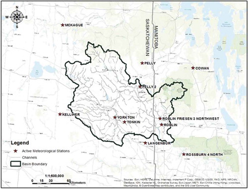
The Shellmouth Reservoir basin is part of the Upper Assiniboine River basin, with a total drainage area of 17 900 km². The Assiniboine River and its tributaries are located in eastern Saskatchewan and western Manitoba, Canada. Most of the basin lies within what is often called the prairie pothole region, a 750 000 km² area in the Prairie and Parkland regions covering portions of southern Manitoba, Saskatchewan, Alberta, and North and South Dakota (Upper Assiniboine River Basin Study Report 2000). The geomorphology of the basin is characterized by numerous shallow potholes or sloughs. These potholes, in some portions of the basin, cover 10–20% of the landscape (Upper Assiniboine River Basin Study Report 2000). Many of the potholes are very shallow and only retain spring runoff for a limited period. The presence of potholes creates intermittent flow in the catchment, and the existence of a number of lakes and the complex dynamics of the wetlands are the main characteristics of the Upper Assiniboine River basin (Upper Assiniboine River Basin Study Report 2000, Muhammad et al. 2016). Figure 1 shows the Shellmouth basin and 11 active meteorological stations selected for the models.

Figure 1. The Shellmouth basin, Canada.

4.2 Soil type

Soil type in a watershed influences hydraulic conductivity, porosity and other soil parameters, such as saturation and field capacity. The soil parameters also determine water storage and runoff in the unsaturated zone of the soil. These parameters are critical in determining the amount of water that can be stored in the soil, and how much of it can be converted to runoff and flow into surface watercourses. Black chernozemic soils overlay almost 70% of the Shellmouth Reservoir basin (Upper Assiniboine River Basin Study Report 2000). These soils are high in organic matter and have generally developed under native grassland vegetation. In the northern and southwestern portions of the basin, the black soils have been modified to dark grey and grey chernozemic and luvisolic soils. Regosolic soils generally occur in river valleys and adjacent to basin lakes. These soils are light-coloured, lack distinct horizons and are highly fertile as a result of alluvial deposition during periodic flood events (Upper Assiniboine River Basin Study Report 2000).

4.3 Land cover

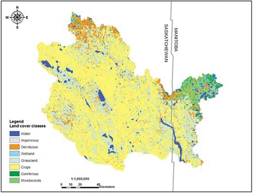
Land-cover information was obtained from the Natural Resources Canada (NRCan) GeoGratis dataset (http://www.nrcan.gc.ca/earth-sciences/resources/10778). There are 21 different land classes in the raw shapefiles obtained from GeoGratis. To reduce the number of land classes for the simplicity of modelling, similar land-cover classes were combined into various common land classes such as crops, grassland, wetland, water etc., as needed by the individual model. The most dominant land-cover class in the basin is cropland, covering 55% of the basin, followed by grassland (24%) and forest (14%). Water bodies and wetlands cover 4.2 and 1.4% of the basin, respectively. Several naturally occurring lakes are also found in the basin, most notably the Good Spirit and Fishing lakes. The prairie wetlands in the basin serve a number of functions in the hydrological cycle. Wetlands usually act as large sponges or dampers within a watershed, temporarily storing runoff and releasing excess water in a slow, controlled manner. This natural process reduces the magnitude of downstream flooding in most years (Upper Assiniboine River Basin Study Report 2000). Figure 2 shows the combined land cover for the watershed. Over the past century, the landscape of the basin has undergone extensive changes (Upper Assiniboine River Basin Study Report 2000). Most of the natural prairie and parkland has been converted into agricultural land for crop production.

Figure 2. Combined land cover for the Shellmouth basin.

4.4 Digital elevation model

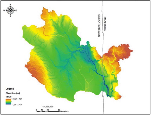
The digital elevation model (DEM) information was obtained from NRCan’s GeoGratis website. The raw DEM was processed using GIS and channels and sub-basin characteristics were extracted from the DEM. The topography of the basin is gently to moderately undulating with the higher relief evident in the northeastern portion of the basin. The elevation in the basin ranges from a high of 791 m a.s.l. to a low of 364 m a.s.l. The DEM of the Shellmouth basin is shown in Figure 3.

Figure 3. Digital elevation model (DEM) of the Shellmouth basin.

4.5 Hydro-meteorological data

Historical daily climate data for various stations across the basin within Manitoba and Saskatchewan were obtained from the Environment Canada metrological stations. After thorough analysis of data quality and quantity, 11 active meteorological stations were selected covering the period from 1994 to 2016 (Figs 1 and 4). Daily precipitation and temperature data were retrieved for the stations and data quality checks were performed. Missing values were filled by interpolating from nearby stations and also using the area ratio method. The climate of the basin is continental sub-humid, characterized by long, cold winters and short, warm summers (Upper Assiniboine River Basin Study Report 2000). Based on the recorded gauged data, the annual average precipitation in the basin is about 520 mm.

Figure 4. Sub-basins of Shellmouth basin, and hydrometric and meteorological stations.

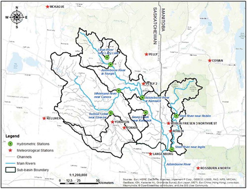
There are eight streamflow gauges (hydrometric stations) incorporated within the model. Streamflow data for these stations were obtained from Water Survey of Canada. Recorded streamflow data are required in the model to calibrate various model parameters and to verify the model. The total inflow into the reservoir is computed based on recorded reservoir levels, the elevation–storage curve of the reservoir, and the outflow from the reservoir for a specified gate setting. Figure 4 shows the meteorological stations and streamflow gauges used in the models and the corresponding sub-basins.

5 Model calibration and verification

Calibration is the process of fine tuning model parameters to increase the predictive accuracy of a model. Model parameters are changed in a systematic way and the model is run repeatedly until the simulated flows match measured values within a range that is considered acceptable. The models were calibrated and validated on runoff at a daily time step. All models were calibrated on a 10-year dataset (2005–2015) and validated on another 10-year dataset (1994–2004). The first years in both calibration and validation were used as a spin-up period in order to stabilize the model and obtain representative initial conditions. Some of the main parameters adjusted for model calibration included channel roughness, soil permeability, soil retention, overland flow roughness, melt factor, base temperature and a sublimation factor. Automatic calibration and the use of Monte Carlo simulation was conducted in most models to obtain the best calibration parameters. Selected calibrated parameters for the four models are shown in Tables 1–4. Once the models were calibrated, a verification (validation) simulation was conducted. Model verification (validation) is the process of determining the degree to which the model represents the process accurately and is capable of giving acceptable results for the intended uses of the model, without changing the model parameters obtained from the calibration. To verify the calibrated model, a separate independent set of data was used to compare modelled and observed flows. The results of calibration and validation for the WATFLOOD, HSPF, HBV-EC and HEC-HMS models are presented in Figures 5 and 6, respectively.

Table 1. Calibrated parameters for the WATFLOOD model. Ass.: Assinboine; Kam.: Kamsak; Sturg.: Sturgis (see Fig. 4 for locations).

Routing parameters	River name
	Stony Creek	Shell River	Yorkton Creek	Ass. at Kam.	Lilian River	Ass. at Sturg.	White-sand
Lower zone coefficient	0.0001	0.0031	0.0050	0.0009	0.0023	0.0047	0.0049
Lower zone exponent	0.86	1.48	0.72	0.33	2.47	1.11	0.62
Overbank Manning’s n	0.4	0.4	0.7	0.4	0.4	0.4	0.4
Channel Manning’s n	0.074	0.056	0.075	0.070	0.039	0.014	0.067
Wetland or bank porosity	0.8	1	0.9	0.9	0.2	0.4	0.7
Hydrological and snow parameters	Land-cover type
	Crop	Grass	Deciduous	Coniferous	Mixed	Wetland	Water
Interflow coefficient	0.53	1.93	9.67	4.85	8.87	3.32	0.10
Infiltration coefficient, bare ground	35.7	35.4	40.6	31.3	41.6	303.0	0.0
Infiltration coefficient, snow covered	0.11	0.25	0.02	0.48	0.04	0.27	0.00
Upper zone retention (mm)	97.0	97.7	40.9	14.3	144	84.9	144
Recharge coefficient, bare ground	0.16	0.29	0.01	0.24	0.07	0.08	0.07
Melt factor (mm °C^−1 h^−1)	0.11	0.08	0.08	0.16	0.11	0.10	0.10
Base temperature (°C)	0	−1.2	−3.0	−3.2	−0.03	−3.1	−0.5
Sublimation rate (mm d^−1)	1.27	1.47	0.37	0.24	0.08	0.25	0.16

Table 2. Calibrated parameters for the HBV-EC model.

Parameter	Definition	Calibrated value
ForestTFRAIN	Fraction of rainfall reaching ground surface below forest	0.8
ForestTFSNOW	Fraction of snowfall reaching ground surface below forest	0.8
SnowAM	Factor controlling influence of aspect on melt factor	0
SnowTM (°C)	Threshold temperature for snowmelt	0
SnowCMIN (mm °C^−1 d^−1)	Value of melt factor on winter solstice for open areas	0
SnowDC (mm °C^−1 d^−1)	Increase in melt factor between winter and summer solstice	2
SnowMRF	Ratio between melt factor in forest and open areas	0.7
SnowCRFR (mm °C^−1 d^−1)	Factor that controls rate at which liquid water refreezes in snowpack	2
SnowWHC	Liquid-water-holding capacity of snowpack, expressed as fraction of snowpack water equivalent	0.05
SnowLWR (mm)	Maximum amount of liquid water that can be retained by snowpack	2500
SoilFC (mm)	Field capacity of soil	70
RunoffFRAC	Fraction of runoff directed to fast reservoir	0.1
RunoffKF	Reservoir coefficient	0.2
RunoffAlpha	Fast reservoir exponent	0.1
RunoffKS	Slow reservoir coefficient	0.05

Table 3. Calibrated parameters for the HEC-HMS model for different sub-basins. PX temperature is used to differentiate between precipitation falling as rain or snow.

	Sub-basin
	Shell River	Local 2	Local 3	Local 1	Assiniboine at Sturgis	Stony Creek	Whitesand River
Crop coefficient	1.5	1.3	1.3	1.2	1.02	1.1	1.4
Canopy max. storage (mm)	20	10	25	15	10	15	20
Max. infiltration (mm h^−1)	53	53	53	53	53	53	53
Base temperature (°C)	–1.5	–1.5	–1.5	–1.5	–1.5	–1.5	–1.5
PX temperature (°C)	1	1	1	1	1	1	1
Wet melt rate (mm °C^−1 d^−1)	4	4	4	4	4	4	4
Soil percolation (mm h^−1)	15	15	15	15	15	15	15
Lapse rate (°C 1000 m^−1)	–1.1	–1.1	–1.1	–1.1	–1.1	–1.1	–1.1
Groundwater 1 percolation (mm h^−1)	15	15	15	15	15	15	15
GW 2 percolation (mm h^−1)	15	15	15	15	15	15	15

Table 4. Typical ranges of calibrated parameter values of the HSPF model for different land types in the sub-basins.

HSPF parameter	Units	Definition	Range of calibrated values
CEPSC	mm	Interception storage capacity	2.5–17.8
UZSN	mm	Upper zone nominal soil moisture storage	33–38
NSUR	-	Manning’s n for overland flow	0.35–0.45
INFILT	mm h^−1	Index to infiltration capacity	0.8–13
INTFW	-	Interflow inflow parameter	15–25
IRC	-	Interflow recession parameter	0.88–0.90
LZSN	mm	Lower zone nominal soil moisture storage	127–305
LZETP	-	Lower zone evapotranspiration parameter	0.06–0.65
KVARY	mm^−1	Variable groundwater recession	5.1–7.6
AGWRC	-	Base groundwater recession	0.84–0.92
DEEPFR	-	Fraction of groundwater inflow to deep recharge	0.0
BASETP	-	Fraction of remaining evapotranspiration from baseflow	0.01–0.30
KMELT	mm °C^−1 h^−1	Degree-day factor	0.25–ß10

Figure 5. Simulated and observed flows using WATFLOOD, HSPF, HBV-EC and HEC-HMS models for the calibration period (2005–2015).

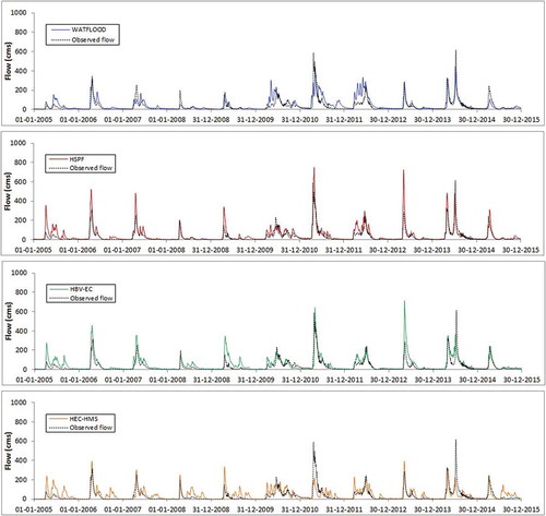
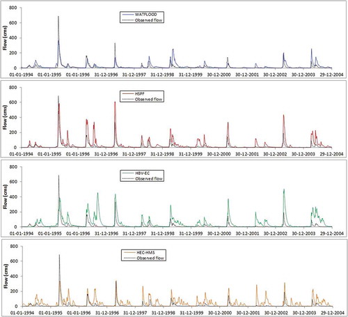
Figure 6. Simulated and observed flows using WATFLOOD, HSPF, HBV-EC and HEC-HMS models for the validation period (1994–2004).

6 Model performance evaluation

Model performance was evaluated based on the most common statistical model comparison tools and other additional parameters, such as model user-friendliness in operational forecasting and required computing time. There are several statistical model performance evaluation criteria employed for model optimization and for comparison of the accuracy of different models (Gupta et al. 1998, Hall 2001, Krause et al. 2005, MacLean 2005, Moriasi et al. 2007, Golmohammadi et al. 2014, Amirhossien et al. 2015, Bhuiyan et al. 2017). In this study, the Nash-Sutcliffe efficiency criterion (NSE; Nash and Sutcliffe 1970), the correlation coefficient (r), root mean squared error (RMSE), mean absolute relative error (MARE) and deviation of runoff volume (D_v) were selected.

The NSE criterion is a measure of statistical association, which indicates the percentage of the observed variance that is explained by the predicted data. It gives more emphasis on extreme events than on average flows. Generally, the NSE ranges from –∞ to 1, with a value of 1 indicating a perfect match of modelled flow rates to the observed data. An efficiency of 0 indicates that the model predictions are as accurate as the mean of the observed data, whereas efficiency less than zero occurs when the observed mean is a better predictor than the model (MacLean 2005, Golmohammadi et al. 2014).

The RMSE measures the model performance with respect to high flow rates, and is very sensitive to outliers (extreme errors). The lower the RMSE value, the better the model performance. The correlation coefficient (r) provides information for linear dependence between observations and corresponding estimates with a value of 1 indicating perfect fit. If a model consistently over- or under-predicts observed values, this can result in a high correlation coefficient, which is misleading. Therefore, it is not necessarily in agreement with other performance criteria such as the RMSE.

The MARE calculates the error as a percentage of the measured value. The optimal value of MARE is zero, with low-magnitude values indicating better model performance. The limitation of MARE is that a small deviation in error can result in large changes in MARE, when calculating with small denominators. Few outliers can dominate the MARE. The MARE not only gives the average performance index in terms of predicting flow rates but also the distribution of the prediction errors (Wieprecht et al. 2013).

The deviation of runoff volume (D_v), also known as the percentage bias, emphasizes volume conservation and is not sensitive to errors in streamflow timing, and smaller values show better model performance (Gupta et al. 1998, MacLean 2005).

The equations for the performance criteria used in this study are given in the Appendix.

6.1 Model performance analysis

Table 5 summarizes the comparison of the statistical model performance criteria NSE, r, RMSE, MARE and D_v for a runoff simulation for the calibration and validation datasets. As can be seen from Table 5, the WATFLOOD model and the HSPF model have comparable results in the calibration period. The WATFLOOD model was the best performing model for the verification period followed by the HSPF model.

Table 5. Comparison of the performance of various hydrological models in simulating runoff in the Shellmouth basin. NSE: Nash-Sutcliffe efficiency criterion; r: correlation coefficient; RMSE: root mean square error; MARE: mean absolute relative error; D_v: deviation of runoff volume (underlined bold indicates the best model performance and bold indicates the second best model performance).

Model	Calibration data					Validation data
	NSE	r	RMSE	MARE	Dv	NSE	r	RMSE	MARE	Dv
			(m^3s^−1)	(%)	(%)			(m^3s^−1)	(%)	(%)
WATFLOOD	0.49	0.77	44.1	184.8	31.4	0.48	0.74	30.1	198.3	53.7
HSPF	0.44	0.85	46.3	128.0	33.8	−0.63	0.81	53.4	211.1	156.3
HBV-EC	0.37	0.82	49.2	185.3	48.6	−1.96	0.62	72.0	500.1	250.5
HEC-HMS	0.39	0.69	48.4	231.5	29.5	−0.40	0.60	49.5	587.9	164.0

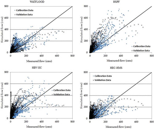
Scatter plots of measured vs simulated flow rates for each model for both calibration and verification periods are shown in Figure 7. As can be seen from Figures 5, 6 and 7, the WATFLOOD model generally performed well for low- and medium-range flows and underestimated higher flows for both calibration and verification periods. The HSPF and HBV-EC models performed well for most flows in the calibration periods, except for showing some inconsistencies at high flows. The HSPF and HBV-EC models overestimated most flows in the validation period. The HEC-HMS model performed reasonably well for low- to medium-range flows in the calibration period and significantly underestimated high flows in both calibration and validation periods. The HEC-HMS model overestimated low- to medium-range flows in the validation period. In general, the HSPF and HBV-EC model performance was good for the calibration period but simulated higher than observed flows for the validation period. The WATFLOOD and HEC-HMS models performed well for low- to medium-range flows, but under-simulated higher flows for both the calibration and validation periods.

Figure 7. Scatter plots of measured vs computed flows using WATFLOOD, HSPF, HBV-EC and HEC-HMS models for the calibration and validation datasets.

6.2 Spring runoff simulation

Often, rivers and streams in the Prairie watershed are characterized by a heavy spring runoff due to snowmelt and spring rain, and have relatively low flows during the summer and winter periods. This is typically true and important for the Shellmouth basin because the Shellmouth Reservoir is intended to store spring runoff and release it whenever it is needed for flood mitigation, water supply or irrigation purposes. Therefore, the performance of the hydrological models for only the spring runoff period is as important as it is for the annual runoff simulation. This analysis is important because a model could perform well for the spring runoff and may not perform well for the winter and summer periods when the flow is low. Therefore, the performance of the hydrological models was evaluated on the accuracy of simulating and forecasting the spring runoff during the period 1 March–25 June, as this is the most important period in terms of runoff contribution to the basin. It has to be noted that the original model parameters were used for this analysis, and model calibration and verification were not done specifically for the spring months.

The summary of statistical model performance criteria for runoff during the spring runoff period is presented in Table 6. As can be seen from Table 6, the HEC-HMS model ranked the best for the spring runoff calibration period, followed by the HSPF model. Considering the validation period, the WATFLOOD model performed best, followed by the HSPF model.

Table 6. Comparison of the performance of the hydrological models in simulating runoff in the Shellmouth basin for the spring runoff period (underlined bold indicates the best model performance and bold indicates the second best model performance).

Model	Calibration data					Validation data
	NSE	r	RMSE	MARE	Dv	NSE	r	RMSE	MARE	Dv
			(m^3 s^−1)	(%)	(%)			(m^3 s^−1)	(%)	(%)
WATFLOOD	0.30	0.68	68.6	89.0	18.2	0.49	0.72	47.4	121.4	20.9
HSPF	0.22	0.85	72.5	76.3	43.3	−0.50	0.80	80.8	195.7	129.5
HBV-EC	0.14	0.82	75.9	111.8	60.0	−1.14	0.64	96.6	369.7	174.2
HEC-HMS	0.45	0.72	60.8	88.0	6.4	0.20	0.66	59.2	224.9	65.7

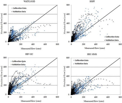
Figure 8 shows scatter plots of measured vs computed flow rates for the spring runoff period (1 March–25 June) for the calibration and validation periods. As can be seen from the scatter plots, performances for the spring period are not significantly different from those of all the flows.

Figure 8. Scatter plots of measured vs computed flows using WATFLOOD, HSPF, HBV-EC and HEC-HMS models for the calibration and validation datasets during the spring runoff period.

7 Operational runoff forecasting in 2016 and 2017

The calibrated and verified models were used for operational flood forecasting of the 2016 and 2017 runoff using real-time hydro-meteorological data.

7.1 Model performance analysis in operational forecasting

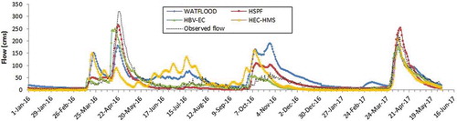
The results of the simulations and the observed inflows into the Shellmouth Reservoir are shown in Figure 9. As can be seen on Figure 9, the HEC-HMS and WATFLOOD models showed a significant early melt in 2016, followed by a smaller melt in April, which is contrary to what was observed. The HEC-HMS and WATFLOOD models also significantly over-predicted runoff for the summer and winter periods of 2016. In contrast, both the HBV-EC and the HSPF models simulated the observed spring runoff reasonably well for 2016 in peak flow, timing and volume of runoff. The HBV-EC and HSPF models also performed reasonably well for the summer and winter periods. All models performed reasonably well in forecasting peak flow, timing and volume of runoff for the 2017 spring runoff period.

Figure 9. Simulated and observed flows using WATFLOOD, HSPF, HBV-EC and HEC-HMS models for operational forecasting in 2016 and 2017.

The statistical model performance evaluation criteria for the 2016–2017 runoff season for all models are summarized in Table 7. As can be seen from Table 7, the HSPF model has the best performance, followed by the HBV-EC model.

Table 7. Comparison of the performance of the different models for operational flood forecasting in 2016 and 2017 (underlined bold indicates the best model performance and bold indicates the second best model performance).

Model	NSE	r	RMSE	MARE	Dv
			(m^3s^−1)	(%)	(%)
WATFLOOD	0.30	0.65	44.1	135.4	40.6
HSPF	0.83	0.91	21.9	45.0	–7.5
HBV-EC	0.80	0.90	23.4	42.3	–14.7
HEC-HMS	0.01	0.42	52.1	155.9	–0.7

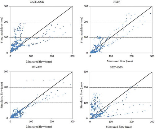
Scatter plots of measured vs computed flow rates for the models for forecasting runoff in the 2016–2017 runoff seasons are presented in Figure 10. As can be seen in Figure 10, the WATFLOOD and HEC-HMS models over-predicted flows for low- to medium-range flows and under-predicted for higher flows, whereas the HSPF and HBV-EC models predicted reasonably well for all ranges of flows.

Figure 10. Scatter plots of measured vs computed flows using WATFLOOD, HSPF, HBV-EC and HEC-HMS models for operational forecasting in 2016 and 2017.

7.2 Computation time, cost and user-friendliness

Another important consideration in model performance for operational forecasting is its computation time, input data requirement and user-friendliness to run the models and obtain the results in a very short time. A short-term (10-day) deterministic forecast and a long-term (30–90 days) ensemble streamflow forecasting methodology is being used at the Manitoba Hydrologic Forecast Centre (HFC) for operational forecasting. Therefore, the model simulation time, input data requirement and user-friendliness were evaluated based on the operational forecasting requirement at the HFC. It is also important to mention that a number of data pre-processing and post-processing tools were developed at the HFC for most models, to improve the efficiency of the model performance. Our analysis, with all these existing internal tools, suggests that, even though there is a slight variance in the computation time, all models are very much comparable in the amount of time they require for simulating the forecasted flows. Once the input data are pre-processed with the tools available to the HFC, there is no significant time difference between the models for simulating flows, as long as they all run on the same powerful computers. In the absence of the data internal tools, the HEC-HMS and the HBV-EC models perform better due to their user-friendliness and smaller input data requirements for model forcing.

In contrast, we found a significant difference in the user-friendliness, or the existence of a graphical user interface (GUI) for the models. The HBV-EC and HEC-HMS models have a very good, user-friendly GUI, making operational forecasting, data input–output and visualization, and model forcing very simple and easy. The HSPF model has a good GUI as well (given through the BASIN software), but its design was focused mainly on United States watersheds. Therefore, the HSPF model requires considerable data processing to be used in Canadian watersheds. The WATFLOOD model does not have a GUI, though it has Green Kenue software to assist in pre- and post-processing.

8 Discussion and conclusions

From the model results, it can be concluded that all four models (WATFLOOD, HBV-EC, HSPF and HEC-HMS) are capable of simulating flows fairly accurately and can be used for operational flood forecasting. The HSPF and WATFLOOD models performed better in calibration and verification for the entire calibration and validation periods. However, the HEC-HMS and HSPF models performed better in simulating spring runoff. Interestingly, the HBV-EC and HSPF models performed better in forecasting the runoff for the 2016–2017 periods. The WATFLOOD and HEC-HMS models generally performed better for low flows, but were not particularly good in simulating high flows, whereas the HSPF and HBV-EC models performed better in simulating high flows, but over-predicted low flows in most cases.

Our conclusion is that a single hydrological model could not be considered adequate to simulate the runoff process in the basin accurately. Therefore it is recommended to use multiple models and implement probabilistic ensemble prediction systems for operational forecasting. This is due to the complex weather patterns in the Prairie region and also the complex landscape, with many small potholes that store water and prevent flow contributing to the main stream. In addition, the contributing areas continually change within a runoff season depending on the wetness of the basin. Each model reacts differently to this hydrological phenomenon (fill and spill of the potholes) and the results of the model performances have shown this hydrological complexity. Furthermore, there is an inherent model uncertainty in developing a model for predicting future hydrological responses owing to various factors, such as limitations in the calibration of the hydrological model, a lack of understanding of the physical basin parameters, and lack of good data on the key drivers such as precipitation, as well as lack of accurate data that represent the current status of the land-use changes. Having multiple hydrological models and using them on a continuous simulation basis, coupled with the forecaster’s knowledge of the hydrology of the basin, would provide a reasonably accurate flow forecast. The findings of this study should only be used in the context of operational flow forecasting in the Prairie watershed. Generalization of the findings of this study for use in other non-Prairie watersheds may not be accurate.

Disclosure statement

No potential conflict of interest was reported by the authors.

Appendix

The performance criteria are computed as follows:

Nash-Sutcliffe efficiency:

(A1)

Correlation coefficient:

(A2)

Root mean square error:

(A3)

Mean absolute relative error:

(A4)

Relative error:

(A5)

Deviation of runoff volume:

(A6)

where RE is the relative error in prediction expressed as a percentage, O_i is the observed streamflow for the ith time step, S_i is the simulated streamflow for the ith observation, is the mean simulated value, is the mean observed value, and N is the total number of observations.

References

- Amirhossien, F., et al., 2015. A comparison of ANN and HSPF models for runoff simulation in Balkhichai River Watershed, Iran. American Journal of Climate Change, 4 (3), 203–279. doi:10.4236/ajcc.2015.43016
- Bergström, S., 1995. The HBV model. In: V.P. Singh, ed. Computer models of watershed hydrology. Highland Ranch, CO: Water Resources Publications, 443–476.
- Bhuiyan, H.A., et al., 2017. Application of HEC-HMS in a cold region watershed and use of RADARSAT-2 soil moisture in initializing the model. Hydrology, 4 (1), 9. doi:10.3390/hydrology4010009
- Bicknell, B.R., et al., 2005. HSPF version 12.2 user’s manual. Mountain View, California: AQUA TERRA Consultants.
- Burn, D. and Whitfield, P., 2016. Changes in floods and flood regimes in Canada. Canadian Water Resources Journal, 41 (1–2), 139–150. doi:10.1080/07011784.2015.1026844
- Buttle, J.M., et al. 2016. Flood processes in Canada: regional and special aspects. Canadian Water Resources Journal, 41 (1–2), 7–30. doi:10.1080/07011784.2015.1131629
- Canadian Hydraulics Centre, 2010. Green kenue reference manual. Ottawa, Ontario: National Research Council.
- Carsell, K.M., Pingel, N.D., and Ford, D.T., 2004. Quantifying the benefit of a flood warning system. Natural Hazards Review, 5 (3), 131–140. doi:10.1061/(ASCE)1527-6988(2004)5:3(131)
- Chu, X. and Steinman, A., 2009. Event and continuous hydrologic modeling with HEC-HMS. Journal of Irrigation and Drainage Engineering-ASCE, 135 (1), 119–124. doi:10.1061/(ASCE)0733-9437(2009)135:1(119)
- Cranmer, A.J., Kouwen, N., and Mousavi, S.F., 2001. Proving WATFLOOD: modelling the nonlinearities of hydrologic response to storm intensities. Canadian Journal of Civil Engineering, 28 (5), 837–855. doi:10.1139/l01-049
- Crawford, N.H. and Linsley, R.K., 1966. Digital simulation in hydrology: stanford watershed model 4. California: Departrment of Civil Engineering, Stanford University. Technical Rep. 39.
- Cunderlik, J.M. and Simonovic, S.P., 2004. Calibration, verification and sensitivity analysis of the HEC-HMS hydrologic model. London, Ontario: Department of Civil and Environmental Engineering, The University of Western Ontario. Water Resources Research Report no. 048.
- Donigian Jr., A.S., et al., 1984. Application guide for hydrological simulation program: FORTRAN (HSPF). Washington, DC: US Environmental Protection Agency, EPA.
- Dumanski, S., Pomeroy, J.W., and Westbrook, C.J., 2015. Hydrological regime changes in a Canadian Prairie basin. Hydrological Processes, 29 (18), 3893–3904. doi:10.1002/hyp.v29.18
- Environment Agency, 2003. Flood Warning Investment Strategy Appraisal Report 2003/04 to 20012/13. National Flood Warning Centre, Frimley.
- Fang, X., et al., 2007. A review of Canadian Prairie hydrology: principles, modelling and response to land use and drainage change. Saskatoon: Centre for Hydrology, University of Saskatchewan.
- Feldman, A.D., 2000. Hydrologic modeling system HEC-HMS: technical reference manual. Davis, CA: US Army Corps of Engineers, Hydrologic Engineering Center.
- Flood Recovery Task Force, 2013. Southern Alberta 2013 floods: the provincial recovery framework. Edmonton: Government of Alberta.
- Godwin, R. and Martin, F. 1975. Calculation of gross and effective drainage areas for the Prairie. Proceedings of the Canadian Hydrology Symposium. Winnipeg, Manitoba, pp 219–223.
- Golmohammadi, G., et al., 2014. Evaluating three hydrological distributed watershed models: MIKE-SHE, APEX, SWAT. Hydrology, 1 (1), 20–39. doi:10.3390/hydrology1010020
- Granger, R.G., Gray, D.M., and Dyck, G.E., 1984. Snowmelt infiltration to frozen prairie soils. Canadian Journal of Earth Science, 21 (6), 669–677. doi:10.1139/e84-073
- Gray, D.M., 1970. Handbook on the principles of hydrology. Port Washington, New York: Water Information Center Inc.
- Gray, D.M. and Landine, P.G., 1988. An energy-budget snowmelt model for the Canadian Prairies. Canadian Journal of Earth Science, 25 (8), 1292–1303. doi:10.1139/e88-124
- Gray, D.M., et al., 2001. Estimating areal snowmelt infiltration into frozen soils. Hydrological Processes, 15 (16), 3095–3111. doi:10.1002/(ISSN)1099-1085
- Grillakis, M.G., Tsanis, I.K., and Koutroulis, A.G., 2010. Application of the HBV hydrological model in a flash flood case in Slovenia. Natural Hazards and Earth System Sciences, 10 (12), 2713–2715. doi:10.5194/nhess-10-2713-2010
- Gupta, H.V., Sorooshian, S., and Yapo, P.O., 1998. Toward improved calibration of hydrologic models: multiple and noncommensurable measures of information. Water Resour Research, 34 (4), 751–763. doi:10.1029/97WR03495
- Hall, M.J., 2001. How well does your model fit the data? Journal of Hydroinformatics, 3 (1), 49–55.
- Hamilton, A.S., Hutchinson, D.G., and Moore, R.D., 2000. Estimating winter streamflow using conceptual streamflow model. Journal of Cold Regions Engineering, 14 (4), 158–175. doi:10.1061/(ASCE)0887-381X(2000)14:4(158)
- Hayashi, M., van der Kamp, G., and Schmidt, R., 2003. Focused infiltration of snowmelt water in partially frozen soil under small depressions. Journal of Hydrology, 270 (3–4), 214–229. doi:10.1016/S0022-1694(02)00287-1
- Hundecha, Y. and Bárdossy, A., 2004. Modeling of the effect of land use changes on the runoff generation of a river basin through parameter regionalization of a watershed model. Journal of Hydrology, 292 (1–4), 281–295. doi:10.1016/j.jhydrol.2004.01.002
- Jakob, M. and Church, M., 2011. The trouble with floods. Canadian Water Resources Journal, 36 (4), 287–292. doi:10.4296/cwrj3604928
- Jenkinson, R.W., 2009. Surface water quality modelling considering Riparian wetlands. Thesis (PhD). University of Waterloo.
- Jost, G., et al., 2012. Quantifying the contribution of glacier runoff to streamflow in the upper Columbia river basin, Canada. Hydrology and Earth Systems. Sciences, 16 (3), 849–860. doi:10.5194/hess-16-849-2012
- Kouwen, N., 1973. Watershed modeling using a square grid technique. Proceedings of First Canadian Hydraulics Conference, CSCE Edmonton, pp. 418–434.
- Kouwen, N., 1988. WATFLOOD: a micro-computer based flood forecasting system based on real-time weather radar. Canadian Water Resources Journal, 13 (1), 62–77. doi:10.4296/cwrj1301062
- Kouwen, N., 2016. WATFLOOD™/CHARM Canadian hydrological and routing model. User’s manual. Waterloo: University of Waterloo.
- Kouwen, N., et al., 1993. Grouped response units for distributed hydrologic modeling. Journal of Water Resources Planning and Management-ASCE, 119 (3), 289–305. doi:10.1061/(ASCE)0733-9496(1993)119:3(289)
- Krause, P., Boyle, D.P., and Bäse, F., 2005. Comparison of different efficiency criteria for hydrological model assessment. Advances in Geoscience, 5, 89–97. doi:10.5194/adgeo-5-89-2005
- Lindström, G., et al., 1997. Development and test of the distributed HBV-96 hydrological model. Journal of Hydrology, 201 (1–4), 272–288. doi:10.1016/S0022-1694(97)00041-3
- MacLean, A., 2005. Statistical Evaluation of WATFLOOD. Waterloo: Department of Civil and Environmental Engineering, University of Waterloo.
- Mahat, V. and Anderson, A., 2013. Impacts of climate and catastrophic forest changes on streamflow and water balance in a mountainous headwater stream in Southern Alberta. Hydrology and Earth Systems. Sciences, 17, 4941–4956. doi:10.5194/hess-17-4941-2013
- Manitoba Infrastructure and Transportation, 2013. Manitoba 2011 Flood Review Task Force Report. Winnipeg: Report to the Minister of Infrastructure and Transportation.
- Moriasi, D.N., et al., 2007. Model evaluation guidelines for systematic quantification of accuracy in watershed simulations. American Society of Agricultural and Biological Engineers, 50 (3), 885–900.
- Mousavi, S.J., et al., 2012. Uncertainty-based automatic calibration of HEC-HMS model using sequential uncertainty fitting approach. Journal of Hydroinformatics, 14 (2), 286–309. doi:10.2166/hydro.2011.071
- Muhammad, A., et al., 2016. Parameter and model structure uncertainty in stream flow simulation of upper Assiniboine river basin through soil water assessment tool (SWAT) and NAM model. Vienna: EGU General Assembly.
- Nash, J.E. and Sutcliffe, J.V., 1970. River flow forecasting through conceptual models part-I: a discussion of principles. Journal of Hydrology, 10 (3), 282–290. doi:10.1016/0022-1694(70)90255-6
- Neff, T.A., 1996. Mesoscale water balance of the boreal forest using operational evapotranspiration approaches in a distributed hydrologic model. Thesis (PhD). University of Waterloo.
- Pappenberger, F., et al., 2015. The monetary benefit of early flood warnings in Europe. Environmental Science and Policy, 51, 278–291. doi:10.1016/j.envsci.2015.04.016
- Parker, D.J., Tunstall, S., and Wilson, T., 2005. Socio-economic benefits of flood forecasting and warning. International conference on innovation advances and implementation of flood forecasting technology, 17-19 October 2005, Tromsø, Norway.
- Penning-Rowsell, E.C., et al., 2000. The benefits of flood warnings: real but elusive, and politically significant. Water and Environment Journal, 14 (1), 7–14. doi:10.1111/wej.2000.14.issue-1
- Philip, J.R., 1954. An infiltration equation with physical significance. Soil Sciences Journal, 77 (2), 153–158. doi:10.1097/00010694-195402000-00009
- Pomeroy, J.W., De Boer, D., and Martz, L.W., 2005. Hydrology and Water Resources of Saskatchewan, Center for Hydrology Report #1. Saskatoon: Centre for Hydrology, University of Saskatchewan.
- Pomeroy, J.W., et al., 2007. The cold regions hydrological model: a platform for basing process representation and model structure on physical evidence. Hydrological Processes, 21 (19), 2650–2667. doi:10.1002/(ISSN)1099-1085
- Pomeroy, J.W., et al., 1998. An evaluation of snow accumulation and ablation processes for land surface modelling. Hydrological Processes, 12 (15), 2339–2367. doi:10.1002/(ISSN)1099-1085
- Pomeroy, J.W., Stewart, R.E., and Whitfield, P.H., 2016. The 2013 flood event in the South Saskatchewan and Elk River basins: causes, assessment and damages. Canadian Water Resources Journal, 41 (1–2), 105–117. doi:10.1080/07011784.2015.1089190
- Upper Assiniboine River Basin Study, 2000. Study Report Prepared at the Conclusion of the Upper Assiniboine River Basin Study Agreement Signed in October 1996 by the Governments of Saskatchewan, Manitoba and Canada.
- USACE-HEC, 2015. Hydrologic modeling system (HEC-HMS), application guide, version 4.0. Davis, CA: US Army Corps of Engineers, Hydrologic Engineering Center.
- USACE-HEC, 2016. Hydrologic modeling system HEC-HMS, user’s manual, version 4.2. Davis, CA: US Army Corps of Engineers, Hydrologic Engineering Center.
- USGS, 1997. Water resources applications software, summary of hydrological simulation program—fortran (HSPF). Reston, VA: US Geological Survey.
- WaterSMART, A., 2013. The 2013 great Alberta flood: actions to mitigate, manage and control future floods. Calgary: Alberta WaterSMART, Water Management Solutions.
- Wieprecht, S., Tolossa, H.G., and Yang, C.T., 2013. A neuro-fuzzy-based modelling approach for sediment transport computation. Hydrological Sciences Journal, 58 (3), 587–599. doi:10.1080/02626667.2012.755264
- Zegre, N.P., 2008. Local and downstream effects of contemporary forest harvesting on streamflow and sediment yield. Dissertation (PhD). Oregon State University.
- Zhang, X. and Lindström, G., 1997. Development of an automatic calibration scheme for the HBV hydrological model. Hydrological Processes, 11 (12), 1671–1682. doi:10.1002/(ISSN)1099-1085
- Zhao, L. and Gray, D.M., 1997. A parametric expression for estimating infiltration into frozen soils. Hydrological Processes, 11 (13), 1761–1775. doi:10.1002/(ISSN)1099-1085