Suspended sediment yield estimation using genetic algorithm-based artificial intelligence models: case study of Mahanadi River, India

ABSTRACT

The estimation of sediment yield is important in design, planning and management of river systems. Unfortunately, its accurate estimation using traditional methods is difficult as it involves various complex processes and variables. This investigation deals with a hybrid approach which comprises genetic algorithm-based artificial intelligence (GA-AI) models for the prediction of sediment yield in the Mahanadi River basin, India. Artificial neural network (ANN) and support vector machine (SVM) models are developed for sediment yield prediction, where all parameters associated with the models are optimized using genetic algorithms simultaneously. Water discharge, rainfall and temperature are used as input to develop the GA-AI models. The performance of the GA-AI models is compared to that of traditional AI models (ANN and SVM), multiple linear regression (MLR) and sediment rating curve (SRC) method for evaluating the predictive capability of the models. The results suggest that GA-AI models exhibit better performance than other models.

KEYWORDS:

• genetic algorithm
• artificial intelligence
• suspended sediment yield
• water discharge
• Mahanadi River

Editor M.C. Acreman Associate editor A. Jain

1 Introduction

The volume of sediment transported in a river provides important information about its morphodynamics, the hydrology of its drainage basin, and the erosion and sediment delivery processes operating within that basin (Walling 2009). The functioning of a river system is also significantly controlled by the magnitudes of the sediment loads transported by the rivers, as sediment fluxes play a pivotal role in channel morphology, delta development, geochemical cycling of elements, water quality, aquatic ecosystems and habitats supported by the river (Cigizoglu 2004, Walling 2009, Kisi and Shiri 2012). Rivers are very important for the growth of human civilization and therefore have their own socio-economic dimension. Also, the sediment loads of rivers can influence the use of a river for water supply, channel navigation, natural and wildlife habitat, and fishing. High sediment concentrations in rivers can, in particular, be responsible for major problems of water resource development through reservoir sedimentation and the siltation of water diversion and irrigation schemes, as well as increasing the cost of treating water abstracted from a river (Walling 2009). High sediment inputs to lakes and coastal seas can result in sedimentation and changes in nutrient cycling. In addition, high sedimentation in the downstream part of a river leads to severe flooding during heavy rain. Hence, it is essential to estimate the quantity of sediment flowing in a river (ZICL 2014, Kafle et al. 2015). According to the current best global estimate, 18 × 10⁹ tonnes(t)/year of riverine sediment flux is transferred to the ocean (Milliman and Syvitski 1992). The rivers that flow through the Indian sub-continent have transferred 15–20% of the global sediment to the ocean (Gupta et al. 2012). The quantitative estimation of sediment loads in a river is either labour intensive by manual operation or economically expensive by automatic sampling devices.

The determination of sediment yield using traditional methods is not very accurate due to the involvement of various complex processes. A traditional multiple linear regression (MLR) mathematical model has been used for sediment yield prediction (Zhu et al. 2007, Rajaee et al. 2009). The MLR models have the ability to capture any linear relationship; however, they fail to model the presence of nonlinearity in hydroclimatic data. The first nonlinear model used for sediment discharge estimation was the sediment rating curve (SRC) model (Sandy 1990, Jain 2001). The SRC model uses a power law function in order to capture nonlinearity. The main limitation of the SRC model is that it can only consider a single independent variable (quantity of discharge); however, several researchers have demonstrated that other variables, such as rainfall and temperature, also play an important role in sediment loads (Lenzi and Marchi 2000, Khoi and Suetsugi 2014, Buendia et al. 2016). Moreover, the SRC can only model the sediment data reasonably well if the nonlinearity follows a specific function, i.e. the power law. In order to overcome these limitations, in the past two decades, different artificial intelligence (AI) models including the ANN and SVM have seen increasing popularity for the simulation of hydrological processes (Dibike et al. 2001, Wang et al. 2008, Singh and Panda 2011). The main advantage of AI models is that they can handle both linear and nonlinear dependency with multiple variables. Numerous ANN and SVM models have been successfully applied by various researchers for the estimation of sediment concentration and sediment load (Rajaee et al. 2009, Haji et al. 2014, Sharma et al. 2015). It has also been observed that AI models provide better results than traditional methods, such as MLR and the SRC (Zhu et al. 2007, Rajaee et al. 2009, Haji et al. 2014, Sharma et al. 2015, Ahmadi and Rodehutscord 2017, Yadav et al. 2017). Both ANN and SVM are data-driven approaches, where a set of training data is required to develop the model. Fundamentally, these two algorithms are very different. Neural networks work iteratively by minimizing errors (Singh and Panda 2011), whereas the SVM works on the basis of the quadratic optimization principle (Vapnik 1995). Although the SVM relies on structural risk minimization in order to reach the global optimum solution, researchers extensively show that the neural network performs equally well in terms of solving complex nonlinear regression problems (Sharma et al. 2015, Ahmadi and Rodehutscord 2017, Patel et al. 2017).

The main limitation of the ANN is represented by problems of over- and underfitting (Bishop 1998). Underfitting leads to poor network performance with a training dataset, whereas overfitting leads to a poor generalization of the model. This means that the model may work in a good way with training data, but perform poorly in predicting testing data for the overfitting model, and the reverse for the underfitting model. Fitting problems are normally caused by poor selection of the neural network parameters, such as the combination coefficient, and network topology, such as the hidden node size, i.e. nodes in hidden layers, number of hidden layers, initial weights, etc. Although the SVM provides a global optimum solution, inaccurate selection of kernel function and SVM hyper-parameters, such as regularization parameter (C), may lead to a poor generalized model (Chatterjee and Bandopadhyay 2011, Zhang et al. 2015). Traditionally, trial-and-error methods are followed in ANN models to select the learning parameters and network topology (number of input and hidden nodes), and in SVM models to select kernel functions and hyper-parameters. However, trial-and-error methods may not provide the optimum selection of these parameters, and they are computationally expensive. Therefore, the selection of these parameters in the ANN and SVM models is an essential task in developing robust AI models.

To overcome the limitations of parameter selection for ANN and SVM models, researchers have been using the GA approach over the past decade (Castillo et al. 2000, Wang et al. 2008, Chatterjee and Bandopadhyay 2011, Su et al. 2013, Adib and Mahmoodi 2017). The GA produces a set of possible solution points during an adaptive and dynamic system structure evolution (Altunkaynak 2008). The main advantage of the GA for ANN and SVM modelling is that the GA has the ability both to prevent the ANN from becoming trapped in a local minimum zone and to select the optimal parameters for the SVM model (Gupta and Sexton 1999, Tahmasebi and Hezarkhani 2009, Li and Kong 2014, Zhang et al. 2015). Recently, in hydrological studies and other fields, it has been shown that GA-based ANN (GA-ANN) and GA-based SVM (GA-SVM) models provided better prediction results than traditional neural network and SVM models (Chau et al. 2005, Chatterjee and Bandopadhyay 2007, 2011, 2012, Chiu and Chen 2009, Su et al. 2013).

The GA-ANN and GA-SVM models have been successfully applied for the prediction and forecasting of streamflow, flood, bedload transport, reservoir storage, rainfall and runoff (Chau et al. 2005, Parasuraman and Elshorbagy 2007, Wang et al. 2008, Sedki et al. 2009, Asadi et al. 2013, Su et al. 2013). Sirdari et al. (2015) used genetic programming and ANN-based models to estimate bedload transport in the Kurau River, Malaysia. The GA-based model has been applied recently for the prediction of suspended sediments in the Karun and Marun rivers of Iran (Adib and Jahanbakhshan 2013, Adib and Mahmoodi 2017), the Lower Mississippi River, USA (Altunkaynak 2009) and the Rio Valenciano and the Quebrada Blanca station, Puerto Rico (Kisi and Guven 2010). Su et al. (2013) developed the GA-SVM model for the prediction of the monthly reservoir storage of the Miyun Reservoir in North China and found that the GA-SVM model showed the best prediction capability compared to other hybrid optimization algorithms.

Research on the optimization of the ANN and SVM training parameters has been done widely, including the application of the GA for the optimization of the input parameters, connection and biased weights, and number of neurons of the hidden layer in the ANN (Fatemi et al. 2003, Jain and Srinivasulu 2004, Chatterjee and Bandopadhyay 2007, Adib and Jahanbakhshan 2013, Adib and Mahmoodi 2017). In all cases, the GA was used in order to optimize a single parameter at a time.

Research on the optimization of multiple parameters of the ANN and SVM using the GA to optimize all parameters at the same time has been conducted widely (Admuthe et al. 2009, Chatterjee and Bandopadhyay 2011, Correa et al. 2011, Li and Kong 2014, Zhang et al. 2015). The simultaneous optimization of multiple parameters of the ANN using the GA outperforms the optimization of a single parameter because the simultaneous optimization of all parameters may lead to global optimization (Maniezzo 1994, Kim and Ahn 2012). Simultaneous multiple parameter optimization is applied to overcome the limitations of the trial-and-error method by reducing computational time and providing an accurate result (Admuthe et al. 2009, Chatterjee and Bandopadhyay 2012, Kim and Ahn 2012). Similarly, the simultaneous optimization of features and SVM parameters using the GA has reduced the computational time and provided more accurate results when searching for the optimal parameter (Zhao et al. 2011, Zhang et al. 2015).

Although the simultaneous optimization of multiple training parameters and the architecture of the network for AI models has been successfully applied in other disciplines (Chatterjee and Bandopadhyay 2011, 2012, Correa et al. 2011, Zhang et al. 2015), to the best of the knowledge of the authors, there is no such study available for sediment yield estimation in river basins. In this study, AI models (ANN and SVM) were developed, in which all the parameters of the ANN (input variables, hidden layer neurons, combination coefficients, transfer functions and network weights) and of the SVM (input variables, cost parameters, basis functions, parameters associated with basis functions) were optimized simultaneously, and then applied for sediment yield estimation.

The Mahanadi River is the second largest Indian peninsular river in terms of water potential and flood-producing capacity (India-WRIS 2015). Various ANN and mathematical models have been successfully used for the estimation and forecasting of streamflow, rainfall and runoff, and flooding in the Mahanadi River basin (Pramanik and Panda 2009, Kar et al. 2010, Meher and Jha 2013, Meher 2014, Khan et al. 2016). For example, Kashid et al. (2010) used the GA for the prediction of streamflow in the Mahanadi River basin. However, very few works have been done on sediment yield prediction in the Mahanadi River. Ghose et al. (2012) developed ANN and GA models at the Basantpur gauging station, located in the upper part of the Mahanadi River, to identify the optimum water discharge and temperature for predicting the minimum sediment load. Moreover, a global sediment yield estimation using GA-ANN has been carried out in various rivers having small catchment areas ranging from 8.63 to 6423 km², as well as in the Lower Mississippi and Karun rivers, which have catchment areas of 57 730 and 66 930 km², respectively. In this study, GA-ANN and GA-SVM models were developed in order to estimate the sediment yield in the downstream Tikarapara station of the Mahanadi River, which has a catchment area of about 124 450 km². In addition, the performance of the GA-ANN and GA-SVM models was compared to the traditional ANN, SVM, MLR and SRC models to evaluate the predictive capability of various models.

2 Methodology

2.1 Genetic algorithm-based artificial neural network (GA-ANN)

The customized code for this model was developed in Matlab 2012a (Mathwork 2012) software, and the normalized data were used for neural network parameter selection. The ANN is a flexible and well-established mathematical tool, which can be used to solve many complex nonlinear problems by correlating the input and output datasets to obtain approximate results. It works on the basis of the concept of the biological brain and its associated nervous system (Haghizade et al. 2010).

In this study, a multilayer perceptron (MLP) feedforward neural network with a fast convergence training algorithm, i.e. the Levenberg-Marquardt (LM) back-propagation algorithm, was used to predict the suspended sediment yield (Cobaner et al. 2009, Pramanik and Panda 2009). The main advantage of this algorithm is that it is robust and the convergence is very fast (Demuth and Beale 1998). This algorithm is used for updating the connection and bias weights of the network. The feedforward back-propagation Levenberg-Marquardt (FFBP-LM) algorithm was used to develop the robust MLP neural network model due to its fast response. Thus, it is a first choice to supervise the algorithm, although it requires more memory (Adeloye and Munari 2006).

The feedforward network contains one input layer, one hidden layer and one output layer. Each layer consists of a specific number of neurons and bias weights with activation functions. The neurons of one layer are connected to those of another layer through weighted interconnected links and these weights contain extremely important information in the ANN. Many studies have demonstrated that a single hidden layer is adequate to approximate to any complex nonlinear function and also to reduce structure complexity (Hornik et al. 1989, Tang et al. 1991).

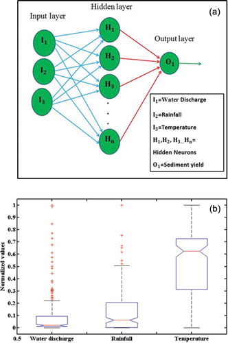
In the MLP, each neuron in a layer transfers the sum of weighted input parameters into an activation level through the activation function to the next layer, and this function must be monotonically increasing and differentiable (Cobaner et al. 2009, Boukhrissa et al. 2013). The diagram of the MLP model for suspended sediment yield prediction is shown in Figure 1(a).

Figure 1. (a) Artificial neural network architecture for three-layer feedforward network. (b) ANOVA test result of the input data. I: input neurons; H: hidden neurons; O: output neurons. The arrows represent the connection weights between the layers.

To control the training of the neural network, a random initialization of weights was applied. The neurons and input parameters of the network were changed to allow us to understand the effect of the input parameters on the sediment yield estimation. The weight update rule of the FFBP-LM optimization algorithm is derived by the steepest descent and Newton’s method (Hagan and Menhaj 1994) and expressed as:

(1)

where J is the Jacobian matrix, I is the identity matrix, e is the error vector, k is the iteration number, W is the weight vector, and µ is the non-negative scalar value that affects the learning process of FFBP-LM in the ANN, referred to as the combination coefficient. When µ = 0, the FFBP-LM algorithm is working as Newton’s method, whereas when µ is large, that becomes the gradient descent approach with a small step size (Pramanik and Panda 2009). Therefore, the proper selection of the parameter µ is a crucial task in the LM method; this parameter was selected along with other parameters within the genetic algorithm framework, as discussed later. The error vector e was calculated by considering the difference between the actual output and the predicted output. The error is back-propagated through the network to each neuron, corresponding connection and bias weight. The Jacobian matrix is calculated by taking the partial derivatives of e with respect to all unknown parameters, i.e. weights and bias terms.

The performance of the MLP neural network models depends on many factors including the input parameters, number of nodes in the hidden layer, the activation function used in different layers, and the values of initial weights. The wrong selection of any one of these factors may result in a poor neural network model. In this study, we selected all these factors simultaneously using the genetic algorithm.

The genetic algorithm (GA) is a population-based optimization algorithm based on Darwin’s theory of evolution, which is used for finding the best parameters for the ANN models (Holland, J. 1975). It creates diversity in the population of individuals (chromosomes) of the given problem using various genetic operators such as mutation, selection and cross-over. The GA is a widely applicable optimization algorithm to solve various non-differentiable, discontinuous, stochastic or highly nonlinear problems in a noisy environment (Goldberg 1989, Beyer 2000). In this study, we used the GA in conjunction with the multilayered feedforward ANN having a single hidden layer (hereafter referred to as GA-ANN). The neural network training was done using the LM algorithm, and all parameter selection was made by means of the GA. The parameter selection and ANN training were performed simultaneously in order to yield a more robust solution that has little chance of becoming trapped in the local optimum point.

The GA technique is designed for producing successive populations having various individuals with different types of characteristics. The purpose of using the GA in this study was to select five major parameters for the ANN models, namely inputs, the transfer function, number of neurons in the hidden layer, combination coefficient, and connection and bias weights. All five neural network parameters are encoded to a binary string known as a chromosome. Multiple such chromosomes are randomly initialized and updated iteratively by genetic operations, such as selection, cross-over and mutation, in order to generate improved solutions. Each chromosome has five parts, and each part represents one neural network parameter. The first part of the chromosome represents the input parameters. This part contains a 3-bits binary value. If the bit value is 1, then the concerned input is included in the specified subset; likewise, if the bit value is zero, then the corresponding input is not included in the subset. For example, if the binary code is represented as 101, then input 1 and input 3 will be considered for the neural network model, and input 2 will be excluded. Similarly, the second part of the chromosome represents the transfer function for the hidden and output layers, which were represented by the 3-bits binary number. This part represents the transfer functions for both the hidden layer and the output layer.

In this study, three different transfer functions, i.e. the log-sigmoidal, tan-sigmoidal and linear functions, were tested. There are nine different possible combinations of transfer functions that can be used for the hidden and output layers. However, the linear transfer function in both the hidden and output layers transforms the neural network model into a complete linear model. We excluded that model in the GA-ANN modelling in this study because the multiple linear regression was modelled separately. The third part of the chromosome contains five bits and represents the number of nodes in the hidden layer. During modelling, this binary code is converted to decimals in order to generate hidden node numbers. The maximum number of hidden neurons was restricted to 32, keeping in view the computational time and model complexity. The lower bound of the hidden neurons was also fixed as 1. The 5-bits chromosomes can represent all decimal numbers from 1 to 32. The fourth part of the chromosome represents the combination coefficient (µ) using an 8-bit binary number. The 8-bit binary number can be converted within the range of µ (0.001 to 9 × 10⁹) by means of the normalization process.

The normalization process of µ is conducted using the following normalization equation:

(2)

where a and b are the maximum and minimum values within which µ is to be normalized; here, µ ranges between 0.001 and 9 × 10⁹; therefore, a and b are 0.001 and 9 × 10⁹, respectively; C_norm is the normalized value of C_i, the decimal value of the fourth part of the ith chromosomal 8-bits binary value; and C_max and C_min are the maximum and minimum decimal values of the 8-bits binary number of µ, respectively.

The fifth part of the chromosome represents the connection weights and bias terms of the neural network models. This part has a variable length due to the change in input numbers and number of nodes in the hidden layer. The number of weight and bias terms is fully dependent on the number of input and hidden nodes. If the number of input nodes is m, and number of hidden neurons is n, then the number of weight and bias terms (N) in the single output neural network model can be calculated by:

(3)

Each weight is given by the 8-bit binary number, and the number of bits to represent the connection weights and bias terms is 8 × [n × (m + 1) + (n × 1) + 1]. Therefore, when m = 3 and n = 32, the number of connection weights and biased terms will be 161.

For the selection method, a pair of parent chromosomes was chosen from the initial population for the creation of offspring in successive generations on the basis of better fitted individuals. The chromosome is uniformly initialized. The number of chromosomes in the population, i.e. the population size, was taken as 50 in order to reduce computational time and maintain diversity (Chatterjee and Bandopadhyay 2012). The ANN model was trained for each chromosome using the training data and the fitness value was calculated using the validation data. The fitness function gives a measurement of the success of chromosomes and also estimates the chance of acceptance of chromosomes for the population in successive generations. The individual chromosome with a better fitness function value has a better chance to be selected for the next generation. Based on individual fitness values, some chromosomes are selected by elitism. Cross-over and mutation operations are then performed for the selected chromosomes by the roulette-wheel selection criterion, which is based on the calculated fitness function (Davis 1991).

The roulette-wheel selection method was used for determining the elite members in the population and finally reproduction took place with recombination in order to generate offspring. The number of elites passed to the next generation of the genetic algorithm is 2 (Zanaganeh et al. 2009). The cross-over operation is performed in each generation in order to generate a better solution from the available solutions. New individuals have been found to benefit from the parent fitness through the cross-over operation. This operation is carried out by creating the individuals by interchanging the genetic material of the chromosomes so that they can benefit from their parent’s fitness. The mutation operator is responsible for providing variety in the population. It operates by randomly flipping bits (0–1 or 1–0) of the chromosomes based on the user-selected mutation rate.

The performance of the GA depends on a high probability of the cross-over and a low probability of the mutation (Dejong 1975). In this study, a uniform cross-over with a probability rate of 0.6 was used (Chatterjee and Bandopadhyay 2011). The mutation operation helps the algorithm to escape the solution from local minima. Low constant mutation probability of 0.05 was used in this study (Chatterjee and Bandopadhyay 2011); a small value is usually taken in order to avoid the algorithm going into a random search. The root mean square error (RMSE) of the validation dataset was used as the fitness function for the genetic algorithm of this study. The fitness values of all chromosomes were estimated using the RMSE. After each generation, “bad” chromosomes with a low fitness function value were eliminated in order to maintain a population size of 50. The obtained population of chromosomes after one generation is the starting solution for the next generation. The genetic operation was performed until a stopping criterion such as the maximum generation was reached.

A minimum RMSE of the fitness function or minimum change to the fitness function in various consecutive generations is found. The maximum number of generations used in this study was 100 (Zanaganeh et al. 2009). The best solution value is obtained on the basis of the minimum RMSE of the fitness value after the final generation. The chromosome from the population corresponding to that best solution is the optimal neural network parameters (input variables, transfer functions, number of hidden neurons, µ value, and initial network weights and bias terms) for the ANN model.

2.2 Genetic algorithm-based support vector machine (GA-SVM)

The SVM was originally developed by Vapnik based on the structural risk minimization principle (Vapnik 1995). The desirable property of the SVM is to maximize the margin and thereby improve the generalization ability (Smola 1996, Saunders et al. 1998). It has been used extensively and consistently achieves similar or superior performance compared to other machine learning methods (Heikamp and Bajorath 2014). The main idea of the SVM is to map data points to a high dimension space with a kernel function, and then these data points can be separated by a hyper-plane in that space for a better generalization error of the model (Sharma et al. 2015, Zhang et al. 2015). Although, the SVM was initially developed as a classification tool, it has been successfully used for regression problems. The SVM has been proved to be a novel algorithm with good performance. However, the performance of the SVM model depends highly on the right selection of its parameters. In the SVM, the kernel function provides the opportunity for using a nonlinear function in the input space for varying the linear function in the characteristics space. Similar to other multivariate statistical models, the performance of the SVM regression model depends on the combination of several parameters including the number of input variables in the regression model, regularization parameter C (controls the trade-off between training error and model complexity), parameter ε (controls the width of the ε-insensitive zone), to fit the training data, kernel function (most commonly Gaussian, radial basis function, linear and polynomial are used), and hyper-parameters associated with the kernel function. If C is too large, the model will have a high penalty for non-separable points and may store too many support vectors, resulting in overfitting. If it is too small, the model may have underfitting. The value of ε can affect the number of support vectors used to construct the regression function: the higher the value of ε, the fewer the support vectors to be selected, while higher ε values result in more flat estimates. Both C and ε values affect model complexity in a different way, so the optimization of these is essential in order to avoid complexity.

The kernel type is another important parameter in SVM. Input parameter selection is also an important part of modelling. In order to reduce the computational cost, most existing models have addressed the input selection and parameter optimization procedures separately. In this study, similar to the ANN model, we used a GA and SVM hybrid scheme in order to perform the kernel parameter optimization and input selection simultaneously, which is more efficient at searching the optimal feature subset space and providing efficient results. The purpose of using the GA in this paper is to select four major parameters of the SVM models, namely inputs, C, ε and the kernel function.

The SVM parameters for the GA are represented by a binary string similar to the ANN model. The length of the chromosome in the GA is 11. The first 3-bit string represents inputs very similar to the GA-ANN model. The second and third 3-bit strings represent C and ɛ, respectively. Each 3-bit string of the C and ɛ parameters codes the number 0–7. If the representation is shifted by –3 and considering these numbers with powers of 10, then the possible parameter values to be obtained are 0.001, 0.01, 0.1, 1, 10, 100, 1000 and 10 000. The values of C and ɛ can take any real value, but the intention of this study was to search a wide range of reasonable values, and reduce the computational time by avoiding an exhaustive search of all possible values. The last 2-bit string represents the kernel function. Different kernel functions, i.e. radial basic function, Gaussian, polynomial and linear, were tested. All SVM parameters are optimized simultaneously. The procedure of the optimum SVM parameter selection by the GA was exactly the same as for the GA-ANN model. The GA parameters, such as the maximum generation, cross-over probability, mutation rate, and population size, were the same as the GA-ANN model. The same training data were used in the GA-SVM model for the selection of the optimum parameter as used in the GA-ANN model.

2.3 Multiple linear regression (MLR)

Traditionally, MLR models are the most popular method to predict sediment yield by means of a linear relationship with the inputs. The MLR analysis was performed on the same dataset to predict sediment yield. The MLR equation is defined as:

(4)

where a, b, c and d are the regression coefficients of the best fit of the MLR equation, Q_(t) is the water discharge, R_(t) is rainfall, T_(t) is temperature and S_(t) is the sediment load at time t. The values of a, b, c and d were calculated by means of the least square regression approach with inputs and observed output data. No interaction effects of the independent variables, i.e. input variables (water discharge, rainfall and temperature) were considered for the MLR models.

2.4 Sediment rating curve method or power relation model

The sediment rating curve (SRC) or power relation (PR) model is a nonlinear model. It has been a commonly used method for estimating the suspended sediment load in rivers and quantifies the sediment discharge in correspondence to the measured flow discharge (Kisi 2005). Water discharge data are used as the input to estimate sediment yield in the SRC technique, and this is represented as a power function relationship (Walling 1978, Jansson 1997). The SRC method represents the power equation on a monthly scale, and the curve defines a power relationship between water flow and sediment discharge, which can be used to predict sediment loads from the streamflow record. The SRC model equation is given as (Sandy 1990, Jain 2001, Zhu et al. 2007):

(5)

where Q and S represent the stream discharge and suspended sediment load, respectively, and a and b are the rating coefficients. The values of a and b were obtained by means of the least square linear regression between log S and log Q.

2.5 Artificial intelligence (AI) models

To compare the completely optimized parameters for the ANN and SVM models using GA, two different models (one SVM and one ANN) were developed. For this purpose, a multilayer perceptron (MLP) feedforward neural network model was developed using the LM back-propagation algorithm, and an SVM model was developed using the linear kernel function. The main difference between the GA-based models and these models is that, in this instance, all the parameters, which were selected automatically in the GA-based model, were selected in a traditional way. The number of hidden neurons is determined by the error statistics of the neural network model during training. Every neural network was trained for several structures with various numbers of neurons in the hidden layers. The range of the number of neurons in the hidden layer was varied from 1 to 32 in order to reduce the computational time, as well as the complexity of the network, and to obtain the best performance (Chatterjee and Bandopadhyay 2007, 2012). The lower the complexity of the model, the easier it is to understand the interpretability of the machine learning model (Jin et al. 2005). The optimum hidden neurons and µ were selected by means of the grid search algorithm. Parameters C and ɛ for the SVM model were also selected using the grid search method.

The sigmoid and pure linear transfer functions were applied in order to obtain the optimized structure of the neural network model (Cobaner et al. 2009, Boukhrissa et al. 2013). The connection weights and bias terms were randomly initialized. Several arrangements of input parameters were used in the ANN and SVM models in order to understand the effect of these parameters individually or jointly on the sediment yield. In total, seven ANN and seven SVM models, namely, Q, R, T, Q + R, Q + T, R + T and Q + R + T were developed by selecting combinations of three input variables: water discharge (Q), rainfall (R) and temperature (T), and the best model was selected from this input space configuration.

2.6 Data preparation

Data normalization and data division are two important steps that need to be performed prior to the neural network and SVM modelling. The main purpose of data normalization is to eliminate different dimensions and ranges among the variables in the dataset. Data normalization fastens the data computing and convergence during training and also minimizes prediction errors (Rojas 1996). Data normalization was performed using Equation (2), and keeping the data within the range of 0 and 1. Normalized data were used in all models (GA-ANN, ANN, SVM, GA-SVM, MLR and SRC) instead of the original data.

In order to develop robust models for predicting the sediment yield, datasets were divided to be used for the training, validation and testing phases of the models. Training used 70% of the data and the remaining 30% were shared equally by the validation and testing processes so as to avoid model over- and underfitting (Boukhrissa et al. 2013, Adib and Mahmoodi 2017). Data for the period 1 January 1990 to 28 February 2001 were used for training, the period 1 March 2001 to 31 July 2003 was used for testing, and the period 1 August 2003 to 31 December 2005 was used for validation purposes. Continuous data were not used for training and validation in order to avoid overfitting the model (Boukhrissa et al. 2013).

A paired sample t-test was performed to verify the similarity in distribution between the datasets. The results of the paired sample t-test are shown in Table 1. The p values greater than 0.05 for all paired sample tests show that the null hypothesis cannot be accepted at a 95% confidence level. Therefore, it can be concluded that the training, validation and testing data are statistically similar in nature. Training data were used for neural network training purposes, whereas validation data were used to avoid overfitting, and testing data were used to test the performance of the model.

Table 1. Paired sample t-test values of the training, validation and testing datasets.

Dataset	t-test parameter	Water discharge	Rainfall	Temperature	Sediment
Training and testing	p	0.5425	0.7076	0.3920	0.3312
	t	0.6103	–0.3757	–0.8582	0.9746
Training and validation	p	0.4444	0.7103	0.9654	0.9325
	t	–0.7667	–0.3722	0.0435	–0.0848
Validation and testing	p	0.2788	0.9867	0.4986	0.2823
	t	–1.0936	0.0167	0.6811	–1.0856

3 Study area and data used

3.1 Data used

Monthly rainfall (R), temperature (T), water discharge (Q) and suspended sediment yield (SSY) data for the 16-year period from 1990 to 2005 at the Tikarapara gauge station were collected to develop the estimation of the suspended sediment yield models. Tikarapara gauge station is located at longitude 84°37ʹ08″ and latitude 20°38ʹ00″. The statistical parameters of the hydroclimatic data (rainfall, temperature, water discharge and sediment yield) at Tikarapara are presented in Table 2. It is seen from Table 2 that water discharge, rainfall and sediment yield are positively skewed (relative asymmetry), whereas temperature distribution is negatively skewed. The values of the skewness coefficient lie between –0.91 and 1.34, which is considered as very low-skewed (Gupta and Kapoor 2013). It has been found that a high value of the skewness coefficient has a considerable negative influence on the performance of the ANN (Altun et al. 2007). The ratio between the standard deviation (SD) and mean, i.e. coefficient of variation (C_v) is maximum for the suspended sediment, which indicates that it is more scattered than other parameters and highly erratic in nature. The ratio of the maximum and mean values of the suspended sediment is also relatively high. Based on this statistical study, the maximum variation in the sediment yield is revealed along with the complex behaviour of sediment transport.

Table 2. Statistical parameters of hydroclimatic data in Mahanadi River basin. SD: standard deviation; C_v: coefficient of variation.

Statistics	Water discharge (m^3/s)	Rainfall (mm)	Temperature (°C)	Suspended sediment (t/month)
Mean	1 580.7	126.00	28.418	1 129 705
SD	2 462.5	163.19	5.1897	2 734 516
Maximum	13 896	939.20	37.250	17 346 901
Minimum	185.47	0	18	1 017.6
Skewness	1.3405	1.2244	−0.9150	1.1237
Cv	1.5578	1.295	0.1827	2.42055
Xmax/Xmean	8.791	7.454	1.311	15.356

The Pearson correlation (r) and Spearman rank correlation are presented in Tables 3 and 4, respectively. The values of r and rank correlation coefficient between Q and SSY are found to be maximum. It is concluded that sediment yield is highly correlated to the water discharge. In contrast, r and rank correlation coefficient are minimum between temperature and sediment yield. Thus, it may be inferred that the influence of temperature on the sediment yield is lower compared to the other two parameters.

Table 3. Pearson correlation coefficient (r) of the hydroclimatic data of Tikarapara station. Q: water discharge; R: rainfall; T: temperature; SSY: suspended sediment yield.

	Q	R	T	SSY
Q	1
R	0.677	1
T	0.156	0.372	1
SSY	0.938	0.645	0.154	1

Table 4. Spearman rank correlation coefficient of the hydroclimatic data of Tikarapara station.

	Q	R	T	SSY
Q	1
R	0.641	1
T	0.076	0.499	1
SSY	0.871	0.697	0.197	1

Coulthard et al. (2000) indicated that the sediment flux increases with an increase in rainfall as well as runoff. Zhu et al. (2007) and Ghose et al. (2012) also reported that temperature plays a secondary role in sediment yield or erosion rate in comparison to water discharge, runoff and rainfall, which are the dominant driving forces of sediment generation and sediment transportation. Temperature controls the sediment yield in several indirect ways. The change in temperature may affect the sediment discharge by altering runoff and changing the erosion rate through its influence on evapotranspiration, vegetation and weathering (Zhu et al. 2007, 2008). However, several studies indicate that temperature is exponentially related to sediment load and erosion rate (e.g. Harrison 2000, Syvitski et al. 2003). Therefore, temperature was included as one of the inputs in the sediment yield model.

The analysis of variance (ANOVA) test was performed in order to verify whether all three input parameters are statistically different or not. The ANOVA test result rejected the null hypothesis. Therefore, it can be decided that the group means of these three input parameters are not the same. It is seen in the box plots of Figure 1(b) that all the input parameters have different distributions due to differences in the central lines in the boxes of each input. Therefore, it was decided to consider all these three input parameters for predicting the suspended sediment yield.

The variations of the monthly average water discharge, rainfall, temperature and sediment yield data over a period of 16 years are shown in Figure 2. It is observed from Figure 2 that the suspended sediment varies proportionately with the water discharge and their maximum values were observed in the month of August.

Figure 2. Variation of monthly average of hydroclimatic data: water discharge, rainfall, temperature and sediment yield at Tikarapara station in the Mahanadi River basin.

3.2 Study area

The Mahanadi River is one of the major rivers in east central India. It flows from west to east with a total length of about 851 km from its origin to its discharge into the Bay of Bengal. About 357 km of the river lie in Chhattisgarh and the remaining 494 km in Odisha State. Similar to many other Indian peninsular rivers, the Mahanadi is a combination of many mountain streams. It originates at an elevation of about 442 m a.m.s.l. near Pharsiya village and Nagri town in Dhamtri, in Raipur district of Chhattisgarh State. The Mahanadi basin is located within the area 80°30ʹ–86°50ʹE and 19°20ʹ–23°35ʹN, with a catchment area of 141 589 km². The maximum drainage area of 124 450 km² is covered by Tikarapara station, while the Manendragarh site covers the minimum drainage area in the basin (1100 km²). The entire catchment area of the Mahanadi River basin is spread across five states, namely, Chhattisgarh, Madhya Pradesh, Odisha, Jharkhand and Maharashtra. Among these, Chhattisgarh and Odisha occupy nearly 99% of the total catchment area. The gauge height in the basin varies from 50 to 411 m (CWC 2012). The location map of the Mahanadi basin with the main stream and location of Tikarapara station, which is the farthest downstream station, is shown in Figure 3.

Figure 3. Location map of the Mahanadi basin showing main streams and Tikarapara gauge station.

Based on the current sediment load data, the Mahanadi River ranks second among the peninsular rivers of India (Bastia and Equeenuddin 2016). It is the biggest river of Odisha State. The basin is characterized by a tropical climate. The average rainfall of the basin is nearly 1400 mm/year. During the monsoon period (June–October) the Mahanadi basin receives nearly 91% of the annual rainfall. The temperature of the basin varies from 13 to 49°C. There are 14 major tributaries, 12 of which join the river upstream of Hirakud Dam and two downstream. The lower Mahanadi basin starts from the Hirakud Dam and ends at the Bay of Bengal, covering a coastal stretch of about 200 km.

4 Results and discussion

4.1 GA-ANN

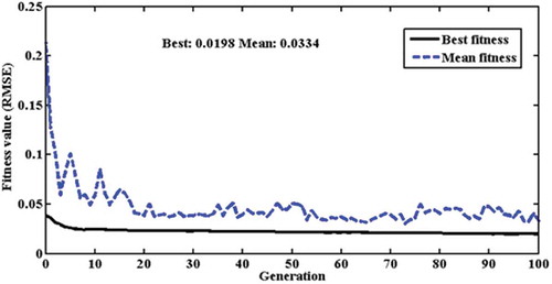
The GA-ANN model provided a set of final solutions at a pre-defined stopping criterion corresponding to maximum generations (100). The variation of the best fitness value (RMSE) and mean fitness in each generation in the training phase is shown in Figure 4. The best fitness amongst all generations was 0.0198 (mean: 0.0334). It was also observed that the best fitness function of each generation of genetic learning is unchanged after 10 generations (Fig. 4). The best chromosome corresponding to the best fitness function demonstrated that all the input parameters (water discharge, rainfall and temperature), need to be selected for developing the neural network model. The results also demonstrated that the optimum number of neurons in the hidden layer was 11. The tan-sigmoid activation function, which is an S-shaped curve, continuous and monotonically increasing, was optimally selected as an activation function for both the hidden and output layers. The optimized value of the combination coefficient (µ) in the LM algorithm model was selected as 10 by the GA-ANN model. The initial connection weights and bias terms were selected optimally, and in this case the number of terms was 56. The solution of the best-fit chromosomes after the evolution run was used as the optimal solution from the GA-ANN model.

Figure 4. Generation-wise fitness function profile during GA-based neural network learning.

To test the statistical similarities between actual data and the model-predicted sediment yields dataset, a paired sample t-test was conducted. If the significance level value of this test is lower than 0.05, then it could be concluded that the model-predicted sediment yield values are significantly different from the actual observation. It is observed from Table 5 that the GA-ANN model provided low t values (–0.4058 to 0.4837) with a high significance level (p = 0.6290–0.8968). The significance values of these datasets are greater than 0.05 for all paired sample tests. Hence, it confirms that the observed and estimated suspended sediment yield data are statistically similar for all training, validation and testing phases.

Table 5. Paired t-test between the observed and GA-ANN estimated values for training, validation and testing. Df: degree of freedom; SD: standard deviation.

	t-test statistic	p	Df	SD
Training	0.4837	0.6290	266	0.1535
Validation	–0.1303	0.8968	56	0.1285
Testing	–0.4058	0.6864	56	0.1274

The generalization capability and the performance of this developed GA-ANN model was evaluated with the test dataset. The statistical analysis of errors, which were calculated from the observed and model-predicted suspended sediment yields for the training, validation and testing datasets, is shown in Table 6. It may be seen in Table 6 that the RMSE is very low and R² is very high for all three datasets. The mean absolute error (MAE) is also very low and consistent amongst all three datasets. Based on the RMSE, MAE and R² values, it is concluded that this GA-ANN model has achieved good accuracy in the prediction of the suspended sediment yield. The consistency of all parameters amongst all three datasets demonstrated that the developed model has a generalization capability. From the low error parameter values and high R² values during the training, validation and testing, it was established that both overfitting and underfitting are prevented for this model.

Table 6. Error statistics of the GA-ANN model for Tikarapara station. RMSE: root mean square error; R²: coefficient of determination; MAE: mean absolute error; MSE: mean square error.

Statistics	Training	Validation	Testing
RMSE	0.0554	0.0198	0.02675
R^2	0.9267	0.9777	0.9923
MAE	0.0267	0.0129	0.0146
Mean error	–0.00907	0.00440	0.01357
Error variance	0.00301	0.00039	0.00056
MSE	0.00307	0.00039	0.00072

The optimum GA-ANN model was used to predict the sediment yield values at different time periods (monthly) from March 2001 to July 2003 using water discharge, rainfall and temperature as the input parameters for the model. The observed and model-predicted sediment yields are presented in Figure 5(a), which clearly shows the maximum number of times the sediment yield is overestimated. There are only two months (September and November 2001) when it was underestimated. The mean absolute relative error (MARE) was found to be 0.1495 at peak sediment yield, which is very low. Thus, it may be inferred that the GA-ANN model also provides a very accurate result at the peaks.

Figure 5. (a) Comparison and (b) scatter plot between observed and GA-ANN estimated sediment yield based on testing data.

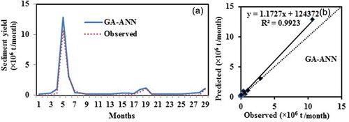
The GA-ANN model predicted the first maximum peak as 12 876 196 t/month (observed: 10 698 912 t/month) with a 20.35% overestimation. The GA-ANN prediction of the second maximum peak (1 177 535 compared to 1 074 786 t/month) was a 9.56% overestimation. This overestimation may be due to the presence of a large number of higher sediment yield values in training datasets (X_max/X_mean = 15.72, where X_max = 17 346 901 t/month and X_mean = 1 103 442 t/month. It is also observed that an estimated value of sediment yield is close to the observed values (Fig. 5(a)). The scatter plot between the observed and predicted suspended sediment yield using the GA-ANN model is shown in Figure 5(b). It is seen that most of the points lie along the bisector line, where both predicted and observed values are approximately the same. However, in one month, July 2001, an abnormally high estimated sediment yield of 12 876 196 t/month was obtained, which might be due to a higher water discharge (11 786 m³/s) and heavy rainfall (939 mm). This overestimation was confirmed by the positive mean error (0.0146) of the GA-ANN model in the testing phase. Zhu et al. (2007) also observed overestimated suspended sediment flux by the neural network model when using data from the Longchuanjiang River in the Upper Yangtze catchment, China. Adib and Jahanbakhshan (2013) and Adib and Mahmoodi (2017) also found overestimated suspended sediment concentration and suspended sediment load while using data from tidal rivers (Karun and Marun in Iran, respectively).

4.2 GA-SVM

The setting of the SVM parameters plays a very important role for the learning and generalization capability of the model. Water discharge, rainfall and temperature are selected as optimum input parameters in the GA-SVM model, as in the GA-ANN model. The optimum C and ɛ values in the GA-SVM model are 10 and 0.001, respectively. It is observed that the value of C is significantly high, which indicates that the trade-off term giving the regularized term is more important than the sum of the square error (SSE) term. The SSE term always tries to minimize the error between the training data and the fitted model. Thus, if SSE terms are given more importance, then they may lead to the model’s overfitting, which is less generalized. Giving more importance to the regularized term ensures the generalization of the model. The Gaussian kernel function was selected as the optimum kernel in the GA-SVM model.

The error statistics (RMSE, R², MAE, MSE, error variance and mean error) of the training, validation and testing datasets of the GA-SVM model were calculated using standard formulas (Legates and McCabe 1999, Sahoo and Jha 2013) and are presented in Table 7. It is observed from Table 7 that the RMSE, MSE, error variance, mean error and MAE for the GA-SVM model are very low, while R² is very high for all three datasets. These results confirm that the GA-SVM model can also predict the suspended sediment yield with high accuracy.

Table 7. Error statistics of the GA-SVM model for Tikarapara Station.

Statistics	Training	Validation	Testing
RMSE	0.043711	0.02612	0.02665
R^2	0.93607	0.970989	0.96295
MAE	0.015837	0.01223	0.012449
Mean error	–0.00281	0.010207	0.004113
Error variance	0.001917	0.000599	0.000718
MSE	0.001911	0.00068	0.000710

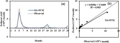
Figure 6 presents the actual and estimated values of the sediment yield using the GA-SVM model, indicating the maximum numbers of times the sediment yield is overestimated. It is clear from Figure 6(a) that very high underestimation and deviation are found at the first peak, i.e. the highest peak. It is also found that a high overestimation and deviation occurred at the second peak. It can be seen in Figure 6(b) that some points are below the 45 degree line and have negative values at the points where the sediment yield is low. The fitted line also shows significance bias in the model prediction. It is demonstrated that this model has reduced capability to predict at very high sediment values, as compared to the GA-ANN model. It is clear from Figure 6(a) that the GA-SVM model provided negative sediment at low sediment values at index 2, 3 and 27. Figure 6(b) also shows that the GA-SVM model generates a negative value at some points where the sediment is low.

Figure 6. (a) Comparison and (b) scatter plot between observed and GA-SVM estimated sediment yield based on testing data.

4.3 MLR

The MLR model was developed with the use of the training datasets. Since the linear model does not overfit, a validation dataset is not required. The same test data as were used for the GA-ANN, GA-SVM, SVM and ANN models were used for testing purposes. In total, seven MLR models were developed by selecting different combinations of input variables out of water discharge (Q), rainfall (R) and temperature (T). The RMSE values of all seven models for the training dataset are shown in Figure 7. It is observed from Figure 7 that the minimum RMSE was obtained when a combination of water discharge and rainfall (Q + R) was taken as input. Upon combining temperature with water discharge (Q + T), no significant improvement was observed in the models; however, for Q + R, a relatively small improvement was observed in the predicting power of the linear model. The estimated coefficients (a, b and c) of the best MLR model with the selected inputs (Q + R) are –0.0223, 0.8644 and 0.0349, respectively.

Figure 7. Variation of RMSE using MLR models.

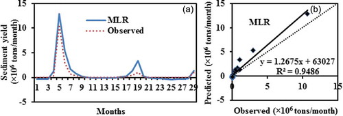
For comparison purposes, the best MLR model was used to predict sediment yield values for the testing dataset and the calculated error statistics are presented in Table 8; a comparison between observed and estimated SSY is presented in Figure 8. It may be seen that the MLR model provides a negative value at the points where the sediment yield is low (Fig. 8). Figure 8(b) shows that most of the data points lie along the bisector line, where both predicted and observed values are the same. However, there is an overestimation of the sediment yield beyond 1 016 919 t/month. This reveals that the data have a strong nonlinear behaviour in the area of small valued samples. The linear MLR model failed to capture the nonlinearity of the suspended sediment and estimated a negative value of the sediment yield.

Table 8. Error statistics of the MLR model for Tikarapara station.

Statistics	Training	Validation	Testing
RMSE	0.0575	0.0557	0.0476
R^2	0.8853	0.9301	0.9486
MAE	0.0288	0.0346	0.0286
Mean error	1.1651 × 10^−18	0.0223	0.0136
Error variance	0.00334	0.00270	0.00216
MSE	0.00331	0.00310	0.00227

Figure 8. (a) Comparison and (b) scatter plot between observed and MLR estimated sediment yield based on testing data.

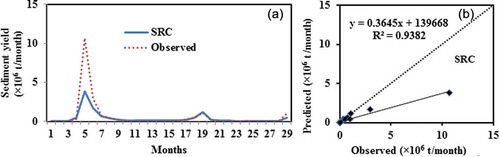
4.4 SRC

The coefficient of the SRC curve was estimated using the least square regression in the log scale then back-transfer was applied for the original scale. The estimated values of coefficients a and b are 0.2577 and 0.9576, respectively, for this model. Table 9 lists the error statistics of the proposed model, showing that the SRC model during the training phase has a lower value of R² and a higher RMSE, whereas in the testing phase RMSE was lower and R² higher. From the hydrograph and scatter plot between the observed and predicted SSY, it may be seen that the SRC model provides an underestimated value at a very high sediment yields (Fig. 9). This underestimation behaviour is also inferred by the negative mean error values. As seen in the scatter plot (Fig. 9(b)), the slope of the regression line is less than 1 (slope of bisector line) and the points mostly fall along the bisector line; however, at high sediment values they are highly underestimated, falling far below the line. A similar underestimation of the suspended sediment predicted value was also obtained in some river basins in the USA (Rajaee et al. 2009, Kisi and Guven 2010). This deviation is mainly caused by the consideration of only water discharge as an input variable over all other parameters that play a direct or indirect role in producing sediment to the river.

Table 9. Error statistics of the SRC model for Tikarapara station.

Statistics	Training	Testing
RMSE	0.1270	0.0752
R^2	0.8721	0.9382
MAE	0.0449	0.0193
Mean error	–0.0411	–0.0156
Error variance	0.01452	0.00561
MSE	0.01612	0.00566

Figure 9. (a) Comparison and (b) scatter plot between observed and SRC estimated sediment yield based on testing data.

4.5 ANN

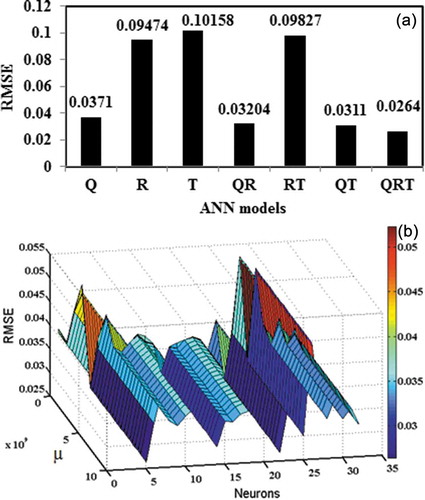
The LM-based MLP neural network models were developed through input and output neurons with a single hidden layer. The number of neurons in the hidden layer, and the combinational coefficient of the ANN model were selected by the grid search algorithm. Seven different models were attempted by combining the same three variables (Q, R and T). The results demonstrate that the water discharge is the most influential factor for sediment yield prediction; however, inclusion of rainfall and temperature in the ANN model improved the predictive capability of the model (Fig. 10(a)), which shows that the ANN model produced a minimum RMSE value (0.0264) in the validation data when water discharge, rainfall and temperature (Q + R + T) were considered as input parameters. Therefore, this was considered as the best ANN model amongst all seven models. During this ANN study, the value of the combination coefficient (µ) was variable, from 0.001 to a maximum of 9 × 10⁹, being increased and decreased by a factor of 10 and 0.1, respectively. The model started with an initialized µ value, which then changed in each epoch to improve the performance. The RMSE values of the grid search algorithm are presented in Figure 10(b), which constitutes a trade-off between the hidden node number and combination coefficient value. It was observed that the optimum value of hidden neurons is 5 and the value of µ is 0.01.

Figure 10. (a) Variation of RMSE using ANN models. (b) Effect of µ and number of neurons on RMSE for the ANN model.

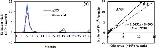
The error statistics (RMSE, R², MAE, MSE and error variance) of the training, validation and testing datasets of the ANN model are presented in Table 10. It may be seen from Table 10 that the RMSE and MAE for the ANN model are very low, while R² is very high for all three datasets. These results confirm that the ANN model can also predict the SSY with high accuracy. The low RMSE and MAE values and high R² values of the training, validation and testing datasets are approximately close to each other, confirming that the developed model is not underfitted or overfitted. According to the paired sample t-test result, the observed and ANN estimated SSY for training, validation and testing datasets are also statistically similar, with low t values in the range –0.2187 to 0.4450 and high significance (p = 0.6567–0.8980) based on the 0.05 level of significance.

Table 10. Error statistics of the ANN model for Tikarapara station.

Statistics	Training	Validation	Testing
RMSE	0.0425	0.0264	0.0419
R^2	0.9410	0.9717	0.9948
MAE	0.0201	0.0164	0.0157
Mean error	−0.0090	0.0046	0.0080
Error variance	0.00174	0.00070	0.00175
MSE	0.00181	0.00070	0.00176

It may be seen that overestimations occur only at the peaks (Fig. 11(a)); however, the over- or underestimations are not very significant. It is also clear from Figure 11(a) that the predicted and observed SSY values are similar. The scatter plot between the actual and model estimated values (Fig. 11(b)) shows most of the points are close to the bisector line. The slope of the regression line is greater than 1, which indicates that overestimation occurs. It is also noted that the ANN model predicted a negative sediment yield at low value.

Figure 11. (a) Comparison and (b) scatter plot between observed and ANN estimated sediment yield based on testing data.

4.6 SVM

In total seven SVM models were developed by changing the input variables and selecting other SVM hyper-parameters using the grid search algorithm. Figure 12 shows the RMSE values for all seven models; the minimum RMSE (0.04368) was obtained when water discharge, rainfall and temperature were taken as input variables (Q + R + T). The same sets of variables were also selected in the ANN, GA-ANN and GA-SVM models. The values of C and ɛ were selected as 1 and 0.0027, respectively, and the linear kernel function was selected by the grid search method.

Figure 12. Variation of RMSE for SVM models.

The error statistics of training, validation and test datasets are presented in Table 11. It is clear from Table 11 that the traditional SVM model provided satisfactory performance with low RMSE, MSE, MAE, error variance and mean error and high R² values. However, it should be noted that the process takes a large amount of computational time to select inputs, the kernel function, and hyper-parameters for the SVM model.

Table 11. Error statistics of the SVM model for Tikarapara station.

Statistics	Training	Validation	Testing
RMSE	0.06118	0.04368	0.03442
R^2	0.88456	0.92729	0.94755
MAE	0.02432	0.02604	0.01896
Mean error	0.00061	0.01983	0.01579
MSE	0.00374	0.00191	0.00119
Error variance	0.00377	0.00157	0.00096

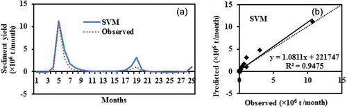
Figure 13 presents the observed and estimated values of the sediment yield using the traditional SVM model; the maximum number of times the predicted sediment yield values were overestimated is also shown (Fig. 13(a)). It may also be seen that the estimated SSY is not as close to the observed SSY as in the GA-ANN and GA-SVM models. There is greater overestimation at the second peak with the SVM model compared to the GA-based models. The slope of the regression line is greater than 1, which indicates that overestimation occurs (Fig. 13(b)). This result is also supported by the positive mean error value (Table 11). It is also seen from Figure 13(b) that some points are below the 45 degree line and have negative values at the points where the sediment yield is low. This demonstrates that the data have a strong nonlinear behaviour in the small-valued sample area. The SVM model failed to capture that complex nonlinearity, which resulted in some negative estimated values, as for the ANN and MLR models. This is due to the selection of a linear kernel function by means of the grid search method. It is observed that the SVM model generated a negative value of SSY at the low valued sample area; however, the sediment yield can never be negative in reality. In contrast, the GA-ANN model generated a positive sediment value even when the suspended sediment yield is low.

Figure 13. (a) Comparison and (b) scatter plot between observed and SVM estimated sediment yield based on testing data.

4.7 Comparative evaluation of the different models on testing data

After the reliable GA-ANN model development, the performance of the models was examined using the test dataset, which is excluded from the training stage. To evaluate the performance of this proposed simultaneous optimization of all related parameters in the sediment yield prediction using the GA-ANN and GA-SVM models, they were compared with those of MLR, SRC and the traditional ANN and SVM models. The same test dataset was used in all the models for comparison, which was based on the estimated values of the test data. The error statistics obtained during testing using the above models are presented in Table 12. It may be seen that the GA-ANN performed better in terms of minimizing the RMSE and MAE than the traditional neural network and regression models (Table 12). It is also shown in Table 12 that the prediction model error performance (RMSE) of the ANN model is decreased when it is used in conjunction with the GA in the testing phase. Similarly, the RMSE of the SVM model is reduced when the GA is used in the SVM model for selecting all parameters simultaneously. The GA-ANN and GA-SVM models reduced the error by 36.28 and 22.38% compared to the traditional ANN and SVM models, respectively. Thus, both the GA-ANN and GA-SVM models provided better results than the ANN and SVM models, respectively, by considering the optimum input variables and associated parameters. This superiority is due to the optimization of all ANN and SVM parameters simultaneously using the GA. However, although R² is very high (0.9923), the GA-ANN is still next to the ANN, which has a maximum R² value (0.9948). Based on only R², it is not always possible to evaluate the capability of a model (Legates and McCabe 1999, Zhu et al. 2007, Sahoo and Jha 2013). The GA-ANN and the GA-SVM based linear regression lines are very close to the 1:1 lines of the ANN and SVM based models, respectively, as observed in the scatter plots (Figs. 5(b), 6(b), 11(b) and 13(b)).

Table 12. Comparison of the performance of the six models for the testing period. Bold values indicate the best performance.

Model	Input	RMSE	R^2	MAE	Optimum model parameters*
GA-ANN	Q, R, T	0.0267	0.9923	0.0146	NN: 11; CC: 10; TF: tan-sigmoid and tan-sigmoid, HL: 1; CP: 0.6; MP: 0.05; G: 100; PS: 50
ANN	Q, R, T	0.0419	0.9948	0.0157	NN: 5; CC: 0.01; TF: tan-sigmoid and pure linear; HL: 1
GA-SVM	Q, R, T	0.0267	0.9630	0.0125	C: 0.001; ε: 10; KF: Gaussian
SVM	Q, R, T	0.0344	0.9475	0.0190	C: 0.0027; ε: 1; KF: linear
MLR	Q, R	0.0476	0.9577	0.0286	a: – 0.0223; b: 0.8644; c: 0.0349
SRC	Q	0.0752	0.9382	0.0193	a: 0.2577; b: 0.95769

* NN: number of nodes in hidden layer; CC: combination coefficient; TF: transfer function; HL: hidden layers; CP: cross-over probability; MP: mutation probability; G: maximum number of generations; PS: population size; C: regularization parameter; KF: kernel function; ε: parameter ε in SVM.

In the hydrographs, it is also shown that the estimated sediment yield by the GA-ANN, GA-SVM, SVM and ANN models is closer to the observed data than the MLR and SRC, especially at high sediment values (Figs. 5(a), 6(a), 8(a), 9(a), 11(a) and 13(a)). The SRC model gave poor results and significantly underestimated the peaks; it was unable to capture the unusually high suspended sediment. In the scatter plot, it is seen that the ANN, SVM, GA-SVM and MLR models estimated negative suspended sediment at low values, similar to the results of past research (Cigizoglu 2004, Cigizoglu and Kisi 2006, Sharma et al. 2015). This is completely unrealistic as the suspended sediment yield cannot be negative in nature. However, the GA-ANN model provided a positive sediment value even when the SSY was low. The negative sediment estimates that were encountered in the soft computing calculations were not produced by this method. These results indicate that the GA-based neural network approach may give better performance and generalization capability than the other methods applied in this research. Thus, the GA-ANN appears to be the most capable model compared to other studied models.

The MARE values of the GA-ANN, ANN, GA-SVM, SVM, MLR and SRC models are 0.1495, 0.460314, 0.3326, 0.9670, 1.1601 and 0.3567, respectively, at peak sediment yield values. Thus the GA-ANN model has the lowest MARE, while the MLR model has a maximum MARE at peak SSY values. These results also show that both the GA-ANN and GA-SVM models have a smaller MARE value than the ANN and SVM model, respectively. This indicates that both GA-ANN and GA-SVM perform better than the latter models.

The error in the total SSY estimated using the six models (GA-ANN, ANN, GA-SVM, SVM, MLR and SRC) is higher than the observed value (18 654 005 t) in the testing phase (by 36.6, 29.6, 11.1, 42.6 and 34%, respectively) for the first five models and lower (by 41.8%) for the SRC model. Here, both positive and negative estimated SSY by each model are considered corresponding to observing the SSY using the test dataset. According to these results, the GA-SVM has the lowest error and seems to be the best model. However, the SSY can never be negative in reality and the negative estimated value compensates the over- and underestimation of the models. Thus, by considering only the positive estimated SSY values for calculating the error in the total sediment load estimation, the results for the GA-ANN, ANN, GA-SVM, SVM, MLR and SRC models are 19.8, 31, 9.56, 44.91 and 58.3% higher and 45.8% lower (compared to the observed values in the test dataset). This indicates that the GA-SVM model has the lowest error in the estimation of the suspended sediment yield.

To test statistical similarities between the estimated and observed values for the test dataset, the t-test and ANOVA test were performed. Researchers have argued that if the ANOVA test and t-test results between the observed and estimated sediment yield are both significant then the model is robust (Kisi 2005, Cobaner et al. 2009). The results of the t-test for the studied models (GA-ANN, ANN, GA-SVM, SVM, MLR and SRC) are 0.2356, 0.3468, 0.1237, 0.4921, 0.6018 and –0.7601, respectively, and those of the ANOVA are 0.0555, 0.1203, 0.0153, 0.2456, 0.3621 and 0.5778, respectively (p = 0.8157, 0.7317, 0.9026, 0.6272, 0.553 and 0.4546, respectively for both tests).

The results of both tests reveal that the GA-ANN model gave smaller values, with a high significance level (0.8157), while the GA-SVM model gave the smallest values, with the highest significance level (0.9026); however, these results do not differ greatly. The t-test and ANOVA results for both the GA-ANN and GA-SVM models are smaller, with a higher significance value, than the ANN and SVM models, respectively. Both tests are set at a 95% significance level, namely the differences between the observed and estimated values were considered significant when the resultant significance level (p) was lower than 0.05 by use of paired significance levels. Thus the GA-ANN and GA-SVM models are the most robust (the similarity between the observed and estimated SSY is significantly high) in comparison to the other models in estimating the suspended sediment yield. Thus, both observed and estimated suspended sediment yields are statistically similar in nature. The observed and estimated suspended sediment yields have the same distributions.

5 Conclusion

This study has demonstrated the estimation of suspended sediment yields by GA-ANN, GA-SVM, ANN, SVM, MLR and SRC models using different inputs of hydroclimatic variables (water discharge, rainfall and temperature) at the Tikarapara gauge station in the Mahanadi River basin, India. It was found that water discharge, rainfall and temperature are the most dominant controlling parameters of the suspended sediment in the Mahanadi River. Climate change could affect the sedimentation process in a river.

A different ANN structure was considered for the determination of the suspended sediment yield and the utilization of the GA efficiently optimized this structure. Traditional MLR and SRC models did not provide a satisfactory prediction of the suspended sediment yield.

The GA-ANN model can provide a more reasonable prediction for extremely high or low values of suspended sediment as compared to the ANN, GA-SVM, SVM, MLR and SRC models. This research also suggests that a network with one hidden layer (11 nodes) is the optimum network for the GA-ANN model, which provided the best results.

It is proposed that the GA-ANN (RMSE-0.0267 and MAE-0.0146) and GA-SVM (RMSE-0.0267 and MAE-0.0125) models can be potential substitutes for conventional models such as the ANN (RMSE-0.0419 and MAE-0.0157), SVM (RMSE-0.03442 and MAE-0.0190), MLR (RMSE-0.0476 and MAE-0.0286) and SRC (RMSE-0.0752 and MAE-0.0193) models. The implementation of the artificial neural network and support vector machine methods in the present study has demonstrated their flexibility and ability to model the nonlinear relationship between the input and output variables for sediment yield prediction. The proposed GA-ANN and GA-SVM models predict the sediment yield reasonably well using water discharge, rainfall and temperature simultaneously as inputs.

Overall, the magnitude of low, medium and high SSY prediction by the GA-ANN and GA-SVM models was closer to the observed values (Fig. 5(a) and 6(a)). The GA-ANN and GA-SVM estimated sediment yield values are closer to the observed SSY than those estimated by the other models. The GA-ANN and GA-SVM models provided satisfactory performance and had higher generalization capability. This superiority was due to the optimization of all ANN and SVM parameters simultaneously using the GA.

Also, the GA-ANN, GA-SVM, SVM and ANN models provided better results than the MLR and SRC models for estimating the sediment yield. Therefore, optimizing both the SVM and ANN parameters and input subsets simultaneously with the genetic algorithm is a better approach than the traditional method of trial-and-error and grid search method for selecting input variables and other parameters associated with the models. This study shows that parameter selection not only improves the performance of the model but also significantly reduces the computational time by eliminating the grid search and trial-and-error exercise.

The major contribution of this research is the simultaneous optimization of parameters and input variables for sediment yield prediction modelling. The approach used herein has been tested in other application domains; however, this study focused on sediment yield prediction, which is the unique contribution of this research. Moreover, this research is original in terms of study area, data used and results obtained. Our results have practical importance in the sense that the trained ANN and SVM models using the GA based on simple inputs (water discharge, rainfall and temperature data) can be used for the estimation of monthly sediment yield in the Mahanadi basin. Estimation on a watershed level will help in facilitating effective watershed management. This approach will be useful for better management of water resources for the downstream area as well as for the design of dams, pipes, canals, bridges, water treatment processes, stream geomorphology, and evaluation of water quality problems in the Mahanadi River, India.

The study only used data from one gauge station and further work using more data from various gauge stations may be required in order to strengthen these conclusions. In future research, other kinds of ANN will be tested and new datasets will be introduced to the models.

Acknowledgements

The authors would like to express their thanks to the Central Water Commission (CWC), Bhubaneswar, which provided the data for this study. In addition, the authors wish to acknowledge the National Institute of Technology, Rourkela, for providing financial support in the form of a fellowship and facility needed during this study.

Disclosure statement

No potential conflict of interest was reported by the authors.

References

- Adeloye, A. and Munari, A.D., 2006. Artificial neural network based generalized storage yield- reliability models using the Levenberg-Marquardt algorithm. Journal of Hydrology, 362, 215–230.
- Adib, A. and Jahanbakhshan, H., 2013. Stochastic approach to determination of suspended sediment concentration in tidal rivers by artificial neural network and genetic algorithm. Canadian Journal of Civil Engineering, 40, 299–312.
- Adib, A. and Mahmoodi, A., 2017. Prediction of suspended sediment load using ANN GA conjunction model with markov chain approach at flood conditions. KSCE Journal of Civil Engineering, 21 (1), 447–457.
- Admuthe, L., Apte, S., and Admuthe, S., 2009. Topology and parameter optimization of ANN using genetic algorithm for application of textiles. In: IEEE international workshop on intelligent data acquisition and advanced computing systems: technology and applications, 2009. IDAACS 2009. Piscataway, NJ: IEEE Operations Center, 278–282. doi:10.1109/IDAACS.2009.5342981
- Ahmadi, H. and Rodehutscord, M., 2017. Application of artificial neural network and support vector machines in predicting metabolizable energy in compound feeds for pigs. Frontiers in Nutrition, 4, 27. doi:10.3389/fnut.2017.00027
- Altun, H., Bilgil, A., and Fidan, B.C., 2007. Treatment of multidimensional data to enhance neural network estimators in regression problems. Expert Systems with Applications, 32 (2), 599–605.
- Altunkaynak, A., 2008. Adaptive estimation of wave parameters by Geno-Kalman filtering. Ocean Engineering, 35, 1245–1251.
- Altunkaynak, A., 2009. Sediment load prediction by genetic algorithms. Advances in Engineering Software, 40 (9), 928–934.
- Asadi, S., et al. 2013. A new hybrid artificial neural networks for Rainfall-Runoff process modeling. Neurocomputing, 121, 470–480.
- Bastia, F. and Equeenuddin, S.M., 2016. Spatio-temporal variation of water flow and sediment discharge in the Mahanadi River, India. Global and Planetary Change, 144, 51–66.
- Beyer, H.G., 2000. Evolutionary algorithms in noisy environments: theoretical issues and guidelines for practice. Computer Methods in Applied Mechanics and Engineering, 186 (2), 239–267.
- Bishop, M., 1998. Neural networks for pattern recognition. Oxford: Clarendon Press.
- Boukhrissa, Z.A., et al., 2013. Compare the Ann and Sediment rating curve model for prediction of suspended sediment load in EI Kebir catchment, Algeria. Journal of Earth Systems Science, 122 (5), 1303–1312.
- Buendia, C., et al. 2016. Effects of afforestation on runoff and sediment load in an upland Mediterranean catchment. Science of the Total Environment, 540, 144–157.
- Castillo, P.A., et al., 2000. G-prop: global optimization of multilayer perceptrons using GAs. Neurocomputing, 35 (1–4), 149–163.
- Chatterjee, S. and Bandopadhyay, S., 2007. Global neural network learning using genetic algorithm for ore grade prediction of iron ore deposit. Mining and Resource Engineering, 12 (4), 258–269.
- Chatterjee, S. and Bandopadhyay, S., 2011. Goodnews bay platinum resource estimation using least square support vector regression with selection of input space dimension and hyper-parameters. Natural Resources Research, 20, 117–129.
- Chatterjee, S. and Bandopadhyay, S., 2012. Reliability estimation using a genetic algorithm-based artificial neural network: an application to a laud-haul-dump machine. Expert Systems and Appllications, 39, 10943–10951.
- Chau, K.W., Wu, C., and Li, Y.S., 2005. Comparison of several flood forecasting models in Yangtze River. Journal of Hydrologic Engineering, 10 (6), 485–491.
- Chiu, D.Y. and Chen, P.J., 2009. Dynamically exploring internal mechanism of stock market by fuzzy-based support vector machines with high dimension input space and genetic algorithm. Expert Systems Applications, 36 (2), 1240–1248.
- Cigizoglu, H.K., 2004. Estimation and forecasting of daily suspended sediment data by multi-layer perceptrons. Advances in Water Resources, 27 (2), 185–195.
- Cigizoglu, H.K. and Kisi, Ö., 2006. Methods to improve the neural network performance in suspended sediment estimation. Journal of Hydrology, 317 (3), 221–238.
- Cobaner, M., Unal, B., and Kisi, O., 2009. Suspended sediment concentration estimation by an adaptive neuro-fuzzy and neural network approaches using hydro-metrological data. Journal of Hydrology, 367, 52–61.
- Correa, A., Gonzalez, A., and Ladino, C., 2011. Genetic algorithm optimization for selecting the best architecture of a multi-layer perceptron neural network: a credit scoring case. In: SAS global forum 2011 data mining and text analytics. Cary, NC: SAS Institute.
- Coulthard, T.J., Kirkby, M.J., and Macklin, M.G., 2000. Modelling geomorphic response to environmental change in an upland catchment. Hydrological Processes, 14 (11–12), 2031–2045.
- CWC (Central Water Commission), 2012. Integrated hydrological data book. Hydrological data directorate, information systems organization, Water planning and projects wing. In: Central water commission. New Delhi: Hydrological Data Directorate, Information System Organization, Water Planning and Projects Wing, Central Water Commission (CWC).
- Davis, L., 1991. Handbook of genetic algorithms. Graham: Van Nostrand Reinhold.
- Dejong, K., 1975. An analysis of the behavior of a class of genetic adaptive systems. Ph.D. dissertation. Department of Computer and Communication Sciences, University of Michigan.
- Demuth, H.B. and Beale, M., 1998. Neural network Toolbox for use with MATLAB, Users Guide. Massachusetts, USA: The Mathworks, Inc.
- Dibike, Y.B., et al., 2001. Model induction with sup-port vector machines: introduction and application. Journal of Computing in Civil Engineering, 15 (3), 208–216.
- Fatemi, M.H., Jalali-Heravi, M., and Konuze, E., 2003. Prediction of bioconcentration factor using genetic algorithm and artificial neural network. Analytica Chimica Acta, 486, 101–108.
- Ghose, D.K., Swain, D.P.C., and Panda, D.S.S., 2012. Sediment load analysis using ANN and GA. Applied Mechanics and Materials, 110-116, 2693–2698.
- Goldberg, D.E., 1989. Genetic algorithms in search, optimization, and machine learning. Boston, MA: Addison-Wesley Publishing Company Inc.
- Gupta, H., Kao, S.J., and Dai, M., 2012. The role of mega dams in reducing sediment fluxes: a case study of large Asian rivers. Journal of Hydrology, 464-465, 447–458. doi:10.1016/j.jhydrol.2012.07.038
- Gupta, J.N.D. and Sexton, R.S., 1999. Comparing backpropagation with a genetic algorithm for neural network training. Omega, 27, 679–684.
- Gupta, S.C. and Kapoor, V.K., 2013. Fundamental of mathematical statistics. New Delhi: Sultan Chand and Sons.
- Hagan, M.T. and Menhaj, M.B., 1994. Training feedforward networks with the Marquardt algorithm. IEEE Transactions on Neural Networks, 5 (6), 989–993.
- Haghizade, A., Shui, L.T., and Goudarzi, E., 2010. Estimation of yield sediment using artificial neural network at basin scale. Australian Journal of Basic and Applied Sciences, 4 (7), 1668–1675.
- Haji, M.S., et al., 2014. Suspended sediment modelling by SVM and wavelet. Građevinar, 66 (3), 211–223.
- Harrison, C.G.A., 2000. What factors control mechanical erosion rates? International Journal of Earth Sciences, 88 (4), 752–763.
- Heikamp, K. and Bajorath, J., 2014. Support vector machines for drug discovery. Expert Opinion on Drug Discovery, 9 (1), 93–104.
- Holland, J., 1975. Adaptation in natural and artificial systems. Ann Arbor, MI: The University of Michigan Press.
- Hornik, K., Stinchcombe, M., and White, H., 1989. Multilayer feed forward networks are universal approximators. Neural Networks, 2, 359–366.
- India-WRIS, 2015 Water resources information system of india[onlne]. Available from: http://india-wris.nrsc.gov.in/wrpinfo/index.php?title=Mahanadi [Accessed 2 April 2016].
- Jain, A. and Srinivasulu, S., 2004. Development of effective and efficient rainfall-runoff models using integration of deterministic, real-coded genetic algorithms and artificial neural network techniques. Water Resources Research, 40 (4), 1–12.
- Jain, S.K., 2001. Development of integrated sediment rating curves using ANNs. Journal of Hydraulic Engineering, 127 (1), 30–37.
- Jansson, M.B., 1997. Comparison of sediment rating curves developed load and on concentration. Nordic Hydrology, 28 (3), 189–200.
- Jin, Y., Sendhoff, B., and Körner, E., 2005. Evolutionary multi-objective optimization for simultaneous generation of signal-type and symbol-type representations. In: Coello C.A.C., Aguirre, A.H., and Zitzler, E., eds. Proceedings of the 3rd international conference on evolutionary multi-criterion optimization. New York: Springer- Verlag, 752–766, Lecture Notes in Computer Science, 3410.
- Kafle, K.R., Khanal, S.N., and Dahal, R.K., 2015. Dynamics of the Koshi river on the perspective of morphology and sedimentation with emphasis on post disaster impact of the 2008 Koshi flood. Journal of Science, Engineering and Technology, 11 (1), 71–92.
- Kar, A.K., et al. 2010. Development of flood forecasting system using statistical and ANN techniques in the downstream catchment of Mahanadi Basin, India. Journal of Water Resource and Protection, 2, 880–887.
- Kashid, S.S., Ghosh, S., and Maity, R., 2010. Streamflow prediction using multisite rainfall obtained from hydroclimatic teleconnection. Journal of Hydrology, 395, 23–38.
- Khan, M.Y.A., et al., 2016. Neural network model for discharge and water-level prediction for Ramganga River catchment of Ganga Basin, India. Hydrological Science Journal, 61 (11), 2084–2095.
- Khoi, D.N. and Suetsugi, T., 2014. The responses of hydrological processes and sediment yield to land-use and climate change in the Be River Catchment, Vietnam. Hydrological Processes, 28, 640–652.
- Kim, K.J. and Ahn, H., 2012. Simultaneous optimization of artificial neural networks for financial forecasting. Applied Intelligence, 36 (4), 887–898.
- Kisi, O., 2005. Suspended sediment estimation using neuro-fuzzy and neural network approaches. Hydrological Science Journal, 50 (4), 683–696.
- Kisi, O. and Guven, A., 2010. A machine code based genetic programming for suspended sediment concentration estimation. Advances in Engineering Software, 41, 939–945.
- Kisi, O. and Shiri, J., 2012. River suspended sediment estimation by climatic variables implication: comparative study among soft computing techniques. Computers and Geoscience, 43, 73–82.
- Legates, D.R. and McCabe, G.J., 1999. Evaluating the use of goodness-of-fit measures in hydrology and hydroclimatic model validation. Water Resource Research, 35 (1), 233–241.
- Lenzi, M.A. and Marchi, L., 2000. Suspended sediment load during floods in a small stream of the Dolomites (northeastern Italy). CATENA, 39 (4), 267–282.
- Li, X.Z. and Kong, J.M., 2014. Application of GA-SVM method with parameter optimization for landslide development prediction. Natural Hazards and Earth System Sciences, 14 (3), 525–533.
- Maniezzo, V., 1994. Genetic evolution of the topology and weight distribution of neural networks. IEEE Transactions on Neural Network, 5 (1), 39–53.
- Mathwork., 2012. MathWorks announces release 2012a of the MATLAB and simulink product families[online]. Available from: https://in.mathworks.com/company/newsroom/mathworks-announces-release-2012a-of-the-matlab-and-simulink-product-families.html [Accessed 7 July 2016].
- Meher, J., 2014. Rainfall and runoff estimation using hydrological models and ANN techniques. Ph.D. thesis. National institute of technology, Rourkela, 1–218.
- Meher, J. and Jha, R., 2013. Time series analysis of monthly rainfall data for the Mahanadi river basin, India. Sciences in Cold and Arid Regions, 5 (1), 73–84.
- Milliman, J.D. and Syvitski, J.P.M., 1992. Geomorphic/tectonic control of sediment discharge to the ocean: the importance of small mountainous rivers. The Journal of Geology, 100, 525–544. doi:10.1086/629606
- Parasuraman, K. and Elshorbagy, A., 2007. Cluster-based hydrologic prediction using genetic algorithm-trained neural networks. Journal Hydrologic Engineering, 52–62. doi:10.1061/(ASCE)1084-0699(2007)12:1(52)
- Patel, A.K., Chatterjee, S., and Gorai, A.K., 2017. Development of machine vision-based ore classification model using support vector machine (SVM) algorithm. Arabian Journal of Geosciences, 10 (5), 107.
- Pramanik, N. and Panda, R.K., 2009. Application of neural network and adaptive neuro-fuzzy inference systems for river flow prediction. Hydrological Science Journal, 54 (2), 247–260.
- Rajaee, T., et al. 2009. Daily suspended sediment concentration simulation using ANN and neuro-fuzzy models. Science of Total Environment, 407, 4916–4927.
- Rojas, R., 1996. Neural network: a systematic introduction. Berlin: Springer Verlag, 151–184.
- Sahoo, S. and Jha, M.K., 2013. Groundwater-level prediction using multiple linear regression and artificial neural network techniques: a comparative assessment. Hydrogeology Journal, 21 (1865), 1887.
- Sandy, R., 1990. Statistics for business and economics. New York: McGraw-Hill publishing, 1117.
- Saunders, C., et al., 1998. Support vector machine – reference manual royal holloway technical report CSD-TR-98-03. London: Royal Holloway.
- Sedki, A.D., Ouazar, D., and Mazoudi, E., 2009. Evolving neural network using real coded genetic algorithm for daily rainfall-runoff forecasting. Expert Systems and Applications, 36, 4523–4527.
- Sharma, N., et al., 2015. Runoff and sediment yield modeling using ANN and support vector machines: a case study from Nepal watershed. Modeling Earth Systems and Environment, 1 (3), 23.
- Singh, G. and Panda, R., 2011. Daily sediment yield modeling with artificial neural network using 10-fold cross validation method: a small agricultural watershed, Kapgari, India. International Journal of Earth Sciences and Engineering, 6 (4), 443–450.
- Sirdari, Z.Z., Ghani, A.A., and Sirdari, N.Z., 2015. Bedload transport predictions based on field measurement data by combination of artificial neural network and genetic programming. Pollution, 1 (1), 85–94.
- Smola, A.J., 1996. Regression estimation with support vector learning machines,Master’s thesis. Technische Universität München.
- Su, J., et al., 2013. GA-based support vector machine model for the prediction of monthly reservoir storage. Journal of Hydrologic Engineering, 19 (7), 1430–1437.
- Syvitski, J.P.M., et al., 2003. Predicting the terrestrial flux of sediment to the global ocean: a planetary perspective. Sedimentary Geology, 162 (1–2), 5–24.
- Tahmasebi, P. and Hezarkhani, A., 2009. Application of optimized neural network by genetic algorithm, IAMG09. California: Stanford University.
- Tang, Z., Almeida, D.C., and Fishwick, P.A., 1991. Time series forecasting using neural networks vs. Box- Jenkins methodology. Journal of Simulation, 57, 303–310.
- Vapnik, V.N., 1995. TheNature of Statistical LearningTheory. New York: Springer.
- Walling, D.E., 1978. Suspended sediment and solute response characterstics of the river Exe, Devon, England. In: R. Davidson-Arnott and W. Nickling, eds. Research in fluvial geomorphology (Proceeding of the 5th Guelph symposium. on geomorphology). Norwich, UK: Geo Abstracts, 169–197.
- Walling, D.E., 2009. The impact of global change on erosion and sediment transport by rivers: current progress and future challenges. Paris: United Nations Educational, Scientific and Cultural Organization.
- Wang, J., Liu, L., and Chen, J., 2008. Combination of genetic algorithm and support vector machine for daily flow forecasting. In: Fourth international conference on natural computation, 2008. ICNC’08. Jinan, China: IEEE, Vol. 2, 31–35. doi:10.1109/ICNC.2008.171.
- Yadav, A., Chatterjee, S., and Equeenuddin, S.M., 2017. Prediction of suspended sediment yield by artificial neural network and traditional mathematical model in Mahanadi river basin, India. Sustainable Water Resources Management, 1–15. doi:10.1007/s40899-017-0160-1
- Zanaganeh, M., Mousavi, S.J., and Sahidi, A.F.E., 2009. A hybrid genetic algorithm-adaptive neural network based fuzzy inference system in prediction of wave parameter. Engineering Applications of Artificial Intelligence, 22, 1194–1202.
- Zhang, D., et al. 2015. A genetic algorithm based support vector machine model for blood-brain barrier penetration prediction. BioMed Research International, 2015, 1–13.
- Zhao, M., et al., 2011. Feature selection and parameter optimization for support vector machines: a new approach based on genetic algorithm with feature chromosomes. Expert Systems with Applications, 38 (5), 5197–5204.
- Zhu, Y.M., Lu, X.X., and Zhou, Y., 2007. Suspended sediment flux modeling with artificial neural network: an example of the longchuanjiang river in the Upper Yangtze Catchment, China. Geomorphology, 84 (1–2), 111–125.
- Zhu, Y.M., Lu, X.X., and Zhou, Y., 2008. Sediment flux sensitivity to climate change: a case study in the Longchuanjiang catchment of the upper Yangtze River, China. Global and Planetary Change, 60 (3), 429–442.
- ZICL, 2014. Risk Nexus, Urgent case for recovery: what we can learn from the August 2014 Karnali River foods in Nepal. Zurich, Switzerland: Zurich Insurance Group Ltd.