Performance evaluation of satellite-based approaches for the estimation of daily air temperature and reference evapotranspiration

ABSTRACT

Different satellite-based radiation (Makkink) and temperature (Hargreaves-Samani, Penman-Monteith temperature, PMT) reference evapotranspiration (ET_o) models were compared with the FAO56-PM method over the Cauvery basin, India. Maximum air temperature (T_max) required in the ET_o models was estimated using the temperature–vegetation index (TVX) and an advanced statistical approach (ASA), and evaluated with observed T_max obtained from automatic weather stations. Minimum air temperature (T_min) was estimated using ASA. Land surface temperature was employed in the ET_o models in place of air temperature (T_a) to check the potency of its applicability. The results suggest that the PMT model with T_a as input performed better than the other ET_o models, with correlation coefficient (r), averaged root mean square error (RMSE) and mean bias error (MBE) of 0.77, 0.80 mm d⁻¹ and −0.69 for all land cover classes. The ASA yielded better T_max and T_min values (r and RMSE of 0.87 and 2.17°C, and 0.87 and 2.27°C, respectively).

KEYWORDS:

• reference evapotranspiration
• air temperature
• Penman-Monteith temperature
• Cauvery basin
• India

Editor R. Woods Associate editor P. Srivastava

1 Introduction

It is essential to assess the key components of the hydrological cycle and also to manage water resources efficiently at the basin scale. Thus, it is crucial to have an accurate estimation of reference evapotranspiration (ET_o) over the Cauvery basin, which is one of the important river basins of peninsular India. ET_o is a climatic factor, estimated from climatic variables such as air temperature (T_a), solar radiation (R_s), relative humidity and wind speed. Owing to the difficulty in direct measurement of ET_o, indirect methods have been proposed, classified on the basis of their requirements of climatic variables, such as combination-type, radiation-type, temperature-type and mass-transfer-type methods. The Penman-Monteith (PM) method of the Food and Agriculture Organization (FAO) (FAO56-PM) is a combination method, and has a record of deriving accurate ET_o in most climatic regions, since it considers all the above-mentioned climatic variables. It is also recommended as a standardized method by the FAO. Most of the climatic variables required for the FAO56-PM method are hard to obtain because of the difficulty in maintaining the prescribed hypothetical conditions required for the estimation of ET_o at weather stations. Hence, alternative methods have been proposed by various researchers (Blaney and Criddle 1962, Hargreaves and Samani 1985, De Bruin 1987), as these require fewer climatic variables and are readily available for most of the climatic conditions and regions. But many of these alternative methods are site-specific and require calibration before application to another region. Consequently, many researchers have compared various methods and validated them with the FAO56-PM method at point scale for their particular study region (Gavilan et al. 2006, Douglas et al. 2009, Aguilar and Polo 2011, Fotios and Andreas 2011, Valipour 2012, 2014, 2015a, 2015b, 2017, Todorovic and Pereira 2013, Raziei and Pereira 2013a, Kisi 2014, Senatore et al. 2015, Almorox et al. 2015, Valipour et al. 2017). In India, Nandagiri and Kovoor (2006) evaluated seven models for different ranges of Indian climate at the point scale.

Climatic variables obtained from meteorological stations are at the point scale. Using these, it is difficult to obtain spatial variations of ET_o. Even though spatial interpolation techniques have been developed to obtain spatial variations of climatic variables, these require a dense network of high-quality meteorological stations (Raziei and Pereira 2013b). Such networks are costly to install and maintain in developing countries. In contrast, remote sensing techniques can provide the required data for estimation of ET_o at high spatial and temporal resolution in a feasible way. Hence, some authors have proposed a simplified methodology for the estimation of ET_o using remotely sensed data, employing available ET_o models. Rivas and Caselles (2004) examined the utility of land surface temperature (LST) over Argentina to estimate spatial ET_o using an equation based on the PM model. Temperature-based semi-empirical ET_o models were examined over Kenya by Maeda et al. (2011) using only Moderate Resolution Imaging Spectroradiometer (MODIS) LST. A few researchers have used T_a and geostationary satellite R_s data in radiation-based models to estimate ET_o for different study regions (e.g. Bois et al. 2008, De Bruin et al. 2010, Cammalleri and Ciraolo 2013, Cruz-Blanco et al. 2014a, 2014b). In some studies, numerical weather forecast data were successfully used in temperature- and radiation-based ET_o models (Silva et al. 2010, Cruz-Blanco et al. 2014a, 2015, 2014b). However, numerical weather forecast data are available at a coarse spatial resolution. In the above-mentioned studies, either satellite-based radiation or temperature-based ET_o models were employed for the particular study region, but none of the studies compared the performance of these models. Thus, there is an imperative need to study ET_o models, because many earlier studies were site-specific and performance varies depending on the prevailing weather variables. Moreover, these studies utilized meteorological station T_a at the point scale, or very coarse resolution forecast T_a data.

The T_a measured at 2 m above the ground surface is one of the important influencing parameters for ET_o. Zaksek and Schroedter-Homscheidt (2009) broadly classified the satellite-based derivation of T_a into three groups: (a) statistical approaches (simple and advanced); (b) temperature–vegetation index (TVX) approaches; and (c) energy balance approaches. Statistical approaches are site-specific and need local parameterization. The TVX approach is applicable during daytime (Prihodko and Goward 1997). Energy balance approaches are complex, time-consuming and require a large amount of data. Several authors have studied these approaches individually for different climatic regions (Mostovoy et al. 2006, Stisen et al. 2007, Vancutsem et al. 2010, Nieto et al. 2011, Benali et al. 2012, Lin et al. 2012, Shah et al. 2013, Wenbin et al. 2013, Rhee and Jungho 2014, Zeng et al. 2015). However, to date, no study has compared the performance of these approaches. Hence, there is a need to examine the usage of satellite-based T_a methods, since T_a is an indispensable parameter for ET_o estimation and is available at fine spatial and temporal resolutions. Generally, LST is used for T_a estimation in the above-mentioned approaches, due to its regional–global availability from satellites and its close relationship to T_a (Gallo et al. 2011).

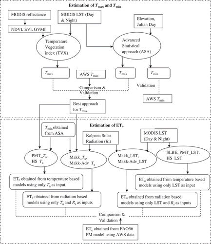
The main objective of this study is to obtain ET_o at high spatio-temporal resolution using limited weather variables. Therefore, performance evaluation of radiation-based (Makkink and Makkink-Advection), temperature-based (Hargreaves-Samani, HS), simple LST-based equation (SLBE), and Penman-Monteith temperature (PMT) models was carried out with the FAO56-PM method. For these ET_o models, minimum T_a (T_min) and maximum T_a (T_max) are crucial parameters. The quality of T_a data influences the ET_o values. Hence, comparison of the advanced statistical (ASA) and TVX approaches for estimation of T_max and T_min was conducted. Furthermore, LST was replaced by T_a in the ET_o models to check its pertinence. Comparison between ET_o values estimated by employing the above-mentioned ET_o models using LST and T_a (obtained from the best approach among TVX and ASA) as inputs was carried out. A schematic representation of these procedures is provided in Figure 1.

Figure 1. Schematic representation of methodology.

2 Study area

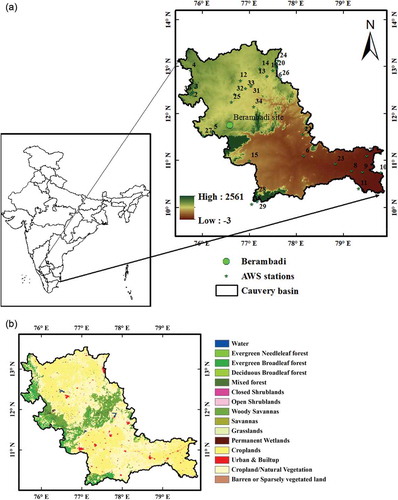
The Cauvery River is one of the major rivers of peninsular India and the river basin extends between 10°05′–13°30′N and 75°30′–79°45′E. The River basin covers an area of 81 155 km² and lies in the states of Karnataka, Kerala, Tamil Nadu and Pondicherry. It is one of the largest rivers of southern India and depends heavily on monsoon rains; hence it is prone to droughts when the monsoon fails. There is a serious conflict between Karnataka and Tamil Nadu states on the issue of sharing the river water. Due to this, accurate water management has become essential. In terms of physiography, the basin can be divided into three parts: the Western Ghats area, the Plateau of Mysore and the Delta area (CWC and NRSC (Central Water Commission and National Remote Sensing Centre) 2014). The Delta forms the lower part of the Cauvery basin and is the most fertile tract, while the Western Ghats consists of a mountainous region and runs parallel to the western coast (Fig. 2(a)). The mean T_max and T_min are 34.31 and 17.15°C, respectively, for the period 1969–2004 (http://www.india-wris.nrsc.gov.in). Precipitation varies substantially over the basin; while the western part of the basin receives the southwest monsoon (June–September), the northeast monsoon (October–December) serves the eastern part. The rainfall during other periods is insignificant. The basin receives mean annual precipitation of about 1075 mm/year. Annual rainfall (1970–2004) varies from 1700 to 3800 mm/year in the Western Ghats and 600 to 800 mm/year in the Plateau of Mysore, while the Delta area receives 500–1000 mm/year (www.india-wris.nrsc.gov.in). Land use/land cover of the basin is broadly classified as agricultural, non-agricultural, forest and habitation land. Data for the year 2012 show more than 60% of the land in the Cauvery basin is cultivable, 1.15% is urban/built-up, 17.91% is forest regions and the remainder is non-cultivable. Finger millet and paddy are the principal crops of the Mysore Plateau and Delta regions, respectively.

Figure 2. (a) Location of the study area with the automatic weather stations and land cover types indicated by numbers. (Stations 1–5 belong to land cover class F, 6–14 – class C, 15–18 – class U/BP and 19–35 – class C/NV. (b) MODIS land use/land cover map of the study area showing location of the Berambadi site, details of land cover classes, and elevation of the study area. F: forest, C: croplands and U/B: urban/built-up, C/NV: croplands/natural vegetation.

3 Methodology

3.1 Data used and pre-processing

Data on T_max, T_min, relative humidity, wind speed and sunshine hours required for the estimation of ET_o using the FAO56-PM method were acquired from the automatic weather stations (AWS) installed by the Indian Space Research Organization (ISRO). A total of 35 AWSs located within the basin were considered in this study (Table 1). According to the Indian Council of Agricultural Research (ICAR), Cauvery basin comprises three agro-climatic zones, namely the southern plateau and hill region, the east coast plains and hill region, and the west coast plain and ghats region (Ghosh 1991). This categorization is based on soil type, climate, temperature and its variations, rainfall and other agro-meteorological characteristics, as well as water demand and supply characteristics, including quality of water and aquifer conditions. Available stations within the Cauvery basin were grouped into three climatic regions according to ICAR, namely semi-arid, semi-arid to humid, and humid. In addition, observed R_s data obtained from a pyranometer for the years 2013 and 2014 were collected for the Berambadi site, which is located in the Gundalpet taluk of Karnataka State (11.76°N; 76.58°E) at an altitude of 870 m a.s.l. (Fig. 2(a)). The LST (MYD11A1) and reflectance (MYD09GA) values of near-infrared (NIR), Red, Blue and SWIR2 data were obtained from the MODIS sensor of the Aqua satellite. Since 2002, MODIS has been carried on the NASA (US National Aeronautics and Space Administration) polar-orbiting Aqua satellite, which passes from south to north at about 01:30/13:30 h local solar time each day in sun-synchronous orbit. The MODIS sensor, with 36 bands, provides near-daily global coverage with high spatial resolution. Since the passing time of the satellite over the study region is in the afternoon, maximum LST can be seen during this time. Minimum LST occurs in the early morning. The difference between minimum LST and observed LST at around 02:00 h is the least. In this study, night-time LST refers to minimum LST and daytime LST refers to maximum LST; T_max and T_min measurements were selected corresponding to these. The R_s data were taken from the Kalpana-1 satellite, a geostationary satellite that was launched in 2002. It carries a Very High Resolution Radiometer (VHRR)/2 sensor and receives information from visible, infrared and thermal infrared bands at spatial resolutions of 2 km and 8 km. The MODIS LULC (MCD12Q1) product was used for segregating the LST pixels according to the International Geosphere Biosphere Programme (IGBP) classification (Friedl et al. 2010). Digital elevation data were obtained from the Shuttle Radar Topography Mission (SRTM). All the datasets considered are from the period 2012–2014. Details of the datasets used are provided in Table 2.

Table 1. Description of land cover types and climatic characteristics of automatic weather stations in Cauvery basin. Lat.: latitude; Lon.: longitude; LULC: land use/land cover, F: forest, C: croplands, U/B: urban/built-up area, C/NV: croplands/natural vegetation; H: humid, SA: semi-arid, SA-SH: semi-arid/sub-humid.

No.	Station ID (Location)	Lat.	Lon.	LULC	Climate
1	ISRO607_15F25F (Kover Colly Tea Estate, Somwaripet)	12.57	75.85	F	H
2	ISRO608_15F260 (Elk Hill Estates, TBBTCL, Sodapur)	12.48	75.79	F	H
3	ISRO611_15F263 (Kottoli Village, K. Boikeri, Virajpet)	12.46	75.80	F	SA-SH
4	ISRO323_15F143 (ICRI, RS, Donigal, Sakleshpur)	12.92	75.75	F	H
5	ISRO434_15F1B2 (RARS Ambalavayal Wayanad)	11.61	76.21	F	H
6	ISRO169_15F0A9 (VC&RI, Namakkal)	11.10	78.16	C	SA
7	ISRO177_15F0B1 (TNRRI, Aduthurai, Thanjavur Dist.)	11.10	79.5	C	SA-SH
8	ISRO181_15F0B5 (SWMRI, Kattuthottam, Thanjavur)	10.78	79.18	C	SA-SH
9	ISRO182_15F0B6 (KVK, Nidamangalam, Thiruvarur Dist.)	10.76	79.41	C	SA
10	ISRO183_15F0B7 (KVK, Sikkal Nagapattinam Dist.)	10.75	79.80	C	SA-SH
11	ISRO186_15F0BA (ARS, Nadimuthu Nagar, Pattukottai)	10.41	79.33	C	SA-SH
12	ISRO387_15F183 (HLBC Subdivision, Nagamangala)	12.71	76.81	C	SA
13	3 ISRO834_15F342 (Scientist silk farm breeding, KSSRDI Bidadi, Ramanagara)	12.80	77.38	C	SA
14	ISRO844_15F34C (Dy. Director Sericulture, Govt. silk farm (m) Magadi)	12.96	77.23	C	SA
15	ISRO178_15F0B2 (TNAU, Main Campus, Coimbatore)	11.00	77.00	U/B	SA-SH
16	ISRO222_15F0DE (LPSC ISRO, Banglore)	12.96	77.58	U/B	SA
17	ISRO223_15F0DF (ISRO HQ, Banglore)	13.03	77.57	U/B	SA
18	ISRO315_15F13B (HQ, TC, IAF, JC Nagar, Hebbal, Banglore)	13.01	77.57	U/B	SA
19	ISRO123_15F07B (RV College of Engineering, Bangalore)	12.92	77.50	C/NV	SA
20	ISRO124_15F07C (AICRP AGR, UAS GKVK, Bangalore)	13.08	77.57	C/NV	SA
21	ISRO170_15F0AA (HRS, Yercaud, Salem Dist.)	11.70	78.21	C/NV	SA-SH
22	ISRO172_15F0AC (KVK, Sandhiyur, Salem Dist.)	11.56	78.13	C/NV	SA-SH
23	ISRO179_15F0B3 (AEC&RI, Kumulur, Lalgudi, Trichy)	10.93	78.83	C/NV	SA
24	ISRO216_15F0D8 (AF Station, Yelahanka, Bangalore)	13.13	77.61	C/NV	SA
25	ISRO322_15F142 (CSRTI, Sorampura, Mysore)	12.25	76.62	C/NV	SA
26	ISRO325_15F145 (IIHR, Hessaraghatta lake post, Banglore)	12.75	77.66	C/NV	SA
27	ISRO435_15F1B3 (CVAS Pookot Lakkidi Wayanad)	11.53	76.02	C/NV	H
28	ISRO443_15F1BB (President MGO Marayoor Idukki)	10.27	77.16	C/NV	H
29	ISRO444_15F1BC (KDHPCPL Munnar Idukki)	10.14	77.17	C/NV	H
30	ISRO621_15F26D (Codagu Planters Association, GT Road, Madikeri)	12.42	75.75	C/NV	H
31	ISRO837_15F345 (Maddur)	12.59	77.04	C/NV	SA
32	ISRO838_15F346 (Sri Ranga Patnam)	12.42	76.69	C/NV	SA
33	ISRO839_15F347 (DD of Sericulture)	12.54	76.92	C/NV	SA
34	ISRO841_15F349 (Kollegala Mandal Sericulture)	12.15	77.09	C/NV	SA
35	ISRO995_15F3E3 (Anthoniar Colony Munnar)	10.08	77.05	C/NV	H

Table 2. Details of the datasets used. LST: land surface temperature (°C); R_s: solar radiation (MJ m⁻² d⁻¹).

Source	Parameter	Product name	Spatial resolution	Purpose
MODIS/Aqua	LST (day/night)	MYD11A1	1 km	Estimation of ETo and Ta (max/min)
VHRR(2)/Kalpana-1	Rs	-	2 km	Estimation of ETo
MODIS/Aqua	Reflectance values of NIR, Red, Blue and SWIR2 bands	MYD09GA	500 m	Estimation of vegetation indices
MODIS/Aqua	LULC	MCD12Q1	500 m	Segregation of ETo
SRTM	Elevation	-	90 m	Prediction of Ta (max/min) and ETo
AWS	RH (max/min), Ta (max/min), wind speed and sunshine hours	-	Point scale	Validation

The MODIS LST (day/night) projections were changed from sinusoidal to geographical projection by employing a nearest-neighbour method using the MODIS reprojection tool developed by NASA (Dwyer and Schmidt 2006). These were aggregated from 1 km to the Kalpana-1/VHRR data at a spatial resolution of 2 km by spatial averaging. Reflectance values of NIR, Red, Blue and SWIR2 spatial resolutions were aggregated from 500 m to 2 km using spatial averaging, and these were used to derive vegetation indices. The MODIS LULC data were upscaled from 500 m to 2 km, and later used to segregate the pixels based on the IGBP classification. The SRTM elevations used in the estimation of T_a (max/min) were aggregated from 90 m to 2 km.

3.2 Estimation of satellite-based air temperature

In this study ASA and TVX approaches were employed for T_a (max/min) estimation and the results were validated with T_a (max/min) obtained from the AWS.

3.2.1 Statistical approaches

Most of the statistics-based approaches developed are based on relating satellite-based LST (max/min) and auxiliary data as predictors, with T_a (max/min) obtained from meteorological stations as the predictand (Mostovoy et al. 2006, Cristobal et al. 2008, Fu et al. 2011, Benali. et al. 2012, Rhee and Jungho 2014, Xu et al. 2014, Zeng et al. 2015). In this study, different statistical approaches from simple (one predictor variable, LST) to multiple (more than one predictor) were tested. In addition to LST (day/night), other auxiliary variables such as elevation, latitude, longitude and Julian day were selected as predictors for the estimation of T_a (max/min). Out of 14 models developed by Benali. et al. (2012), eight were selected for analysis of their performance for the study region (Table 3). Benali. et al. (2012) used a mixed bootstrap method with jack-knife resampling; however, in this study, only the bootstrap technique was employed to generate samples, since sufficient observed T_a values obtained from the AWSs were available over the study region (Bai and Wei. 2008). The eight models were selected depending on the availability of data for the study region: 70% of the available data (for 2012 and 2013) was used for calibration and the remaining 30% for validation of the models, and these datasets were employed in the generation of respective calibration and validation of 1000 bootstrap samples. The Levenberg-Marquardt algorithm was employed to minimize the square of the absolute differences between predictions and observations. The obtained coefficients were later applied to estimate T_max and T_min from the validation datasets. The statistical relationship between estimated T_max/T_min and observed T_max/T_min was quantitatively evaluated by computing statistical error indices. Information about the statistical error indices employed is given in Section 3.4.

Table 3. Goodness-of-fit indicators computed between T_a values obtained from eight models and from AWSs. r: Pearson correlation coefficient; RMSE: root mean square error; NSE: Nash-Sutcliffe efficiency; a to e: model coefficients (see Appendix 3 for values used in ASA); LST_day: daytime land surface temperature, LST_night: night-time land surface temperature; peak and phase are coefficients of the cosine function; JD: Julian day; ele: elevation.

Model no.	Model equation	Tmax			Tmin
		r	RMSE	NSE	r	RMSE	NSE
1	aLSTday + b	0.75	2.71	0.55	0.57	3.44	0.32
2	aLSTnight + b	0.74	2.75	0.53	0.84	2.29	0.69
3	aLSTday + bLSTnight + c	0.82	2.32	0.67	0.84	2.25	0.71
4		0.74	2.74	0.54	0.58	3.43	0.32
5		0.74	2.75	0.54	0.84	2.30	0.69
6		0.82	3.22	0.36	0.84	2.33	0.68
7		0.73	2.79	0.52	0.62	3.31	0.37
8		0.83	2.29	0.68	0.83	2.34	0.68

3.2.2 Temperature–vegetation index (TVX) approach

Prihodko and Goward (1997) proposed a contextual method by fitting a linear relationship between spectral vegetation index (VI) and LST. Estimation of T_max is based on the assumption that the bulk temperature of an infinitely thick vegetation canopy is close to the ambient air temperature. Several authors have applied the TVX method to check the potential of the method for various climatic regions using data from different sensors (Stisen et al. 2007, Vancutsem et al. 2010, Nieto et al. 2011, Shah et al. 2013, Wenbin et al. 2013). Nevertheless, the mandatory negative linear relationship between the normalized difference vegetation index (NDVI) and LST is difficult to attain in several conditions due to the influence of seasonality, ecosystem type and soil moisture variability (Benali. et al. 2012). Thus, T_max was calculated by applying maximum VI (VI_max) from a simple linear equation, which was obtained by ascertaining the linear relationship between LST and VI. In the past, only NDVI has been considered for T_max estimation (Prihodko and Goward 1997, Stisen et al. 2007, Vancutsem et al. 2010, Nieto et al. 2011). Conventional NDVI is saturated when leaf area index > 3.5 and this can be avoided by employing the enhanced VI (EVI) and global vegetation moisture index (GVMI) (Le Naire et al. 2006, Guerschman et al. 2009). The GVMI is asymptotically linked to equivalent water thickness (Guerschman et al. 2009) and the presence of vegetation moisture influences the variations in T_a. Here, an attempt is made to examine the potential of two other vegetation indices, namely EVI and GVMI, in estimating T_max. The accuracy of this approach depends on two important points. Firstly, there should be a strict negative relationship between LST and VI and, secondly, the value of VI_max, since the assumption of this approach is that LST is of thick vegetation, is close to T_a. Many researchers have considered different values of maximum NDVI depending on their study region, and this varied from 0.65 to 0.90 (Prihodko and Goward 1997, Stisen et al. 2007, Vancutsem et al. 2010, Wenbin et al. 2013). In this study, maximum values of NDVI (NDVI_max), EVI (EVI_max) and GVMI (GVMI_max) varied between 0.40 and 0.90 for the various land cover classes individually in the estimation of T_max for the study region.

(1)

(2)

(3)

where NIR, RED, BLUE, SWIR2 are the reflectances of their respective bands. In this study, the values of G, C₁, C₂ and L in the EVI equation (Equation (2)), which account for aerosol scattering and absorption (Guerschman et al. 2009), are 2.5, 6.0, 7.5 and 1.0, respectively.

3.3 Reference evapotranspiration models

Reference evapotranspiration (ET_o) is “the rate of evapotranspiration from a hypothetical reference crop with an assumed crop height of 0.12 m, a fixed surface resistance of 70 sec m⁻¹ and albedo of 0.23, closely resembling the evapotranspiration from an extensive surface of green grass of uniform height, actively growing, well watered and completely shading the ground” (Allen et al. 1998, McMahon et al. 2013, Pereira et al. 2015). The standardized reference evapotranspiration equation can be expressed as (McMahon et al. 2013):

(4)

where ET_o is the daily reference crop evapotranspiration (mm d⁻¹), T_mean is the mean daily T_a (°C) at 2 m, u₂ is the average daily wind speed (m s⁻¹) at 2 m, R_n is the net daily radiation (MJ m⁻² d⁻¹), G is the soil heat flux (MJ m⁻² d⁻¹), e_s − e_a is the vapour pressure deficit (kPa), γ is the psychometric constant (kPa °C⁻¹) and Δ is the slope of the saturation vapour pressure curve (kPa °C⁻¹). In this study, the FAO56-PM equation was applied to estimate ET_o at the point scale by applying data of AWSs as inputs. These results were then used for validation of ET_o obtained using satellite-based approaches (details are given in the following sections).

3.3.1 Radiation-based models

In 1957, Makkink proposed a radiation-based formula by modifying the Penman equation which requires only R_s and T_a data (Arellano and Irmak 2016). De Bruin (1987) further simplified the Makkink equation to estimate ET_o accurately under non-water stress conditions (Cruz-Blanco et al. 2014b), which can be expressed as:

(5)

where is a simplification parameter, which varies from 0.63 to 0.90 for different climatic conditions (De Bruin 1987, De Bruin et al. 2010, Stewart et al. 1999, Schuttemeyer et al. 2007, Bois et al. 2008, Cammalleri and Ciraolo 2013), R_s is solar radiation. and the other parameters are as explained in Section 3.3. De Bruin et al. (2012b) introduced the advection-based revised Makkink equation by accounting for advection effects under semi-arid conditions, which can be expressed as:

(6)

3.3.2 Temperature-based models

In the absence of radiation measurements, the simplified temperature models work better in semi-arid and arid climates, as reported by Verhoef and Feddes (cited from Di Stefano and Ferro 1997). These models require only T_a or LST data for the estimation of ET_o. Many temperature-based models are available and they have been successfully applied worldwide (e.g. Thornthwaite 1945, McCloud 1955, Hamon 1961, Blaney and Criddle 1962, Hargreaves and Samani 1985). In most cases, the Hargreaves-Samani (HS) equation performed better than other models (Di Stefano and Ferro 1997, Gavilan et al. 2006, Aguilar and Polo 2011, Maeda et al. 2011, Todorovic. and Pereira 2013, Kisi 2014, Almorox et al. 2015). Hence, in this study, the HS model was selected among the available empirical temperature-based equations.

3.3.2.1 The Hargreaves-Samani (HS) equation

The HS equation is an empirical equation and requires only T_mean, T_max, T_min and extraterrestrial radiation (R_a) for derivation of ET_o. This equation tends to overestimate in humid climates, since it requires only T_a data and varies with it, therefore requiring regional calibration for better performance. The HS equation can be written as:

(7)

where R_a is extraterrestrial solar radiation (MJ m⁻² d⁻¹) and C_H is the Hargreaves empirical coefficient, set to 0.0023 for arid and semi-arid regions.

3.3.2.2 The Penman-Monteith temperature (PMT) model

The inputs required in the FAO56-PM equation for ET_o estimation are R_n, e_s − e_a and u₂, and these may be estimated by employing alternative methods, which use only T_max and T_min, in the case of non-availability of other climatic variables over the study region. This approach is known as the Penman-Monteith temperature (PMT) model (Todorovic. and Pereira 2013, Raziei and Pereira 2013a). In this study, the procedures evolved by Todorovic and Pereira (2013) and Raziei and Pereira (2013a) were followed to estimate the parameters R_n, e_s − e_a and u₂, and these were then employed in the FAO56-PM equation (Equation (4)) to derive ET_o for the Cauvery basin. The method is elaborated in Appendix 1.

3.3.2.3 The simple LST-based equation (SLBE)

Rivas and Caselles (2004) proposed a new simplified equation for estimation of ET_o with LST and local standard meteorological data.

(8)

where LST is land surface temperature obtained from satellite data. The parameters a and b depend on the local meteorological data, obtained by segregating the PM equation into a radiation term and an aerodynamic term, and these can be expressed as:

(9)

(10)

where ε_s is the emissivity of the surface, σ is the Stefan-Boltzmann constant (4.9 × 10⁻⁹ MJ m⁻² K⁻⁴ d⁻¹), r_c is the crop canopy resistance (s m⁻¹), r_a is the aerodynamic resistance (s m⁻¹), α is the albedo of the surface, and the other parameters are as elaborated previously.

In this study, in place of T_a data, LST values were employed in the HS (HS_LST), PMT (PMT_LST) and Makkink (Makk_LST) models. As mentioned in Section 3.2, the best T_a values obtained between the two approaches were employed in the HS (HS_T_a), PMT (PMT_T_a), simple Makkink (Makk_T_a) and advection-revised Makkink (Makk_adv_T_a) equations.

3.4 Performance evaluation indices

Estimated T_max and T_min were validated with observed T_max and T_min values obtained from the AWSs. Furthermore, ET_o estimated using temperature- and radiation-based methods was evaluated with ET_o calculated using the FAO56-PM model at the AWSs (referred to herein as observed values). The Pearson correlation coefficient (r) was used to measure the correlation between the estimated and observed values. The value of r varies from −1 to +1, where 0 indicates no correlation and ±1 high correlation. The Nash-Sutcliffe efficiency criterion (NSE; Nash and Sutcliffe 1970) varies from −∞ to 1. An efficiency of 1 represents a perfect match between estimated and observed values and 0 indicates that the estimated values are equal to the mean of the observed values. Negative NSE indicates that the observed mean is better than the estimated values. This is sensitive to means and variances of the differences found between the observed and estimated values. Root mean square error (RMSE) is one of the commonly used error indices. Lower RMSE indicates better performance of the model (Moriasi et al. 2007). Mean absolute percentage error (MAPE) is a measure of prediction accuracy. Mean bias error (MBE) is the average difference between the estimated and observed values. The equations for calculating these goodness-of-fit indicators are given in Appendix 2.

4 Results and discussion

4.1 Estimation of satellite-based air temperature

The values of T_max and T_min were estimated using ASA and TVX approaches (as described in Section 3.2). These estimated T_max and T_min were validated with the corresponding AWS T_a data. The performance of the selected methodologies was analysed by considering data of all the stations using the statistical error indices r, RMSE and NSE. The better T_max results obtained among the mentioned approaches and T_min were utilized in the estimation of ET_o.

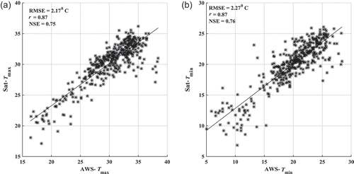
The error indices of both T_max and T_min obtained by the eight models are given in Table 3. The results indicate that, of these, Models 3 and 8 performed best, with high r values of 0.84 and 0.83, NSE of 0.71 and 0.68, and low RMSE of 2.25 and 2.29°C, respectively. Together, LST_day and LST_night could explain 82 and 84% of variability in T_max and T_min, respectively. This indicates a strong relationship between LST and T_a. The addition of Julian day and elevation into the model increased the accuracy in T_max estimation, but did not improve accuracy in T_min estimation. Coefficients of the considered models (for the estimation of T_max and T_min) are provided in Appendix 3. Scatterplots between predicted T_max, T_min (obtained from the best models) and observed T_max, T_min for the year 2014 are shown in Figure 3. The results in Figure 3 indicate that Model 3 and Model 8 (Table 3) estimated T_min and T_max more accurately (r, RMSE and NSE of 0.87, 2.27°C and 0.76, and 0.87, 2.17°C and 0.75, respectively) .

Figure 3. Scatter plots between predicted and observed (a) T_max and (b) T_min.

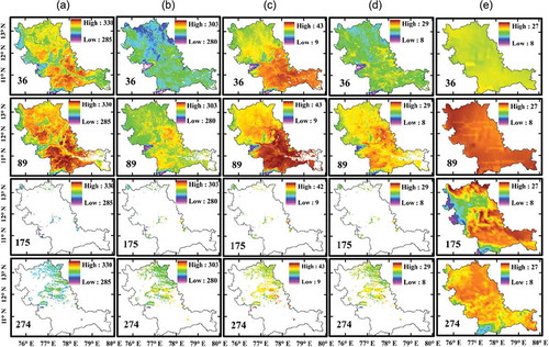
Spatial variations of T_max and T_min for the year 2014 representing different seasons are shown in Figure 4(c) and (d). The Western Ghats have low T_max and T_min compared to other regions. This is due to higher elevation and forest cover. Summer season (DOY 89) has higher T_max and T_min than other seasons. One of the disadvantages of using satellite data is the presence of cloud cover causing gaps in the datasets, represented by white, as may be seen in Figure 4(c) and (d). The accuracy of T_max and T_min estimation depends on the quality of the LST product and the satellite passing time. In this study, the Aqua satellite LST product was used, which improves the T_min estimation compared to other satellites, as its passing time is closer to the time of T_min.

Figure 4. Spatial distributions of (a) LST_day (K), (b) LST_night (K), (c) T_max (°C), (d) T_min (°C), and (e) R_s (MJ m⁻² d⁻¹) on days 36, 89, 175 and 274 of the year 2014, representing different seasons.

The T_max was estimated using the TVX approach by varying the maximum values of the three vegetation indices NDVI, EVI and GVMI (Equations (1)–(3)). Statistical analysis was performed between these estimated T_max values and the observed T_max, and the results are depicted in Figure 5. Scatter plots between estimated T_max using the best maximum vegetation index and observed T_max for forest (F), croplands (C) and croplands/natural vegetation (C/NV) land cover classes are shown in Figure 5(1). Maximum vegetation index values for the considered land cover classes were selected individually depending on the accuracy of T_max estimation. Accuracy was adjudicated based on RMSE and r, and these were computed for the F, C and C/NV land cover classes by varying the maximum vegetation index values from 0.9 to 0.4, with an interval of 0.05 (Fig. 5(2)).

Figure 5. (1) Scatter plots between predicted T_max and AWS T_max; and (2) variations of RMSE and r values obtained between predicted T_max and AWS T_max for varying VI_max for (a) forest, (b) croplands, and (c) croplands/natural vegetation land cover classes.

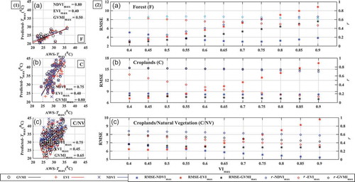
As the NDVI_max was reduced for the forest class, RMSE decreased from 3.84 to 3.01°C at NDVI_max = 0.8 and, after this, began to increase from 3.12 to 5.10°C. However, r gradually decayed from 0.66 to 0.12 as NDVI_max was reduced (Fig. 5(2,a)). In the case of the croplands class, RMSE showed less variation for different NDVI_max values and RMSE was lowest at NDVI_max = 0.75, and r values gradually increased from 0.70 to 0.78 as NDVI_max was decreased (Fig. 5(2,b)). For the C/NV class, RMSE and r gradually increased from 5.25 to 6.84°C and 0.58 to 0.68, respectively, and an optimal value of NDVI_max = 0.75 was selected (Fig. 5(2,c)). Thus, NDVI_max values of 0.8, 0.75 and 0.75 were selected for F, C and C/NV classes, respectively. At these NDVI_max values, r and RMSE between estimated T_max and observed T_max were found to be 0.63 and 3.19°C, 0.72 and 8.15°C, and 0.60 and 5.44°C for F, C, C/NV classes, respectively (Fig. 5(1,a–c)).

For the EVI, as the EVI_max was reduced from 0.9 to 0.4 for the forest class, RMSE decreased from 10.84 to 3.01°C and r increased from 0.47 to 0.64 (Fig. 5(2,a)). However, for the croplands class, RMSE abruptly decreased from 16.63 to 7.13°C and r increased from 0.14 to 0.63 (Fig. 5(2,b)). In the case of croplands/natural vegetation, RMSE reduced from 9.81 to 6.22°C and r increased from 0.34 to 0.60 (Fig. 5(2,c)). Therefore, optimal EVI_max values of 0.4, 0.4 and 0.45 were selected for F, C and C/NV classes, respectively. At these values of EVI_max, r and RMSE between estimated T_max and observed T_max were calculated as 0.63 and 3.47°C, 0.55 and 7.30°C, and 0.57 and 6.14°C for F, C and C/NV classes, respectively (Fig. 5(1,a,b,c)).

As the value of GVMI_max was reduced from 0.9 to 0.4, for the forest land cover class, RMSE gradually decreased from 7.60 to 2.85°C and r increased from 0.62 to 0.67 to a level of GVMI_max = 0.55, and eventually decreased to 0.60 (Fig. 5(2,a)). For the croplands class, RMSE and r gradually increased from 6.98 to 8.03°C and from 0.74 to 0.78, respectively (Fig. 5(2,b)). In the case of croplands/natural vegetation, the improvement in RMSE values, even after gradual reduction in GVMI_max, was small, whereas r showed a gradual increase from 0.43 to 0.61 (Fig. 5(2,c)). Therefore, the optimal values of GVMI_max of 0.5, 0.8 and 0.65 were selected for F, C and C/NV classes, respectively. At these values of GVMI_max, r and RMSE between estimated T_max and observed T_max were calculated as 0.67 and 3.39°C, 0.77 and 7.67°C, and 0.56 and 6.64°C, for F, C and C/NV classes, respectively (Fig. 5(1,a–c)). Among the vegetation indices considered, GVMI predicted better T_max for the F and C land cover classes compared to EVI and traditional NDVI vegetation indices for the study region, but no notable improvement was seen. This indicates that moisture content of vegetation influences T_max more than the density of vegetation. The GVMI represents vegetation moisture content, whereas EVI and NDVI represent density of vegetation; therefore, GVMI performed better than EVI and NDVI. However, the TVX method yielded poor r with high RMSE values for the considered optical vegetation indices, compared to the ASA. Hence T_max and T_min values obtained using the ASA approach were used for the estimation of ET_o.

4.2 Validation of satellite-based solar radiation

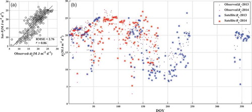
Solar radiation (R_s) values obtained from the Kalpana-1 satellite were evaluated with the observed data, to assess the potential of their application for the estimation of ET_o. Observed R_s data were available only for Berambadi station, located in the croplands land cover class, for the years 2013 and 2014. Therefore, analysis was only performed for the croplands class. Linear regression between the AWS and satellite R_s values generated a slope of 0.68 (RMSE = 2.76 MJ m⁻² d⁻¹, r = 0.86) (Fig. 6(a)). Temporal patterns of the satellite R_s (Sat-R_s) data for both years were analysed; the statistical analysis indicated that Sat-R_s corresponded well with the observed R_s, with RMSE = 2.87 MJ m⁻² d⁻¹, r = 0.88 for 2013 and RMSE = 2.63 MJ m⁻² d⁻¹, r = 0.79 for 2014, as shown in Figure 6(b). This shows that Sat-R_s can be applied in radiation-based models over the Cauvery basin, as it is mostly covered by croplands. However, underestimation of Sat-R_s was found for the years 2013 and 2014, with relative RMSE values of 18.66 and 15.84, respectively.

Figure 6. (a) Scatter plot between satellite and observed R_s values and (b) temporal variations of satellite and observed R_s for the years 2013 and 2014.

Spatial variation in Sat-R_s for 2014, representing different seasons, is shown in Figure 4(e), illustrating that R_s values are smaller for the winter season (DOY 36), with very small spatial variation, whereas for the summer (DOY 89) they are greater than in other seasons, with less spatial variation for all land cover classes. In the case of the monsoon (DOY 175) and post-monsoon (DOY 274) seasons, R_s values are smaller for the Western Ghats region than for the other regions. During the monsoon season, the upper part of the basin has smaller R_s than the lower part because of the southwest monsoon. In contrast, during the post-monsoon season, the upper part of the basin has higher R_s than the lower part of the basin due to the northeast monsoon (Fig. 4(e)). During the monsoon and post-monsoon seasons, estimation of R_s is difficult because of the presence of dense clouds.

4.3 Evaluation of ET_o models

The considered LST- and T_a-based temperature (SLBE, HS, PMT) and radiation (Makk, Makk_adv) ET_o models were compared with the FAO56-PM ET_o estimated using AWS data at the point scale. Analysis of the estimated ET_o using satellite data was carried out separately by considering different land cover classes of the study region with various climatic conditions.

4.3.1 Statistical evaluation of ET_o for different land cover classes

The data for the years 2012, 2013 and 2014 were used to estimate ET_o by the temperature- and radiation-based models at 2 km spatial resolution. The ET_o values estimated using different datasets were segregated based on MODIS LULC data to assess the ET_o for various land cover classes. Based on the availability of satellite and AWS data, the analysis was performed for three land cover classes, namely forest, croplands and croplands/natural vegetation. Scatter plots between LST-based and AWS ET_o and between T_a-based and AWS ET_o for different land cover classes are presented in Figures 7 and 8, respectively. Initially, LST was employed in temperature- and radiation-based ET_o models instead of T_a, to examine the adoptability of LST data. Thereafter, T_max and T_min estimated using the ASA from LST_day and LST_night with auxiliary variables were applied in the ET_o models. The performance of these LST- and T_a-based temperature- and radiation-based ET_o models was assessed through the goodness-of-fit indicators RMSE (mm d⁻¹), r, MAPE (%) and MBE (mm d⁻¹) for the considered land cover classes. The statistical results imply that the LST-based SLBE model underestimated ET_o for forest, croplands and croplands/natural vegetation classes (F: RMSE = 1.06, r = 0.53, MAPE = 23.98 and MBE = 0.92; C: RMSE = 0.42, r = 0.77, MAPE = 8.42 and MBE = 0.25; and C/NV: RMSE = 1.06, r = 0.73, MAPE = 18.38 and MBE = 0.64) (Fig. 7(a)). The HS_LST, PMT_LST and Makk_LST models predominantly overestimated ET_o for F, C and C/NV land cover classes (Fig. 7(b)–(d)). Among the considered LST-based ET_o models, SLBE satisfactorily predicted ET_o with smaller RMSE and MAPE for the considered land cover classes because (a) aerodynamic and (b) radiation terms in this equation were obtained using local weather station data, and these were applied for the entire basin. The HS_LST and PMT_LST methods depend solely on LST data; hence the ET_o values were found to be higher than the FAO56-PM ET_o, and this is due to higher LST than T_a over the study region. Nevertheless HS_LST and PMT_LST yielded high r values for the forest class. Statistical error indices showed that the Makk_LST model yielded better ET_o values than the HS_LST and PMT_LST models because R_s data were utilized along with LST.

Figure 7. Scatter plots between estimated ET_o using different LST-based ET_o models from satellite data (Sat-LST-ET_o) and ET_o values obtained from the FAO56-PM model using observed AWS data (AWS-ET_o) for forest, croplands and croplands/natural vegetation.

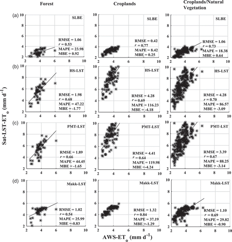
Figure 8. Scatterplots between estimated ET_o using different T_a-based ET_o models from satellite data (Sat-T_a-ET_o) and ET_o values obtained from FAO56-PM using observed AWS data (AWS-ET_o) for forest, croplands and croplands/natural vegetation.

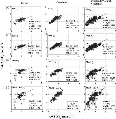
Figure 8 illustrates the goodness-of-fit indicators computed by evaluating T_a-based radiation- and temperature-based ET_o models with PM ET_o. Compared to LST-based ET_o models, T_a-based models, such as HS_T_a, PMT_T_a, Makk_T_a and Makk-adv_T_a models, gave satisfactory ET_o values for all the land cover classes with smaller RMSE, MAPE and MBE (Fig. 8). High r values were observed for all land cover classes for all T_a-based ET_o models except for the Makk_T_a and Makk-adv_T_a equations for the forest class. This may be due to insufficient weather variables required to estimate ET_o. And also Sat_R_s data used in these two equations needed evaluation for the forest class. T_max and T_min were estimated using the ASA approach by minimizing errors between LST_day/LST_night and T_max/T_min, which resulted in better performance of the T_a-based ET_o models. For the HS_T_a model, RMSE, MAPE and r ranged from, respectively, 0.77, 19.86 and 0.71 for forest to 1.14, 31.83 and 0.86 for croplands, with a mean bias of −0.87 (Fig. 8(a)). The PMT_T_a model yielded RMSE, MAPE and r values ranging, respectively, from 0.61, 14.93 and 0.71 for forest to 0.98, 27.24 and 0.84 for croplands, with a mean bias of −0.69 (Fig. 8(b)). In contrast, the Makk_T_a (Makk-adv_T_a) models gave RMSE values ranging from 0.95 (1.77) for C/NV to 1.08 (2.06) for croplands, with r in the range 0.49 (0.54) for forest to 0.85 (0.87) for croplands, and MAPE in the range 24.92 (47.85) for forest to 30.42 (57.72) for croplands, with a mean bias of −1.15 (−1.78) (Fig. 8(c) and (d)). Overall, the statistical error indices imply that the PMT_T_a model performed slightly better than other ET_o models for all considered land cover classes. However, for the croplands class, the SLBE ranked first and the PMT_T_a model ranked second by more accurately predicting ET_o values than other LST- and T_a-based ET_o models (Table 4). Considering the overall results, the PMT_T_a ET_o model performed better, followed by the SLBE, HS_T_a and Makk_T_a, in that order.

Table 4. Ranking of ET_o models depending on the selected goodness-of-fit indicators obtained between ET_o_LST, and ET_o_T_a model-based estimates and FAO56 PM ET_o. SLBE: simple LST-based equation; PMT: Penman-Monteith temperature; HS: Hargreaves-Samani; Makk-adv: Makkink-Advection.

Model	Land use/land cover
	Forest	Croplands	Croplands/natural vegetation
SLBE	3	1	2
HS_LST	7	7	7
PMT_LST	6	8	8
Makkink_LST	5	5	5
HS_Ta	2	4	2
PMT_Ta	1	2	1
Makkink_Ta	4	3	3
Makk-adv_Ta	8	6	6

4.3.2 Statistical evaluation of ET_o for different climatic regions

In order to examine the performance of LST- and T_a-based ET_o models, the data for all available stations were grouped into three climatic regions according to ICAR, namely semi-arid, semi-arid to sub-humid, and humid. The climatic characteristic of each station are given in Table 1. According to the statistical analysis, for the semi-arid climate the SLBE performed slightly better than the other ET_o models (Table 5). This is because more of the meteorological stations considered for parameterization of aerodynamic and radiation terms have semi-arid climates, hence better ET_o values were estimated. The value of r was higher for the PMT_T_a model than the SLBE, implying that PMT_T_a can also perform better in semi-arid regions, as indicated in Table 5. Apart from the SLBE model, the other LST-based ET_o models provided poor estimates of ET_o, with higher RMSE values. In semi-arid to sub-humid climates, PMT_T_a ranked first, while HS_T_a and Makk_T_a ranked second and third, respectively, and the performance indices indicate satisfactory results of ET_o models under semi-arid to sub-humid climate (Table 5). Similar results were obtained for humid climates, with smaller RMSE, MAPE and MBE values for the PMT_T_a model, but slightly higher r values for the HS_T_a model than PMT_T_a and other ET_o models. In both the semi-arid to sub-humid and humid climates, considering the effect of air humidity, using T_dew instead of T_a and considering the effect of wind speed in PMT_T_a yielded better ET_o values. Overall, statistical analysis considering climatic characteristics suggested that the PMT_T_a model would more often estimate ET_o better than the other ET_o models in comparison with the FAO56-PM ET_o estimates, as indicated consistently with smaller RMSE, MAPE and MBE relative to those of the HS_T_a and Makk_T_a models, which ranked second and third, respectively. It is noteworthy that, in all climates, r values for the PMT_T_a model were slightly low compared to the HS_T_a model. Among the LST-based ET_o models, the SLBE performed better than the other models. The LST-based HS and PMT models consistently overestimated ET_o across all climatic regions relative to the other T_a- and LST-based ET_o models.

Table 5. Statistical analysis of LST- and T_a-based ET_o models for semi-arid, semi-arid to sub-humid, and humid climates. RMSE (mm d⁻¹): root mean square error; r: Pearson correlation coefficient; MAPE: mean absolute percentage error; MBE: mean bias error. See Table 4 for model abbreviations. Bold indicates best performing models.

ETo model	RMSE	r	MAPE	MBE	Rank
Semi-arid
SLBE_LST	0.64	0.59	12.18	0.42	1
HS_LST	3.81	0.54	99.93	–3.62	5
PMT_LST	3.89	0.50	101.71	–3.68	6
Makk_LST	1.21	0.62	32.25	–1.10	3
HS_Ta	1.06	0.68	27.85	–0.96	2
PMT_Ta	0.90	0.67	23.44	–0.78	1
Makk_Ta	1.02	0.62	26.89	–0.89	2
Makk-adv_Ta	1.98	0.65	53.40	–1.89	4
Semi-arid to sub-humid
SLBE_LST	0.84	0.60	17.89	0.70	4
HS_LST	2.86	0.66	64.85	–2.57	8
PMT_LST	2.84	0.64	63.43	–2.50	7
Makk_LST	0.95	0.75	23.28	–0.85	5
HS_Ta	0.76	0.77	18.47	–0.70	2
PMT_Ta	0.58	0.75	13.14	–0.48	1
Makk_Ta	0.84	0.71	20.73	–0.74	3
Makk-adv_Ta	1.91	0.75	47.45	–1.84	6
Humid
SLBE_LST	1.14	0.71	33.49	1.04	3
HS_LST	2.12	0.48	62.49	–1.85	7
PMT_LST	2.19	0.40	64.38	–1.88	8
Makk_LST	1.17	0.56	35.74	–0.77	5
HS_Ta	0.94	0.76	29.84	–0.84	2
PMT_Ta	0.88	0.74	27.91	–0.76	1
Makk_Ta	1.12	0.56	34.66	–0.74	4
Makk-adv_Ta	1.58	0.62	46.95	–1.21	6

4.3.3 Spatial and temporal analysis of ET_o models

Figure 9 illustrates the spatial distribution of estimated ET_o using LST- and T_a-based ET_o models for various days of the year (DOY: 36, 89, 175 and 274), representing winter, summer, rainy season and post-monsoon season, respectively. All ET_o models yielded low ET_o over the Western Ghats and high ET_o in the croplands and croplands/natural vegetation land cover classes, as shown in Figure 9. The Western Ghats area is covered with forest, has higher elevation and humid climates and this resulted in lower ET_o estimates from the considered ET_o models. Most of the C and C/NV land classes are at lower elevations with semi-arid climates and therefore higher ET_o was observed for all the ET_o models. The LST-based ET_o models – HS_LST and PMT_LST – predominantly overestimated ET_o for all land cover classes and for all climatic regions, as shown by the statistical analysis. The next two models – Makk_LST and Makk_adv_T_a – consistently overestimated ET_o over the study region. The SLBE model slightly underestimated ET_o for all land cover classes compared to the other ET_o models.

Figure 9. Spatial variation of ET_o obtained from the LST- and T_a-based models for days 36, 89, 175 and 274 of the year 2014, representing different seasons.

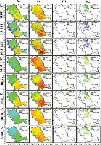
For the summer season, larger ET_o estimates were obtained and smaller ET_o values were observed for the rainy season for all ET_o models. Due to the presence of clouds, thermal sensors failed to provide LST data and hence T_max, T_min and ET_o values could not be estimated for cloudy pixels, as indicated by white in Figures 4 and 9. Therefore, for the monsoon and post-monsoon seasons, it was hard to evaluate the spatial distribution of ET_o. The ET_o obtained for the lower part of the Cauvery basin was higher than that for the upper part and this was observed for all ET_o estimates from the considered models (Fig. 9). The ET_o values ranged from 0.5 to 5.0 mm d⁻¹ for the SLBE model, being a slight underestimation of observed ET_o, whereas, for the T_a-based HS and PMT models, ET_o values ranged from 0.5 to 8.0 mm d⁻¹, showing slightly better spatial patterns than the other ET_o models. Similarly, estimates by T_a- and LST-based Makkink models ranged from 2.5 to 6.0 mm d⁻¹, showing less spatial variation across the study region.

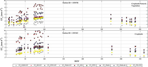
Furthermore, ET_o values estimated using LST- and T_a-based ET_o models were temporally evaluated with the FAO56-PM ET_o computed using AWS data. Temporal variations in ET_o obtained from the ET_o models considered are shown in Figure 10 for stations 15F07B and 15F34C, which belong to the C/NV and C land classes, respectively. According to Figure 10, the PMT_LST and HS_LST models overestimated ET_o compared to the Makk_LST and SLBE models for both C and C/NV land cover classes. Among the ET_o models considered, PMT_T_a, HS_T_a and Makk_T_a performed better than the other ET_o models for croplands (croplands/natural vegetation) land cover classes, with r, RMSE (mm d⁻¹), MAPE and MBE (mm d⁻¹) of 0.89 (0.91), 0.37 (1.03), 8.01 (29.47) and −0.19 (−1.01), and 0.90 (0.92), 0.46 (1.18), 10.25 (33.97) and −0.35 (−1.17), and 0.71 (0.87), 0.60 (1.06), 12.28 (30.12) and −0.32 (−1.03), respectively, as shown in Figure 10.

Figure 10. Temporal variation of ET_o obtained from satellite data and ET_o obtained from the FAO56-PM method for stations belonging to croplands/natural vegetation and croplands land cover classes. Gaps in the ET_o values are due to non-availability of LST, R_s and AWS data.

The accuracy of ET_o estimation depends on the quality of the input data. Hence, it is necessary to check the quality of input data before application in ET_o models. Satellite-based ET_o models depend on the quality of LST data. In this study, LST data were used for both T_a and ET_o estimation. The use of T_a estimated from satellite data, rather than direct LST data, in the ET_o estimations could increase the accuracy of ET_o calculation and this has been amply proven in this study. Overall, statistical and spatial analysis showed that the PMT_T_a model gave slightly better accuracy of ET_o estimates relative to the HS_T_a, Makk_T_a and SLBE models, and each of these four ET_o models performed better than other ET_o models considered in this study.

5 Summary and conclusions

In this study, air temperature (T_a) was estimated using remote sensing-based temperature–vegetation index (TVX) and the advanced statistical approach (ASA) and the results were validated with automatic weather station (AWS) T_a data. In the TVX approach, the relationship between different vegetation indices (NDVI, EVI and GVMI) and land surface temperature (LST) was examined by varying the maximum vegetation index values to estimate the maximum T_a (T_max) for the study region. The GVMI-based TVX approach performed better than the other vegetation index methods for the estimation of T_max. The ASA was used to estimate both T_max and T_min. In this approach, a bootstrap technique was employed to generate calibration and validation samples. The validation samples were used to validate the predicted T_max and T_min. This approach showed improvement in the estimation of T_max compared to the TVX approach, with r, RMSE and NSE values of 0.87, 2.17°C and 0.75, respectively. Further, the ASA estimated T_min efficiently, with r, RMSE and NSE of 0.87, 2.27°C and 0.76, respectively. The T_max and T_min estimates from this approach were then used in the estimation of ET_o. Temperature-based models, namely HS, PMT and SLBE, and radiation-based Makkink models were considered for estimation of ET_o over the Cauvery basin. The T_a and R_s, being the inputs required for these models, were obtained from satellite data. Initially, LST_day and LST_night were used in the temperature- and radiation-based models. Thereafter, T_max and T_min estimated from LST_day and LST_night with auxiliary variables were used in the temperature- and radiation-based models for the estimation of ET_o. These LST- and T_a-based ET_o models were evaluated with reference to the FAO56-PM ET_o obtained using observed climatic variables. Statistical analysis implied that the T_a-based PMT model performed better than the other ET_o models for various land cover classes and for different climatic conditions with smaller RMSE, MAPE and MBE values. The SLBE and HS_T_a models ranked second and third, respectively. The LST-based HS and PMT models consistently overestimated for all the land cover classes, with higher RMSE, MAPE and MBE values. However, the r values were more or less similar to those of the T_a-based models.

This study has demonstrated the applicability of satellite-based T_a and ET_o estimation over an Indian river basin that had not been examined previously. Further comparison of various satellite-based T_a and ET_o models was performed in this study. In the TVX approach only NDVI and EVI had been reported in the literature, whereas here the GVMI has been used in the estimation of T_max, in the absence of weather station data. Therefore, this study will be useful for selecting proper satellite-based ET_o and T_a models for water resource management, irrigation scheduling and climate change studies. However, it is very difficult to obtain ET_o and T_a values under cloudy conditions, since these depend on LST, because thermal sensors fail to provide LST data under cloudy conditions. This creates gaps in the ET_o and T_a values. Future work will include estimation of ET_o under cloudy conditions, in order to eliminate the gaps in the satellite-based ET_o models.

Acknowledgements

We would like to thank Professor Muddu Shekar (Department of Civil Engineering, Indian Institute of Science, Bangalore) and his team for providing observed solar radiation data for the Berambadi site. We also thank NASA Land Process Distributed Active Archive Center for rendering available MODIS LST, Reflectance and LULC data, and ISRO’s MOSDAC for the supply of AWS data.

Disclosure statement

No potential conflict of interest was reported by the authors.

Appendix 1

Estimation of ET_o using the Penman-Monteith temperature (PMT) model

The procedure given by Todorovic and Pereira (2013) was followed to estimate ET_o using the PMT model. The variables required in FAO56-PM equation were calculated using only temperature (LST/T_a) as input, as detailed below.

Calculation of net radiation, actual and saturation vapour pressure using satellite data

(A1.1)

where R_ns is the net shortwave radiation (MJ m⁻² d⁻¹), R_nl is the net longwave radiation (MJ m⁻² d⁻¹), and R_n is the net radiation (MJ m⁻² d⁻¹).

The R_ns results from the balance between incoming and reflected solar radiation and is given by:

(A1.2)

where α is the albedo or canopy reflection coefficient, assumed as 0.23 for grass canopy cover, and R_s is solar radiation, which can be expressed as:

(A1.3)

where k_Rs is the empirical radiation adjustment coefficient (°C^−0.5), considered as 0.16 for the interior and as 0.19 for coastal regions (Allen et al. 1998); T_max is the maximum air temperature, and T_min is the minimum air temperature.

The R_nl results from the balance between the downwelling longwave radiation from the atmosphere and outgoing longwave radiation from the vegetation and the soil, and is given by:

(A1.4)

where is the net emissivity of the surface, and f is a cloudiness factor, which represents the ratio between actual net longwave radiation and the net longwave radiation for a clear sky day, and is expressed as:

(A1.5)

where R_so is the shortwave radiation for a clear sky day (MJ m⁻² d⁻¹). The coefficients a_c ≈ 1.35 and b_c ≈ −0.35 are recommended for average climatic conditions. R_so can be expressed as:

(A1.6)

where Z is the elevation (m a.s.l.), and R_a is extraterrestrial radiation (MJ m⁻² d⁻¹). The net emissivity of the surface, (Equation (A4)), is given by:

(A1.7)

where e_a is the actual vapour pressure (kPa):

(A1.8)

(A1.9)

where is the saturation vapour pressure (kPa); is saturation vapour pressure at the mean daily maximum air temperature (T_max) or maximum land surface temperature (LST_max) (kPa), and is saturation vapour pressure at the mean daily minimum air temperature (T_min) or minimum land surface temperature (LST_min) (kPa).

Appendix 2

The performance indices used to measure goodness-of-fit of the models are calculated as follows:

(A2.1)

(A2.2)

(A2.3)

(A2.4)

(A2.5)

where x_i is the observed value, is the mean of the observed value, y_i is the estimated value, and n is the number of observations.

Appendix 3

The coefficients of the fitted models (1–8, Table 3) using the advanced statistical approach (ASA) to estimate T_max and T_min are given in Tables A1 and A2 below.

Table A1. Coefficients of the fitted models to estimate T_max.

Model no.	Coefficients
	a	b	c	d	e
1	0.410	14.467
2	0.693	17.859
3	0.211	0.499	13.195
4	0.418	1.015	14.350
5	0.021	0.056	0.696	17.762
6	0.481	0.623	1.235
7	0.367	–1.842	0.016
8	0.214	0.487	–0.875	–0.005	18.504

Table A2. Coefficients of the fitted models to estimate T_min.

Model no.	Coefficients
	a	b	c	d	e
1	0.383	5.279
2	0.856	4.627
3	0.062	0.796	3.327
4	0.364	1.126	5.987
5	0.065	–2.450	0.861	4.510
6	0.140	0.810	3.400
7	0.388	2.700	0.005
8	0.066	0.785	–0.624	–0.005	8.751

References

- Aguilar, C. and Polo, M.J., 2011. Generating reference evapotranspiration surfaces from the Hargreaves equation at watershed scale. Hydrology and Earth System Sciences, 15, 2495–2508. doi:10.5194/hess-15-2495-2011
- Allen, R.G., et al., 1998. Crop Evapotranspiration: guidelines for computing crop water requirements. Rome: Italy: Food and Agriculture Organization of the United Nations, Irrigation and Drainage Paper 56. https://appgeodb.nancy.inra.fr/biljou/pdf/Allen_FAO1998.pdf
- Almorox, J., Quej, V.H., and Marti, P., 2015. Global performance ranking of temperature based approaches for evapotranspiration estimation considering koppen climate classes. Journal of Hydrology, 528, 514–522. doi:10.1016/j.jhydrol.2015.06.057
- Arellano, M.G., and Irmak, S., 2016. Reference (potential) evapotranspiration. 1: comparison of temperature, radiation and combination-based energy balance equations in humid, subhumid, arid, semiarid and mediterranean type climates. Journal of Irrigation and Drainage Engineering, 142 (4), 04015065. doi: 10.1061/(ASCE)IR.1943-4774.0000978
- Bai, H. and Wei., P., 2008. Resampling methods revisited: advancing the understanding and applications in educational research. International Journal of Research and Method in Education, 31 (1), 45–62. doi:10.1080/17437270801919909
- Benali., A., et al., 2012. Estimating air surface temperature in Portugal using MODIS LST data. Remote Sensing of Environment, 124, 108–121. doi:10.1016/j.rse.2012.04.024
- Blaney, H.F. and Criddle, W.D., 1962. Determining consumptive use and irrigation water requirements. Beltsville, MD: US department of agriculture. US Department of Agriculture Technical Bulletin, 1275, 1–59.
- Bois, B., et al., 2008. Using remotely sensed solar radiation data for reference evapotranspiration estimation at a daily time step. Agricultural and Forest Meteorology, 148, 619–630. doi:10.1016/j.agrformet.2007.11.005
- Cammalleri, C. and Ciraolo, G., 2013. A simple method to directly retrieve reference evapotranspiration from geostationary satellite images. International Journal of Applied Earth Observation and Geoinformation, 21, 149–158. doi:10.1016/j.jag.2012.08.008
- Cristobal, J., Ninyerola, M., and Pons, X., 2008. Modeling air temperature through a combination of remote sensing and GIS data. Journal of Geophysical Research, 113, D13106. doi:10.1029/2007JD009318
- Cruz-Blanco, M., et al., 2014a. Assessment of reference evapotranspiration using remote sensing and forecasting tools under semi-arid conditions. International Journal of Applied Earth Observation and Geoinformation, 33, 280–289. doi:10.1016/j.jag.2014.06.008
- Cruz-Blanco, M., et al., 2015. Uncertainty in estimating reference evapotranspiration using remotely sensed and forecasted weather data under the climatic conditions of Southern Spain. International Journal of Climatology, 35, 3371–3384. doi:10.1002/joc.4215
- Cruz-Blanco, M., Lorite, I.J., and Santos, C., 2014b. An innovative remote sensing based reference evapotranspiration method to support irrigation water management under semi-arid conditions. Agricultural Water Management, 131, 135–145. doi:10.1016/j.agwat.2013.09.017
- CWC and NRSC (Central Water Commission and National Remote Sensing Centre), 2014. Cauvery Basin report. [online]. Source. Available from: www.india-wris.nrsc.gov.in [Accessed 17 November 2016].
- De Bruin, H.A.R., 1987. From penman to makkink. In: J.C. Hooghart, Ed., Proceedings and Information: TNO Committee on Hydrological Research No. 39. The Netherlands Organization for Applied Scientific Research, Den Haag: TNO, 39, 5–31.
- De Bruin, H.A.R., et al., 2010. Reference crop evapotranspiration derived from geo-stationary satellite imagery: a case study for the forgea flood plain, NW-Ethiopia and the Jordan valley, Jordan. Hydrology and Earth System. Sciences, 14, 2219–2228. doi:10.5194/hess-14-2219-2010
- De Bruin, H.A.R., et al., 2012b. Reference crop evapotranspiration estimated from geostationary satellite imagery. In: Remote Sensing and Hydrology (Proceedings of a symposium held at Jackson Hole, Wyoming, USA, September 2010), Wallingford, UK: International Association of Hydrological Sciences, IAHS Publ. 352, 111–114.
- Di Stefano, C. and Ferro, V., 1997. Estimation of evapotranspiration by Hargreaves formula and remotely sensed data in semi arid Mediterranean areas. Journal of Agricultural Engineering Research, 68 (3), 189–199. doi:10.1006/jaer.1997.0166
- Douglas, M.E., et al., 2009. A comparison of models for estimating potential evapotranspiration for Florida land cover types. Journal of Hydrology, 373, 366–376. doi:10.1016/j.jhydrol.2009.04.029
- Dwyer, J. and Schmidt, G., 2006. The MODIS Reprojection Tool. In: J.J. Qu, et al., eds. Earth Science Satellite Remote Sensing. Berlin, Heidelberg: Springer.
- Fotios, X. and Matzarakis, A., 2011. Evaluation of 13 empirical reference potential evapotranspiration equations on Island of crete in Southern Greece. Journal of Irrigation and Drainage Engineering, 137 (4), 211–222. doi:10.1061/(ASCE)IR.1943-4774.0000283
- Friedl, M.A., et al., 2010. MODIS Collection 5 global land cover: algorithm refinements and characterization of new datasets. Remote Sensing of Environment, 114 (1), 168–182. doi:10.1016/j.rse.2009.08.016
- Fu, G., et al., 2011. Estimating air temperature of an alpine meadow on the Northern Tibetan Plateau using MODIS land surface temperature. Acta Ecologica Sinica, 31, 8–13. doi:10.1016/j.chnaes.2010.11.002
- Gallo, K., et al., 2011. Evaluation of relationship between air and land surface temperature under clear and cloudy conditions. Journal of Applied Meteorological Climatology, 50, 767–775. doi:10.1175/2010JAMC2460.1
- Gavilan, P., et al., 2006. Regional calibration of Hargreaves equation for estimating reference ET in a semiarid environment. Agricultural Water Management, 81, 257–281. doi:10.1016/j.agwat.2005.05.001
- Ghosh, S.P., 1991. Agro-c1imatic zone specific research India perspective under NARP. ICAR, 539 (NewDelhi), 550.
- Guerschman, J.P., et al., 2009. Scaling of potential evapotranspiration with MODIS data reproduces flux observations and catchment water balance observations across Australia. Journal of Hydrology, 369, 107–119. doi:10.1016/j.jhydrol.2009.02.013
- Hamon, W.R., 1961. Estimating potential evapotranspiration. Journal of Hydraulics Division, Proceedings of the American Society of Civil Engineers, 871, 107–120.
- Hargreaves, G.H. and Samani, Z.A., 1985. Reference crop evapotranspiration from temperature. Transaction of ASAE, 1 (2), 96–99.
- Kisi, O., 2014. Comparison of different empirical methods for estimating daily reference evapotranspiration in Mediterranean climate. Journal of Irrigation and Drainage Engineering, 140 (1), 04013002. doi:10.1061/(ASCE)IR.1943-4774.0000664
- Le Naire, G., et al., 2006. Forest leaf area index determination: a multiyear satellite-independent method based on within sand normalized difference vegetation index spatial variability. Journal of Geophysical Research, 111, G02027.
- Lin, S., et al., 2012. Evaluation of estimating daily maximum and minimum air temperature with MODIS data in east Africa. International Journal of Applied Earth Observation and Geoinformation, 18, 128–140. doi:10.1016/j.jag.2012.01.004
- Maeda, E.E., Wiberg, D.A., and Pellikka, P.K.E., 2011. Estimating reference evapotranspiration using remote sensing and empirical models in a region with limited ground data availability in Kenya. Applied Geography, 31, 251–258. doi:10.1016/j.apgeog.2010.05.011
- McCloud, D.E., 1955. Water requirements of field crops in Florida as influenced by climate. Proceedings Soil and Crop Science Society of Florida, 15, 165–172.
- McMahon, T.A., et al., 2013. Estimating actual, potential, reference crop and pan evaporation using standard meteorological data: a pragmatic synthesis. Hydrology and Earth System Sciences, 17, 1331–1363. doi:10.5194/hess-17-1331-2013
- Moriasi, D.N., et al., 2007. Model evaluation guidelines for systematic quantification of accuracy in watershed simulations. Transactions of the American Society of Agricultural and Biological Engineers, 50 (3), 885–900.
- Mostovoy, V.G., et al., 2006. Statistical estimation of daily maximum and minimum air temperatures from MODIS LST data over the state of Mississippi. GIScience & Remote Sensing, 43, 78–110. doi:10.2747/1548-1603.43.1.78
- Nandagiri, L. and Kovoor, M.G., 2006. Performance evaluation of reference evapotranspiration equations across a range of Indian climates. Journal of Irrigation and Drainage Engineering, 132 (3), 238–249. doi:10.1061/(ASCE)0733-9437(2006)132:3(238)
- Nash, J.E. and Sutcliffe, J.V., 1970. River flow forecasting through conceptual models part I — A discussion of principles. Journal of Hydrology, 10 (3), 282–290. doi:10.1016/0022-1694(70)90255-6
- Nieto, H., et al., 2011. Air temperature estimation with MSG-SEVIRI data: calibration and validation of the TVX algorithm for the Iberian Peninsula. Remote Sensing of Environment, 115, 107–116. doi:10.1016/j.rse.2010.08.010
- Pereira, S.L., et al., 2015. Crop evapotranspiration estimation with FAO56: pastand future. Agricultural Water Management, 147, 4–20. doi:10.1016/j.agwat.2014.07.031
- Prihodko, L. and Goward, S.N., 1997. Estimation of air temperature from remotely sensed surface observations. Remote Sensing of Environment, 60, 335–346. doi:10.1016/S0034-4257(96)00216-7
- Raziei, T. and Pereira, L.S., 2013a. Estimation of ETo with Hargreaves-samani and FAO-PM temperature methods for a wide range of climates in Iran. Agricultural Water Management, 121, 1–18. doi:10.1016/j.agwat.2012.12.019
- Raziei, T. and Pereira, L.S., 2013b. Spatial variability of reference evapotranspiration in Iran utilizing fine resolution gridded datasets. Agricultural Water Management, 126, 104–118. doi:10.1016/j.agwat.2013.05.003
- Rhee, J. and Jungho, I., 2014. Estimating high spatial resolution air temperature for regions with limited in situ data using MODIS products. Remote Sensing, 6, 7360–7378. doi:10.3390/rs6087360
- Rivas, R. and Caselles, V., 2004. A simplified equation to estimate spatial reference evaporation from remote sensing based surface temperature and local meteorological data. Remote Sensing of Environment, 93, 68–76. doi:10.1016/j.rse.2004.06.021
- Schuttemeyer, D., et al., 2007. Satellite based actual evapotranspiration over drying semiarid terrain in West Africa. Journal of Applied Meteorological Climate, 46, 97–111. doi:10.1175/JAM2444.1
- Senatore, A., et al., 2015. Regional scale modeling of reference evapotranspiration: intercomparison of two simplified temperature and radiation based approaches. Journal of Irrigation and Drainage Engineering, 141 (12), 04015022. doi:10.1061/(ASCE)IR.1943-4774.0000917
- Shah, D.B., et al., 2013. Estimating minimum and maximum air temperature using MODIS data over Indo-Gangetic Plain. Journal of Earth System Sciences, 122, 1593–1605. doi:10.1007/s12040-013-0369-9
- Silva, D., Meza, F.J., and Varas, E., 2010. Estimating reference evapotranspiration (ETo) using numerical weather forecast data in central Chile. Journal of Hydrology, 382, 64–71. doi:10.1016/j.jhydrol.2009.12.018
- Stewart, J.B., et al., 1999. Use of satellite data to estimate radiation and evaporation for north-west Mexico. Agricultural Water Management, 38, 181–193. doi:10.1016/S0378-3774(98)00068-7
- Stisen, S., et al., 2007. Estimation of diurnal air temperature using MSG SEVIRI data in West Africa. Remote Sensing of Environment, 110, 262–274. doi:10.1016/j.rse.2007.02.025
- Thornthwaite, C.W., 1945. Discussion of evaporation from a free water surface. Proceedings of American Society of Civil Engineering, 71 (3), 343–348.
- Todorovic., B.K. and Pereira, L.S., 2013. Reference evapotranspiration estimate with limited weather data across a range of Mediterranean climates. Journal of Hydrology, 481, 166–176. doi:10.1016/j.jhydrol.2012.12.034
- Valipour, M., 2012. Ability of box-jenkins models to estimate of reference potential evapotranspiration (A case study: mehrabad synoptic station, Tehran, Iran). IOSR Journal of Agriculture and Veterinary Science, 1 (5), 01–11. doi:10.9790/2380
- Valipour, M., 2014. Application of new mass transfer formulae for computation of evapotranspiration. Journal of Applied Water Engineering and Research, 2 (1), 33–46. doi:10.1080/23249676.2014.923790
- Valipour, M., 2015a. Importance of solar radiation, temperature, relative humidity, and wind speed for the calculation of reference evapotranspiration. Archives of Agronomy and Soil Science, 61 (2), 239–255. doi:10.1080/03650340.2014.925107
- Valipour, M., 2015b. Study of different climatic conditions to assess the role of solar radiation in reference crop evapotranspiration equations. Archives of Agronomy and Soil Science, 61 (5), 679–694. doi:10.1080/03650340.2014.941823
- Valipour, M., 2017. Analysis of potential evapotranspiration using limited weather data. Applied Water Science, 7 (1), 187–197. doi:10.1007/s13201-014-0234-2
- Valipour, M., Sefidkouhi, M.A.G., and Raeini-Sarjaz, M., 2017. Selecting the best model to estimate potential evapotranspiration with respect to climate change and magnitudes of extreme events. Agricultural Water Management, 180, 50–60. doi:10.1016/j.agwat.2016.08.025
- Vancutsem, C., et al., 2010. Evaluation of MODIS land surface temperature data to estimate air temperature in different ecosystems over Africa. Remote Sensing of Environment, 114, 449–465. doi:10.1016/j.rse.2009.10.002
- Wenbin, Z., Aifeng, L., and Shaofeng, J., 2013. Estimation of daily maximum and minimum air temperature using MODIS land surface temperature products. Remote Sensing of Environment, 130, 62–73. doi:10.1016/j.rse.2012.10.034
- Xu, Y., Knudby, A., and Ho, H.C., 2014. Estimating daily maximum air temperature from MODIS in British Columbia, Canada. International Journal of Remote Sensing, 35 (24), 8108–8121. doi:10.1080/01431161.2014.978957
- Zaksek, K. and Schroedter-Homscheidt, M., 2009. Parameterization of air temperature in high temporal and spatial resolution from a combination of the SEVIRI and MODIS instruments. ISPRS Journal of Photogrammetry and Remote Sensing, 64, 414–421. doi:10.1016/j.isprsjprs.2009.02.006
- Zeng, L., et al., 2015. Estimation of daily air temperature based on MODIS land surface temperature products over the corn belt in the US. Remote Sensing, 7, 951–970. doi:10.3390/rs70100951