Hydrological response to future land-use change and climate change in a tropical catchment

ABSTRACT

Hydrological response to expected future changes in land use and climate in the Samin catchment (278 km²) in Java, Indonesia, was simulated using the Soil and Water Assessment Tool model. We analysed changes between the baseline period 1983–2005 and the future period 2030–2050 under both land-use change and climate change. We used the outputs of a bias-corrected regional climate model and six global climate models to include climate model uncertainty. The results show that land-use change and climate change individually will cause changes in the water balance components, but that more pronounced changes are expected if the drivers are combined, in particular for changes in annual streamflow and surface runoff. The findings of this study will be useful for water resource managers to mitigate future risks associated with land-use and climate changes in the study catchment.

KEYWORDS:

• land-use change
• climate change
• water balance
• impact assessment
• Samin catchment
• Indonesia

Editor A. Castellarin Associate editor M. Piniewski

1 Introduction

Climate change and land-use change are key factors determining changes in hydrological processes in catchments. Numerous studies have been carried out to evaluate the impacts of land-use and climate change on water resources (Legesse et al. 2003, Li et al. 2009, Mango et al. 2011, Wang 2014, Marhaento et al. 2017b, Shrestha and Htut 2016, Zhang et al. 2016). Most findings show that changes in land use and climate affect hydrological processes such as evapotranspiration, interception and infiltration, resulting in spatial and temporal alterations of surface and subsurface flow patterns (Legesse et al. 2003, Bruijnzeel 2004, Thanapakpawin et al. 2007, Khoi and Suetsugi 2014, Marhaento et al. 2017a). According to Wohl et al. (2012), hydrological processes in the humid tropics differ from those in other regions in that they have greater energy inputs and faster rates of change, including human-induced changes, and therefore require additional study. The Intergovernmental Panel on Climate Change (IPCC 2007) reported that tropical regions, including Indonesia, are one of the most vulnerable areas for future water stress due to extensive land-use and climate changes.

With a population of more than 130 million (in 2010), Java, Indonesia, is one of the most densely populated islands of the world. Over the past century, land use on Java has changed rapidly, following the rapid growth of human population (Verburg and Bouma 1999), which has resulted in significant changes in the water system. Bruijnzeel (1989) observed higher flows during rainy seasons and lower flows during dry seasons after a fair proportion of forest area was transformed into settlements and agricultural land in the Konto catchment (233 km²) in East Java. Studies by Remondi et al. (2016) and Marhaento et al. (2017a) presented similar results, showing that land-use change due to deforestation and expansion of settlement areas have reduced the mean annual evapotranspiration and increased mean annual streamflow. In addition, the fraction of streamflow originating from surface runoff has significantly increased, compensated by a decrease in baseflow.

Besides land-use change, Java has experienced climate change in the past decades. Aldrian and Djamil (2008) found a significant change in the spatial and temporal climate variability over the Brantas catchment (12 000 km²) in East Java over the period 1955–2005. They found a decrease in annual rainfall, an increase of the rainfall intensity during the wet season and an increase in the dry spell period. More pronounced changes likely occurred in the low-altitude area closer to the coast. Their findings resemble those of Hulme and Sheard (1999), who found that most islands of Indonesia have become warmer since 1900, reflected in an increase in the annual mean temperature of about 0.3°C. Moreover, the mean annual precipitation has likely declined in the southern regions of Indonesia, including Java, resulting in a significant change in water availability.

Changes in land use and climate in Java have threatened local and regional socio-economic development. Amien et al. (1996) and Naylor et al. (2007) argued that land-use and climate change in Java have caused a decrease in rice production, resulting from a warming climate as well as a decrease in farming area. In addition, many reservoirs have failed, having a lower life span and water supply capacity than expected due to sedimentation from deforested upstream areas (Moehansyah et al. 2002). Furthermore, the frequency of disastrous events related to land-use and climate change (e.g. droughts and floods) has increased, resulting in major economic losses in Java during the past decades (Marfai et al. 2008). Without taking any mitigation measures, Java is projected to have a severe food crisis by the year 2050 due to land-use and climate changes (Syaukat 2011).

Land-use planning can be an effective way to mitigate future risks associated with changes in land use and climate (Memarian et al. 2014). Numerous studies have argued that different types of land use have different water use and water storage characteristics (Bruijnzeel 1989, 2004, Legesse et al. 2003, Memarian et al. 2014). However, it is a challenge to measure the effectiveness of land-use planning for improving availability of water resources due to climatic interference. Complex interactions between land-use and climate changes may not only result in accelerating changes in hydrological processes (Legesse et al. 2003, Khoi and Suetsugi 2014), but may also offset each other (Zhang et al. 2016), which requires further study.

In order to provide good insight in land-use and climate change impacts on hydrological processes, coupled models are typically used. For example, Zhang et al. (2016) used a combination of a Markov chain model and a Dynamic Conversion of Land Use and its Effects (Dyna-CLUE) model to simulate future land uses, climate change scenarios to predict future climate variability and the Soil and Water Assessment Tool (SWAT) model to simulate hydrological processes in order to quantify the hydrological impacts of land-use and climate changes. However, very few studies have assessed hydrological impacts due to land-use and climate changes in tropical regions, which is mainly due to limited hydrological data in such regions for model calibration and validation purposes (Douglas 1999). Furthermore, the results are often contradictory and inconsistent, in particular for large catchments (> 100 km²) where interference from climate change becomes more important (Calder et al. 2001, Beck et al. 2013).

This study aims to assess future hydrological response to changes in land use and climate in the Samin catchment (278 km²) in Java, Indonesia. The Samin catchment was selected following prior studies by Marhaento et al. (2017a, 2017b), who argued that historic land-use change in the Samin catchment has significantly affected the hydrological processes in this catchment. The Central Java Provincial Government (2010) has introduced spatial land-use planning for the Samin catchment through a regional regulation, which motivated us to assess its effectiveness in mitigating future risks to water resources under different climatic circumstances. This research assesses the separate and combined effects of land-use change and climate change on water balance components for the period 2030–2050 through plausible future land-use and climate change scenarios. In Section 2 we describe the study area and data availability, in Section 3 the methods used, such as land-use change modelling, climate change modelling and hydrological modelling. In Section 4 we present the results, in Section 5 we discuss the key findings, and in Section 6 we draw the conclusions from the study.

2 Study area and data availability

2.1 Catchment description

The Samin catchment (278 km²) is part of the Bengawan Solo catchment, the largest catchment in Java, Indonesia, which plays an important role in supporting the lives of more than half a million people within its area. It is located between 7.6–7.7°S and 110.8–111.2°E. The highest part of the catchment is Lawu Mountain (3175 m a.s.l.) and the lowest part is near the Bengawan Solo River (84 m a.s.l.) (see Fig. 1). The upper part of the Samin catchment is characterized by steep terrain (> 25%) and predominantly covered by evergreen forest. A less undulating terrain is found in the middle part of the catchment, which is mostly covered by mixed garden, agricultural crops and settlements. In the downstream part, agriculture (mainly paddy fields) and settlements are dominant. According to the soil map from the Harmonized World Soil Database (FAO, IIASA, ISRIC, ISSCAS, JRC 2012), the soil distribution of the Samin catchment is predominantly luvisols (leafy humus soil) and andosols (volcanic soil of Mount Lawu), which cover 57% and 43% of the study area, respectively. Geologically, the Samin catchment is located in a depression zone filled by volcanic deposits from Mount Lawu, which have resulted in deep and fertile soils and thus are suitable for agriculture.

Figure 1. Samin catchment in Java, Indonesia, with the locations of hydrological gauges and soil distribution within the study catchment.

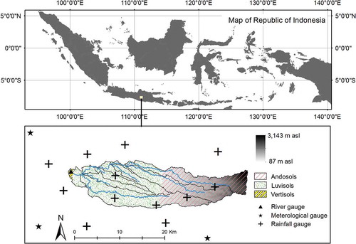
The Samin catchment experiences a tropical monsoon climate with distinct dry and wet seasons, where the former generally extends from May to October and the latter from November to April. Mean annual rainfall can be 1500 mm in dry years and reaches 3000 mm in wet years. The spatial rainfall pattern likely follows the orography, with a larger amount of rainfall in the upstream than in the downstream area. The mean daily temperature is approximately 26°C, with a mean daily minimum of 21.5°C and a mean daily maximum of 30.5°C. The mean annual potential evapotranspiration in the catchment ranges from 1400 to 1700 mm (Marhaento et al. 2017a). According to the Indonesia Statistical Bureau (BPS 2017), the population size at the sub-district level in the Samin catchment is about 800 000 inhabitants, with an average annual population growth over the period 1994–2010 of about 0.8%. In the same period, land use has changed significantly, with an increase in the settlement area and a decrease in the forest area (Marhaento et al. 2017a). Population growth in the Samin catchment has been projected to decrease over time, reaching 0.1% per year in 2035, as a result of a successful birth control programme as well as a transmigration programme (BPS 2013), which may affect future land-use change in the study catchment.

2.2 Data availability

To set up the hydrological model, spatial and non-spatial data were used. For the spatial data, land-use maps of 30-m spatial resolution for the years 1994, 2000, 2006 and 2013 were available for the study area from Marhaento et al. (2017a). A land-use spatial planning map of the study area for the period 2009–2029 was available from Central Java Provincial Government (2010). The topographic map contains information related to elevation, roads and locations of public facilities (e.g. hospitals, schools and offices) and is available from the Geospatial Information Agency of Indonesia at 1:25 000 scale. A soil map at a spatial resolution of 30 arcsec was taken from FAO, IIASA, ISRIC, ISSCAS, JRC (2012).

For the non-spatial data, daily water level data for the period 1990–2013 were available from the Bengawan Solo River Basin organization and converted into daily discharge data using the rating curves provided by the organization. Daily climate data for the period 1983–2013 were available from 11 rainfall stations and three climate stations within the surrounding catchments. Future climate data for the period 2030–2050 for different emission scenarios were obtained from SEACLID/CORDEX Southeast Asia (CORDEX-SEA), a consortium consisting of experts from 14 countries and 19 institutions that aims to downscale a number of global climate models (GCMs) from the Fifth Coupled Model Inter-comparison Project (CMIP5) for the Southeast Asian region. For Indonesia, the Indonesian Agency for Meteorology, Climatology and Geophysics (BMKG) provided the regional climate model (RCM) RegCM4 data at 25 km × 25 km resolution (Ngo-Duc et al. 2016), downscaled from the CSIRO Mk3.6.0 GCM. The rainfall and maximum and minimum temperature data are available on a daily basis for the period 1983–2005 to represent the baseline period, and for 2030–2050 to represent the future period. Two scenarios for the radiative forcing of future greenhouse gas emissions were applied, namely Representative Concentration Pathway (RCP) 4.5 and 8.5 to represent low emission and high emission scenarios, respectively. In addition to the RCM dataset, this study also used six additional GCMs from different sources in order to include the effect of climate model uncertainty. This study used GCMs rather than other RCMs to include climate model uncertainty because other RCMs are not available for the study catchment. Table 1 shows the characteristics of each GCM used in this study. These GCMs were selected after comparison of the mean annual rainfall in the study catchment from 26 GCMs listed in CMIP5, which showed significantly different changes in rainfall (even in the direction of change) between the baseline and future periods, resulting in a large uncertainty band in future climate variability. By taking GCMs with the most significant different directions and magnitudes, the results of the simulations using these selected GCM outputs will probably cover the full range of potential futures, including those that would follow from the outputs from other GCMs listed in CMIP5, including the ensemble mean. It should be noted that, for the mean annual rainfall used in the GCM selection, this study used the average value of RCP4.5 and RCP8.5 climate scenarios from the GCMs.

Table 1. List of CMIP5 GCMs used and their characteristics.

Model	Resolution (Lon. × Lat.)	Country of origin	Difference*	References
GFDL-ESM2M	2.5º × 2.0º	USA	− − −	Dunne et al. (2012)
CanESM2	2.81º × 2.79º	Canada	− −	Arora et al. (2011)
CSIRO-Mk3.6.0	1.875º × 1.86º	Australia	−	Collier et al. (2011)
MPI-ESM-LR	1.875º × 1.85º	Germany	+	Giorgetta et al. (2013)
MIROC5	1.41º × 1.39º	Japan	+ +	Watanabe et al. (2010)
NorESM1-M	2.5º × 1.875º	Norway	+ + +	Bentsen et al. (2013)

*Difference between baseline and future conditions, where “−” indicates that the mean annual rainfall in the future period is smaller and “+” that it is larger than in the baseline period.

3 Methods

3.1 Land-use change model

Future land-use distributions in the study catchment are based on two land-use scenarios, namely a business-as-usual (BAU) scenario and a controlled (CON) scenario. The BAU scenario represents a future situation where no measures are taken to control land-use change in the study catchment, whereas the CON scenario represents idealized land-use conditions that follow the spatial planning regulation.

3.1.1. Business-as-usual (BAU) scenario

Attempts were made to ensure that future land use in the study catchment under the BAU scenario is in accordance with the ongoing trends of land-use change. An integration of a Markov chain and a cellular automata model (CA–Markov) with multi-criteria evaluation (MCE) was used to project land-use changes in the catchment for the future period (i.e. 2030–2050). The CA–Markov model has been widely used to simulate land-use changes throughout the world (Myint and Wang 2006, Hyandye and Martz 2017). Compared to other models with a similar aim (e.g. GEOMOD, CLUE), the CA–Markov model has a high ability to simulate multiple land-use covers and complex patterns with smaller amounts of data and less computational effort (Eastman 2012). Along with the CA–Markov model, an MCE technique was used to support the decision processes of land allocations using different criteria of land-use suitability (Behera et al. 2012). The MCE uses factors and constraints for each land-use category. Different factors indicate the relative suitability of a specific land-use type that is generally based on a measured dataset (e.g. slope gradient, elevation and road distances), whereas constraints are used to exclude certain areas from consideration (e.g. protected area and water bodies).

Factors and constraints of each land-use type were selected based on the available spatial data (see Table 2). In order to make the factors and constraints spatially comparable, they were standardized using fuzzy membership functions with a range of 0–1, where a value closer to 1 indicates a stronger membership. Three types of fuzzy membership function were used, namely a monotonically increasing linear function (MIL), a monotonically decreasing linear function (MDL) and a monotonically increasing symmetric function (MIS). Subsequently, four fuzzy control points were determined, in which the first marks the location where the membership function begins to rise above 0, the second indicates where it reaches 1, the third indicates where the membership function drops below 1 again, and the fourth marks the point where it returns to 0. The four control points of the fuzzy membership function for each land-use class used in this study were adapted from Hyandye and Martz (2017). However, some changes were made for this study considering the local conditions (e.g. agricultural area was divided into paddy field and dryland farm) and data availability (e.g. population density was not included as a factor).

Table 2. Factors, membership functions, control points and constraints of the different land-use classes. MIL: monotonically increasing linear function; MDL: monotonically decreasing linear function; MIS: monotonically increasing symmetric function.

Land-use class	Factors	Membership functions	Control points	Constraints
Evergreen forest	Slope gradient	MIL	a = 25, b = maximum	Existing settlement
	Distance from road	MIL	a = 500, b = maximum	Existing paddy field
	Elevation (DEM)	MIL	a = 1500, b = maximum	Waterbodies
Mixed garden	Slope gradient	MIS	a = 8, b = 25, c = 25, d = 45	Protected area
	Distance from road	MDL	a = 100, b = maximum	Waterbodies
	Distance from existing settlement	MDL	a = 100, b = maximum	Existing settlement
Paddy field	Slope gradient	MIS	a = 0, b = 15, c = 25, d = 45	Protected area
	Distance from road	MDL	a = 0, b = maximum	Waterbodies
	Distance from existing settlement	MDL	a = 0, b = maximum	Existing settlement
Dryland farm	Slope gradient	MIS	a = 0, b = 15, c = 25, d = 45	Protected area
				Waterbodies
	Distance from road	MDL	a = 0, b = maximum	Existing settlement
Settlement	Distance from road	MDL	a = 0, b = maximum	Protected area
	Distance from existing settlement	MDL	a = 0, b = maximum	Waterbodies
	Slope gradient	MDL	a = 0, b = 45
	Distance from urban facilities	MDL	a = 0, b = maximum
Shrub land	Slope gradient	MIL	a = 15, d = maximum	Protected area
	Distance from road	MIL	a = 500, b = maximum	Waterbodies
	Distance from existing settlement	MIL	a = 500, b = maximum	Existing settlement
Waterbodies	Existing waterbodies	-	-	-

In this study, the Markovian transition area matrix was generated using two recent land-use maps for the years 2006 and 2013. However, we applied a boundary condition for the settlement area by determining the settlement area in 2050 based on a linear relationship between the changes in settlement area estimated from historical land-use maps (Marhaento et al. 2017a) and population size in the same years (see Fig. 2(a)). Population in 2050 was obtained using a second-order polynomial function that can represent a decrease in the population growth in the future, based on the information from the Indonesia Statistical Bureau (BPS 2013) (Fig. 2(b)). The results suggest that the settlement area in the study catchment in 2050 will be 50.2% of the study area. We applied this boundary condition in the simulation through a modification of the time lags of the model simulation until the model closely projected a settlement area in 2050 of about 50% of the study area. The projected annual land-use distributions from 2030 to 2050 resulting from the fitted model were used as land-use inputs in the SWAT simulations under the BAU scenario. For this study, spatial data preparation and land-use simulations were executed using IDRISI Selva v.17 software (Eastman 2012).

Figure 2. (a) Linear relationship between the settlement area (in %) and population size and (b) second-order polynomial function of the population growth in the Samin catchment.

3.1.2 Controlled scenario

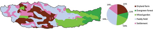
In the controlled (CON) scenario, future land use in the study catchment was assumed to follow the spatial planning map. A pre-processing analysis was carried out in order to convert a printed map of the spatial planning map into a digital map. Furthermore, we changed the classification of the spatial planning map to be comparable with the land-use classification from Marhaento et al. (2017a). Figure 3 shows the spatial planning map of the study catchment with reclassified land-use types. According to the spatial planning map, in the year 2029, agricultural area (i.e. paddy field and dryland farm) will be the dominant land-use type in the study catchment, covering 55% of the study area, followed by forest area (i.e. evergreen forest and mixed garden, 31%) and settlements (14%). Forest area is dominant in the upstream area, whereas agricultural area and settlements are dominant in the downstream area. We used the projected land-use distribution in 2029 from the spatial planning map and the land-use map for the year 2013 as inputs in the CA–Markov model in order to simulate annual land-use distribution in the future period (i.e. 2030–2050). The output of the model was used as land-use input in the SWAT simulations under the CON scenario.

Figure 3. Projected land-use map of the Samin catchment for 2029 according to the spatial planning map of the Central Java Provincial Government.

3.2 Climate change model

Generally, GCM and RCM outputs are biased, which hampers the direct use of GCM or RCM data to assess the impact of climate change on hydrological processes (Teutschbein and Seibert 2012). Thus, there is a need to correct these outputs before they can be used for regional impact studies. In this study, we used different bias correction methods to correct RCM and GCM output. However, considering that the size of the study catchment is not comparable with the spatial resolution of the applied RCM and GCM outputs, we used the average values of rainfall and temperature from six RCM and three GCM grid cells located near the study catchment. We did this in order to minimize the bias due to inhomogeneity of a single station because of systematic bias in the model (Murphy et al. 2004, Gubler et al. 2017).

For the RCM data, the distribution mapping method and the variance scaling method were used to correct biases in rainfall and maximum and minimum temperatures, respectively. We selected these methods having performed an accuracy assessment based on a split sample test (Klemeš 1986), where the period 1983–1997 was the calibration period and 1998–2005 was the validation period, for different bias correction methods (i.e. linear scaling, power transformation, distribution mapping). We found that these methods outperformed other methods based on their coefficient of determination (R²) against the observed rainfall and maximum and minimum temperatures. For rainfall, the distribution mapping method resulted in R² of 0.77 with a root mean square error (RMSE) of about 88 mm/month, whereas the linear scaling and power transformation methods resulted in R² of 0.53 (RMSE = 108 mm/month) and 0.56 (RMSE = 107 mm/month), respectively. For the maximum and minimum temperatures, the variance scaling method resulted in R² of 0.62 (RMSE = 1.1°C), whereas the linear scaling and distribution methods resulted in R² of 0.51 (RMSE = 1.3°C), and 0.48 (RMSE = 1.4°C), respectively. However, it should be noted that all bias correction methods improved the raw RCM-simulated rainfall and maximum and minimum temperatures. For the six additional GCMs, we applied a delta change method to correct biases of the GCM-simulated rainfall and maximum and minimum temperatures. Rather than using the GCM simulations of future conditions directly, the delta change method uses the differences between GCM-simulated historic and future conditions for a perturbation of observed data. For a detailed description of each method, we refer to Teutschbein and Seibert (2012) and Fang et al. (2015).

3.3 Hydrological model

The Soil and Water Assessment Tool (SWAT) model (Arnold et al. 1998) was used to simulate hydrological processes in the study catchment. The SWAT model is a physically based semi-distributed model that divides a catchment into sub-catchments and then further into hydrological response units (HRUs) for which a land-phase water balance is calculated (Neitsch et al. 2011). Runoff from each HRU (i.e. combinations of land use, soil and slope) is aggregated at sub-catchment level and then routed to the main channel for which the catchment water balance is calculated. In a previous study, we showed the suitability of SWAT to attribute changes in the water balance to land-use change in the Samin catchment (Marhaento et al. 2017a). The SWAT model set-up in this study used the same settings as in Marhaento et al. (2017a). Therefore, we only present a brief summary of the model set-up and calibration results here.

Eleven sub-catchments, ranging in size from 0.12 to 83 km² were delineated based on the digital elevation model (DEM). In addition, the DEM was used to generate a slope map based on the slope classification from the Guidelines of Land Rehabilitation from the Ministry of Forestry (1987). Land-use codes from the SWAT database, namely AGRR, FRSE, FRST, RICE, URMD, LBLS and WATR, were assigned to denote dryland farming, evergreen forest, mixed garden, paddy field, settlements, shrub land and water, respectively. For the settlement land use, we used the assumption that the settlement area is not fully impervious and in between the houses has some pervious spaces that are often used as domestic yards. Thus, we used the class Urban Residential Medium Density (URMD) in the SWAT model to assign parameters to the settlement area. The URMD assumes an average of 38% impervious area in the settlement area (Neitsch et al. 2011), which is similar to the settlement conditions in the study catchment.

The HRUs of the study catchment were created by spatially overlaying a land-use map with seven classes (i.e. AGRR, FRSE, FRST, RICE, URMD, LBLS and WATR), a slope map with five classes (i.e. 0–8%, 8–15%, 15–25%, 25–45% and > 45%), and a soil map with three classes (i.e. luvisols, andosols and vertisols) resulting in about 359 HRUs. The Hargreaves method was used to calculate reference evapotranspiration because it requires only temperature data that are available for the past and future periods in this study. The Soil Conservation Service Curve Number (SCS CN) and the Muskingum method were used to calculate surface runoff and flow routing, respectively.

Following the procedure of Abbaspour et al. (2015), six SWAT parameters, namely CN2, SOL_AWC, ESCO, CANMX, GW_DELAY and GW_REVAP, were identified as the most sensitive parameters, and these were calibrated using the Latin Hypercube Sampling approach from the Sequential Uncertainty Fitting version 2 (SUFI-2) in the SWAT-Calibration and Uncertainty Procedure (SWAT-CUP) package. The calibration period was 1990–1995, assuming that this period is a reference period when land-use change and climate change had small impacts on hydrological processes (Marhaento et al. 2017a). First, parameter ranges were determined based on minimum and maximum values allowed in SWAT. A number of iterations were performed where each iteration consisted of 1000 simulations with narrowed parameter ranges in subsequent calibration rounds. Simulations for model calibration were assessed on a monthly basis and the Nash Sutcliffe Efficiency (NSE) criterion was used as the objective function, similarly to in, for instance, Setegn et al. (2011) and Zhang et al. (2015). Besides the NSE, other model performance statistics, including percent bias (PBIAS), R², RMSE and the mean absolute error (MAE), were calculated to evaluate the performance of the hydrological models. The results of the model calibration show that the simulated mean monthly discharge in the calibration period agrees well with the observed records, with NSE, PBIAS, R², RMSE and MAE values of 0.78, −7.8, 0.78, 3.6 m³/s and 2.7 m³/s, respectively. For the validation period (1996–2013), the NSE model performance of the calibrated SWAT model is 0.70 and values for the other metrics (PBIAS, R², RMSE and MAE), were 0.6, 0.76, 3.4 m³/s and 2.5 m³/s, respectively.

3.4 Future hydrological responses to land-use and climate change scenarios

Future hydrological processes in the study catchment were simulated using the calibrated SWAT model, using inputs from the bias-corrected RCM and GCMs for the period 2030–2050 and the projected land-use distributions. For the baseline conditions, we used the output of the SWAT simulations forced by the bias-corrected RCM data and the observed data, where both datasets cover the period 1983–2005. The baseline condition simulated with the bias-corrected RCM data was used as a baseline condition for the future simulation forced by the RCM dataset, whereas the baseline condition simulated by the observed data was used as a baseline condition for the future simulation forced by the GCM dataset. In addition, two land-use distributions for the years 1994 and 2000 were used in the simulation to represent land-use conditions in the baseline period. We used the Land Use Update (LUP) tool in ArcSWAT (Marhaento et al. 2017a) to incorporate land-use change in the SWAT simulations, in which land use was initially assumed as that reported for 1994, and updated by the land use for 2000 when the simulation date entered 1 January 2000. The LUP tool was also used to incorporate land-use change in the simulations for the future period (i.e. 2030–2050), where in the simulations we annually updated the land-use information from the land-use change model. Table 3 shows the scenario simulations executed in this study including assessment of the effects of land-use change only (LUC), climate change only (CC) and combined land-use and climate change (LUC+ CC) scenarios on hydrological processes. For each scenario, several hydrological components, namely precipitation (P), potential evapotranspiration (PET), streamflow (Q), actual evapotranspiration (ET), surface runoff (Q_s), lateral flow (Q_l) and baseflow (Q_b) were calculated and compared to the baseline conditions. It should be noted that this study is carried out at the catchment level since the model was calibrated and validated based only on a single discharge station located at the catchment outlet. We did not assess the impacts of land-use and climate changes on the water balance at a finer scale than the catchment scale (i.e. sub-catchment) because impact assessment at the sub-catchment scale, for which the calibration has not been carried out, may not be justified (e.g. Ewen et al. 2006). In addition, this study used the average value of six RCM and three GCM grid cells to represent future climate conditions of the study catchment. Consequently, relatively small water balance variations from different climate conditions in different sub-catchments were found.

Table 3. Future land-use and climate change scenarios as inputs for the SWAT model. NLUC: no land-use change; NCC: no climate change; BAU: business-as-usual scenario; CON: controlled scenario; RCP4.5 and RCP8.5: climate change scenarios under Representative Concentration Pathways 4.5 and 8.5, respectively. For simulations under CC and LUC + CC scenarios, we used outputs from one RCM and six GCMs as model inputs to include climate model uncertainty.

Scenarios		Land-use change
		NLUC	BAU	CON
Climate change	NCC	Baseline	BAUNC^a	CONNC^a
	RCP4.5	NC4.5^b	BAU4.5^c	CON4.5^c
	RCP8.5	NC8.5^b	BAU8.5^c	CON8.5^c

^aLUC scenarios.

^bCC scenarios.

^cLUC + CC scenarios.

4 Results

4.1 Land-use change

As shown in Table 4, land use in the study catchment in 2050 under the BAU scenario is predominantly settlements, followed by paddy field, dryland farm, mixed garden, evergreen forest, shrub land and waterbodies. Settlement refers to a built-up area and its surroundings; paddy field is agricultural land that consists of rice paddy fields with an intensive irrigation system; dryland farm is an agricultural area for seasonal crop production; mixed garden is community forest that consists of multipurpose trees (e.g. fruits, fuel wood, etc.), often combined with seasonal crops on the same unit of land; evergreen forest is a homogeneous forest area that consists mainly of Pinus merkusii tree species; shrub land is an abandoned area covered by herbaceous plants; and waterbodies refers to rivers and ponds.

Table 4. Land-use distribution (in %) in the years 2000 and 2050 for different scenarios.

Land-use class		Reference (2000)	Future (2050)
			BAU		CON
		LU 2000	LU 2050	∆	LU 2050	∆
1. Forest area		42.2	7.2	−35	30.3	−11.9
	a. Evergreen forest	3	2.3	−0.7	13.2	10.2
	b. Mixed garden	39.2	4.9	−34.3	17.1	−22.1
2. Agricultural area		36.9	40.4	3.5	52.1	15.2
	a. Paddy field	28.2	22.2	−6	34	5.8
	b. Dryland farm	8.7	18.2	9.5	18.1	9.4
3. Settlement		16.3	50.2	33.9	17.3	1
4. Shrub land		4.3	1.9	−2.4	0	−4.3
5. Waterbodies		0.3	0.3	0	0.3	0

In comparison to the year 2000, forest area (i.e. evergreen forest and mixed garden) and shrub land decreased by 35% and 2.4%, respectively, while agricultural area (i.e. paddy field and dryland farm) and settlements increased by 3.5% and 33.9%, respectively (Table 4). The settlement area significantly increased in the down- and mid-stream areas, where mixed garden and paddy field were converted to impervious areas. In the upstream area, the dryland farm land use was mainly converted to mixed garden and shrub land, as shown in Figure 4.

Figure 4. Land-use cover of the Samin catchment in (a) 2000, (b, d) 2030 and 2050 under business-as-usual (BAU) scenario, and (c, e) 2030 and 2050 under controlled (CON) scenario.

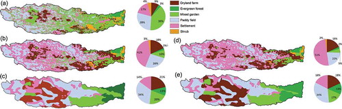
Under the CON scenario, land use in 2050 is predominantly paddy field, followed by dryland farm, settlements, mixed garden, evergreen forest and waterbodies. In comparison to the year 2000, mixed garden and shrub land decreased by 22.1 and 4.3%, respectively, while agricultural area, evergreen forest and settlements increased by 15.2%, 10.2% and 1%, respectively. Figure 4 shows that, under the CON scenario, forests are located in the upstream area, while agricultural area and settlements are in the down- and mid-stream areas. It should be noted that, in this scenario, the evergreen forest area will increase, while the mixed garden area will decrease, resulting in a net decrease in forest area of 11.9%.

4.2 Climate change

Figure 5 shows the changes in mean annual rainfall from the RCM and GCMs under RCP4.5 and RCP8.5 in the future period (2030–2050) relative to the baseline period (1983–2005). Based on the RCM, the mean annual rainfall in the study catchment is projected to decrease by 412 mm (−20%) under RCP4.5 and 505 mm (−25%) under RCP8.5. The direction of change in the mean annual rainfall for the RCM is similar to those for three of the GCMs (i.e. GFDL-ESM2M, CanESM2 and CSIRO-Mk3.6.0), which projected a decrease in mean annual rainfall ranging from 8 mm (−0.4%) to 193 mm (−18%) under RCP4.5 and from 22 mm (−1%) to 343 mm (−17%) under RCP8.5. In contrast, the other three GCMs (MIROC5, MPI-ESM-LR and NorESM1-M) showed the opposite direction of change in the mean annual rainfall over the study area. These GCMs project an increase in mean annual rainfall in the future ranging from 91 mm (+5%) to 384 mm (+19%) under RCP4.5 and from 87 mm (+4%) to 287 mm (+15%) under RCP8.5. Although the RCM-simulated rainfall was downscaled from the CSIRO Mk.3.6.0 GCM, the magnitude of change of the two is different, in particular under the RCP4.5 scenario. This is probably due to systematic biases in the RCM, which makes it independent from its driving datasets because of its physics parameterization (Murphy et al. 2004) and application of the bias-correction method (Themeßl et al. 2012).

Figure 5. Changes in mean annual and monthly rainfall in the Samin catchment in the future period (2030–2050) relative to the baseline period (1983–2005) under RCP4.5 and RCP8.5 scenarios.

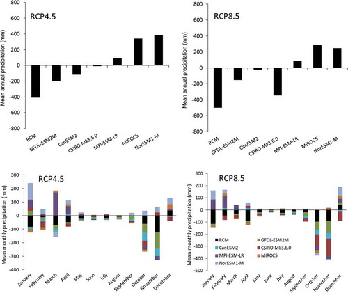
While different climate models show inconsistent directions of change for future rainfall, all climate models project a similar direction of change for the maximum and minimum temperatures, although with slightly different magnitudes. For the RCM, the mean annual maximum and minimum temperatures increase for both scenarios, by +1.0°C and +1.3°C, respectively, under RCP4.5, and by +0.7°C and +1.4°C, respectively, under RCP8.5. All GCMs projected an increase of about +1°C in the mean annual maximum and minimum temperatures in the future period compared to the baseline period under both RCP4.5 and RCP8.5 scenarios.

4.3 Future hydrological response

4.3.1 Effects of land-use change

In comparison to the baseline conditions (1983–2005), simulations under land-use change scenarios indicated a decrease in the mean annual ET and an increase in the mean annual Q and Q_s (Fig. 6). However, the directions of change were different for Q_l and Q_b. Under BAU, Q_l increases and Q_b decreases, while under CON, Q_l decreases and Q_b increases. We find that under BAU the mean annual ET decreases by 15%, which is larger than the decrease of 7.4% under CON. A decrease in the mean annual ET under both scenarios is compensated by an increase in the mean annual Q with the same magnitude. More pronounced changes occur in the fraction of Q that becomes Q_s, Q_l and Q_b. Under BAU, the mean annual Q_s and Q_l increase by 40% and 20%, respectively, at the expense of Q_b, which decreases by 3%. Under CON, the mean annual Q_s increases by 16% and the mean annual Q_b by 6%, while the mean annual Q_l was relatively constant. At a monthly scale (Fig. 6(b)), the simulated Q under both land-use change scenarios is higher than in the baseline period during the wet season and similar to the baseline period during the dry season. The mean monthly Q under the BAU and CON scenarios reaches its peak in February, with a value of 175 mm (+41%) and 149 mm (+20%), respectively.

Figure 6. (a) Change in the mean annual water balance components under different land-use change scenarios compared to the baseline period. (b) Mean monthly streamflow under different land-use change scenarios.

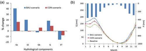
Changes in the hydrological responses as a result of land-use changes were mainly affected by changes in the Curve Number (CN) parameter in the simulation. Table 5 shows the relationship between changes in the weighted CN value and mean annual Q and ET under different land-use change scenarios. The results show that an increase in the weighted CN value at catchment level for both scenarios resulted in an increase in the mean annual Q and a decrease in the mean annual ET, where the increase in the weighted CN value under the BAU scenario is larger than that under the CON scenario.

Table 5. Weighted curve number (CN) value, mean annual streamflow (Q) and evapotranspiration (ET) for different land-use types under different land-use change scenarios. BAU: business-as-usual; CON: controlled.

Variables	LUC scenario	Evergreen forest	Mixed garden	Paddy field	Dryland farm	Settlement	Shrub	Water	Catchment averaged
Weighted CN	Baseline	47.3	59.8	70.0	71.6	77.4	50.3	78.2	63.42
	BAU	46.8	54.5	68.6	69.4	76.3	50.2	78.2	69.71
	CON	46.8	52.6	67.9	75.2	77.3	50.2	78.2	66.23
Q (mm)	Baseline	726	714	1060	1046	1194	1036	0	906
	BAU	730	722	1045	1031	1193	1055	0	1068
	CON	730	716	1037	1078	1197	1071	0	984
ET (mm)	Baseline	1331	1332	985	1002	860	1015	1179	1144
	BAU	1328	1333	1001	1021	862	1002	1179	984
	CON	1328	1336	1008	970	859	981	1179	1066

4.3.2 Effects of climate change

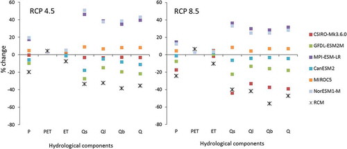
There is a large uncertainty in the future mean annual P for both RCP4.5 and RCP8.5, which causes a large variation in the projected water balance components (Fig. 7). Projected changes in the mean annual P under different RCP scenarios range from −20% to +19% under RCP4.5 and from 25% to +15% under RCP8.5. Together with an increase in the simulated PET of about 3%, changes in the mean annual P from both RCP scenarios cause a significant change in the mean annual Q as well as in the fractions of flow that become Q_s, Q_l and Q_b, while changes in ET are relatively minor. Under RCP4.5, projections of the mean annual Q and ET range from −35% to +43% and from −7% to +5%, respectively. Pronounced changes can be observed for the mean annual Q_s (ranging from −33% to +50%), Q_l (−32% to +38%) and Q_b (−38% to +39%). Under RCP8.5, projections of the mean annual Q and ET range from −47% to +32% and −10% to +5%, respectively, whereas changes in the mean annual Q_s, Q_l and Q_b range from −44% to +36%, −41% to +29%, and −56% to +28%, respectively. The large ranges in the projections for the mean annual water balance components likely result from the differences in the projected P from the different climate models. It should be noted that the RCM downscaled from a CSIRO Mk.3.6.0 GCM projected a (very) significant decrease in the mean annual P for both scenarios, resulting in pronounced changes in the mean annual Q, Q_s, Q_l and Q_b.

Figure 7. Changes in the water balance components (in %) compared to the baseline period under RCP4.5 and RCP8.5 scenarios for different climate models.

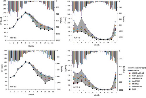
At a monthly scale, most climate models under RCP4.5 and RCP8.5 project a decrease in ET during the dry season and an increase during the wet season (Fig. 8). A large uncertainty is found for the dry season, for which some climate models under RCP8.5 project a significant decrease in the mean monthly ET, in particular for the simulation using the RCM data. For Q, a large uncertainty is found during the wet season, because different climate models project different directions of change, in particular under RCP4.5. Under RCP8.5, the direction of change is evident, with most climate models projecting a decrease of Q from April to December.

Figure 8. Mean monthly ET and Q from different climate models under RCP4.5 and RCP8.5 scenarios.

4.3.3 Combined effects of land-use change and climate change

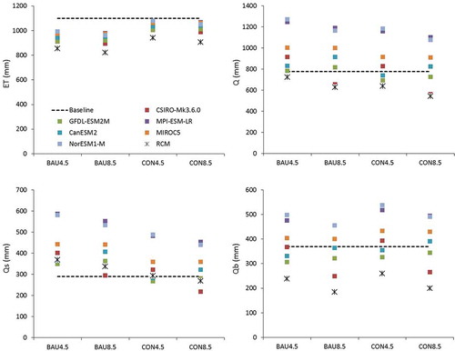
When land-use and climate change scenarios are combined, the effects on the water balance components are pronounced, as shown in Figure 9. It should be noted that in Figure 9 we used a single line to represent the baseline conditions to simplify the figure. This line is the average value of the baselines from the RCM and GCMs. The results show that the mean annual ET decreases, with the greatest decrease under the BAU8.5 scenario (ranging from −10% to −25%) and the smallest under the CON4.5 scenario (−1% to −14%). The direction of change in the mean annual ET under combined climate and land-use change scenarios is similar to the ET changes found when we considered land-use change only. The mean annual Q is mostly projected to increase under the BAU4.5 scenario (from −7% to +64%), where only the simulation with RCM data projected a decrease in Q. Under the BAU8.5 and CON4.5 scenarios, the projected changes in the mean annual Q range from −18% to +53% and −19% to +52%, respectively. The largest uncertainty in change in the mean annual Q is found under the CON8.5 scenario, in which it will change by −30% to +42%. An increase in the mean annual Q is observed under the BAU4.5 scenario, although some climate models predict a decrease in the mean annual rainfall. Changes in the mean annual Q due to land-use change are amplified under wetting climate scenarios (projection of an increase in the future rainfall from the climate models), where the mean annual Q increases by about 64% under scenario BAU4.5, which is about 40% more than under the land-use change only scenario. Similarly, there is a significant increase in the mean annual Q_s in particular under the BAU4.5 and BAU8.5 scenarios, although the RCM and some GCMs project a decrease in the mean annual rainfall. The mean annual Q_s is projected to increase by +21% to +102% and by +2% to +91% under the BAU4.5 and BAU8.5 scenarios, respectively. Changes in the mean annual Q_s are pronounced for wetting climate scenarios, where the mean annual Q_s is projected to increase by about 100% compared to the baseline conditions, which is 60% more than under the land-use change only scenario. For Q_b, it is observed that scenarios show increases as well as decreases in the mean annual Q_b, resulting in a large uncertainty. The directions of change in the mean annual Q_b under different scenarios are similar to those under the climate change only scenario. The CON4.5 scenario projected the largest change in mean annual Q_b, with a range from −30% to +46%, subsequently followed by the CON8.5, BAU4.5 and BAU8.5 scenarios.

Figure 9. Predicted mean annual water balance components for different combinations of climate change and land-use change scenarios.

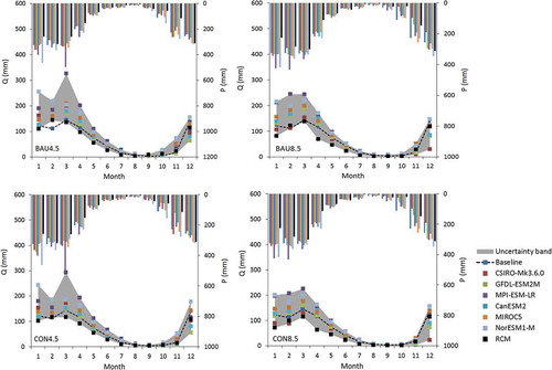
At a monthly scale, most of the scenarios project an increase in the mean monthly Q from January to March, where changes in the mean monthly Q range from +60% to +120% compared to the baseline period (Fig. 10). During the dry season, a large uncertainty is found for all scenarios, which projected decreases as well as increases in the mean monthly Q. At the start of the wet season (i.e. November), most scenarios projected a decrease in the mean monthly Q, where the largest decrease is found under the CON85 scenario (ranging from −84% to +14%), followed by BAU85, CON45 and BAU45.

Figure 10. Mean monthly streamflow for different combinations of land-use change and climate change scenarios.

5 Discussion

In the Samin catchment, changes in land use are mainly controlled by internal factors, such as expansion of agriculture and settlements, whereas changes in climate variability are considered as externally driven. Both play a significant role in changing hydrological processes of the catchment. Using a modelling approach, this study assesses individual and combined effects of future land-use and climate change on the water balance components in the Samin catchment.

5.1 Effects of future land-use change

Findings show that when future land-use changes under a business-as-usual (BAU) scenario, mean annual evapotranspiration will decrease, resulting in an increase in the mean annual streamflow. The mean annual surface runoff and lateral flow are projected to increase almost twofold, but baseflow will decrease. A massive land-use conversion from vegetated area into settlement area as suggested by the BAU scenario will significantly reduce canopy interception and soil infiltration capacity, resulting a large fraction of rainfall being transformed into surface runoff (Bruijnzeel 2004, Valentin et al. 2008, Marhaento et al. 2017a). As a result, under BAU, the Samin catchment will face an increasing risk of disastrous events such as flash floods, landslides and severe soil erosion. Those risks can potentially be reduced by introducing and enforcing a land-use planning regulation. We find that the allocation of forest area to the upstream part of the catchment and agriculture to the midstream part, while maintaining the settlement area, as suggested by the CON scenario, would significantly reduce the mean annual surface runoff and lateral flow, while the mean annual baseflow would increase. A large fraction of vegetated area (i.e. evergreen forest) may lead to an increase in the water storage capacity of the soil due to greater root penetration and biotic activity in the upper soil layers, resulting in a larger infiltration rate and ground water recharge (Bruijnzeel 1989, 2004, Guevara-Escobar et al. 2007). With more water infiltrated and stored into the soil, a more balanced water distribution between wet and dry seasons can be expected. The directions of change in the water balance components by land-use change in this study are in line with other studies in the tropics from Bruijnzeel (1989), Valentin et al. (2008), Remondi et al. (2016) and Marhaento et al. (2017a).

5.2 Effects of future climate change

When considering only climate change, findings show that changes in the mean annual rainfall may have large impacts on the water availability of the Samin catchment. An increase (or decrease) in the mean annual rainfall may result in a large increase (or decrease) in the streamflow and in the fractions of flow that become surface runoff, lateral flow and baseflow, while changes in ET are relatively minor. However, small increases in rainfall are likely to have little impact on the water balance. More significant impacts on the water balance can be observed if the changes in the mean annual rainfall are larger than 10%, where the impacts on streamflow and on the fractions of flow that become surface runoff, lateral flow and baseflow can be double the changes in rainfall. Accordingly, changes in the fraction of flow becoming surface runoff, lateral flow and baseflow can be larger under climate change scenarios than land-use change scenarios. These findings are similar to the results of Mango et al. (2011) and Liu et al. (2011). The rising temperature causes an increase in the potential evapotranspiration, which may affect the mean annual ET due to an increase in the available energy (Budyko 1974). However, this study finds that changes in annual ET are likely attributed to changes in annual rainfall, where the variations of ET follow the variations of rainfall. Thus, an increase in ET is found during the wet season while a significant decrease in ET is found during the dry season. These findings are in line with Budyko (1974), who argues that changes in evapotranspiration are determined by the balance between precipitation and evaporative demands.

5.3 Combined effects of future land-use change and climate change

The findings show that both land-use change and climate change contribute to changes in the water balance components, but each driver has a specific contribution to the water balance alteration. Under combinations of land-use and climate change scenarios, changes in the annual evapotranspiration are likely attributed to land-use change, while changes in the annual baseflow are likely attributed to climate change. It should be noted that this study used two completely different land-use scenarios, where the BAU scenario represents deforestation and the CON scenario (partly) reforestation. Thus, changes in annual evapotranspiration under different land-use change scenarios can be clearly observed, since trees are generally known to have higher evapotranspiration rates than other land uses (Bruijnzeel 1989, 2004, Marhaento et al. 2017a). The presence of forests can increase the annual evapotranspiration from both canopy interception and plant transpiration, so that under the BAU scenario there will be a significant decrease in the annual evapotranspiration. However, one cannot neglect the role of climate variability to control changes in the annual evapotranspiration, since evapotranspiration is largely influenced by precipitation (Budyko 1974, Liu et al. 2011). At the monthly scale, evapotranspiration is close to its potential value during the wet season, since rainfall supplies sufficient water, whereas in the dry season, the evapotranspiration capacity is mainly determined by the antecedent soil moisture and influenced by different land-cover types (Liu et al. 2011).

The magnitude of changes in annual baseflow is mainly determined by climate change (i.e. changes in rainfall), where the directions of change in annual Q_b under different scenarios are similar to those under the climate change only scenario. We found a small effect of land-use change on the changes in the annual baseflow, with a larger baseflow under the CON scenario. However, the magnitude of changes in baseflow under different land-use scenarios was smaller than expected. According to Ilstedt et al. (2007), the presence of forests can result in more baseflow due to an enhanced groundwater recharge. Apparently, in this catchment, the effects of land-use change on the baseflow are offset by climate change. Thus, more research is needed to assess the attribution of changes in the baseflow to land-use change and climate change.

Combined land-use change and climate change have a more pronounced effect on the streamflow and surface runoff. A projected increase in rainfall accompanied by the deforestation scenario (BAU scenario) will have more significant impacts on streamflow and surface runoff than land-use change or climate change acting alone (Legesse et al. 2003, Hejazi and Moglen 2008, Khoi and Suetsugi 2014). Moreover, at the monthly scale, the streamflow originating from surface runoff significantly increases during the wet season and decreases during the dry season, indicating that more extreme events (i.e. droughts and floods) will potentially occur in the future. Under the land-use planning scenario (CON scenario), the effects can be reduced, but only by less than 20%. Thus, more measures (e.g. soil conservation) are required in addition to land-use planning in order to enhance infiltration and aquifer recharge and subsequently reduce risks due to land-use and climate change impacts.

Besides resulting in more pronounced effects on the water balance alteration, combined climate change and land-use change also resulted in a “neutralizing” effect, where the combined effects resulted in less significant impacts because the effects of land-use and climate changes on hydrological processes were acting in opposite directions. In this study, this neutralizing effect occurred in particular during the dry season, in which the hydrological variations are mainly driven by climate variability rather than by land-use change. During dry conditions, changes in the hydrological processes were small despite the fact that land use has changed significantly, as can be seen under the BAU scenario. For this reason, we agree with Zhang et al. (2016), who argued that the role of land-use change should not be overlooked under dry climatic conditions.

5.4 Limitations and uncertainties

This study couples a land-use change model, a climate change model and a hydrological model, whereby each model can be a source of uncertainty affecting the results. For the land-use change model, we used an integration of the CA–Markov and MCE techniques to project future land-use distributions. However, this method bases land use in the future on extrapolation of trends, while future trends are obviously uncertain due to uncertainties in e.g. future population growth. Therefore, we used a boundary condition in the simulations to constrain the future land-use distributions. For the climate change model, large model uncertainties occur due to model choices, where different climate models result in different directions of change in the projected rainfall. Therefore, this study employed six additional GCMs that were selected based on different directions of change in future rainfall to include climate model uncertainty. However, uncertainties from the climate models can be larger due to other sources of uncertainty, for instance from the model structure (e.g. choice of spatial resolution, the set of processes included in the model, basic assumptions on parameterization) and application of statistical downscaling methods (Murphy et al. 2004). For the selection of GCMs, the use of bias-corrected GCMs provided by ISIMIP (www.isimip.org) can be considered for further research, since this consortium has incorporated more specific information for different sectors (e.g. the agriculture sector) in their climate model scenarios. In addition, for further research it is suggested to downscale the climate model outputs based on the climatological gauge network in order to provide a better assessment of climate change impacts on hydrological processes at the catchment scale. For the hydrological model, sources of uncertainty can be present due to the model structure (e.g. model assumptions, equations) as well as data inputs (e.g. lack of relevant spatial and temporal variability of data on rainfall, soils, land uses and topography). It should be noted that in this study the SWAT model was mainly calibrated and validated for streamflow and not specifically for other water balance components such as ET, Q_b, Q_i and Q_b. Thus, the results of the analysis regarding these water balance components should be interpreted taking into account the uncertainty. In addition, this study used a coarse soil map, which may result in too much generalization of the nature of the soils in the study catchment. Moreover, the scenario settings used in this study follow a single-factor fixed method, which does not take into account atmospheric feedbacks of land surface processes (Blöschl et al. 2007). Considering these uncertainties, accumulation of errors may affect the results.

6 Conclusions

We have assessed the separate and combined impacts of projected future changes in land use and climate on the water balance components in the Samin catchment. The results show that, individually, land-use and climate change can result in changes in the water balance components, but that more pronounced changes will occur if the drivers are combined, in particular for the mean annual streamflow and surface runoff. When combining the RCP4.5 climate scenario and business-as-usual (BAU) land-use scenario, the mean annual streamflow and surface runoff are expected to change by −7% to +64% and +21% to +102%, respectively, which is 40% and 60% more than when land-use change is acting alone. When the BAU scenario is replaced by the controlled (CON) land-use scenario, the mean annual streamflow and surface runoff reduce by up to 10% and 30%, respectively, while the mean annual baseflow and evapotranspiration increase by about 8% and 10%, respectively. The findings show that land-use planning can be one of the promising measures to reduce future water-related risks in the Samin catchment. However, it remains a challenge to accurately predict the future hydrological changes due to land-use and climate change, since there are various uncertainties, in particular associated with future climate change scenarios.

Acknowledgements

The authors acknowledge the Bengawan Solo River Basin Organization (BBWS Bengawan Solo), the Bengawan Solo Watershed Management Agency (BP DAS Bengawan Solo) and the Indonesian Meteorological, Climatological, and Geophysical Agency (BMKG) for providing the hydrological and climatological data. We thank Dr Ardhasena Sopaheluwakan and his team of the Climate and Air Quality Research group of BMKG for valuable discussions about the CORDEX-SEA dataset.

Disclosure statement

No potential conflict of interest was reported by the authors.

Additional information

Funding

The first author expresses his appreciation to the Directorate General of Higher Education, Ministry of Research, Technology and Higher Education of the Republic of Indonesia, for the financial support during his PhD project [BPPLN DIKTI 2013].

References

- Abbaspour, K.C., et al., 2015. A continental-scale hydrology and water quality model for Europe: Calibration and uncertainty of a high-resolution large-scale SWAT model. Journal of Hydrology, 524, 733–752. doi:10.1016/j.jhydrol.2015.03.027
- Aldrian, E. and Djamil, Y.S., 2008. Spatio-temporal climatic change of rainfall in East Java Indonesia. International Journal of Climatology, 28 (4), 435–448. doi:10.1002/(ISSN)1097-0088
- Amien, I., et al., 1996. Effects of interannual climate variability and climate change on rice yield in Java, Indonesia. Water, Air, and Soil Pollution, 92 (1–2), 29–39.
- Arnold, J.G., et al., 1998. Large area hydrologic modeling and assessment part I: model development. Journal of the American Water Resources Association, 34 (1), 73–89. doi:10.1111/jawr.1998.34.issue-1
- Arora, V.K., et al., 2011. Carbon emission limits required to satisfy future representative concentration pathways of greenhouse gases. Geophysical Research Letters, 38, 5. doi:10.1029/2010GL046270
- Beck, H.E., et al., 2013. The impact of forest regeneration on streamflow in 12 mesoscale humid tropical catchments. Hydrology and Earth System Sciences, 17 (7), 2613–2635. doi:10.5194/hess-17-2613-2013
- Behera, D., et al., 2012. Modelling and analyzing the watershed dynamics using Cellular Automata (CA)–markov model–A geo-information based approach. Journal of Earth System Science, 121 (4), 1011–1024. doi:10.1007/s12040-012-0207-5
- Bentsen, M., et al., 2013. The Norwegian earth system model, NorESM1-M—part 1: description and basic evaluation of the physical climate. Geoscientific Model Development, 6 (3), 687–720. doi:10.5194/gmd-6-687-2013
- Blöschl, G., et al., 2007. At what scales do climate variability and land cover change impact on flooding and low flows? Hydrological Processes, 21 (9), 1241–1247. doi:10.1002/(ISSN)1099-1085
- BPS, 2013. Karanganyar and sukoharjo in figures 2013. Statistical Bureau of Karanganyar and Sukoharjo Regency. Indonesia: Ministry of Home Affairs.
- BPS, 2017. Karanganyar and sukoharjo in figures 2017. Statistical Bureau of Karanganyar and Sukoharjo Regency. Indonesia: Ministry of Home Affairs.
- Bruijnzeel, L.A., 1989. (De)forestation and dry-season flow in the tropics: A closer look. Journal of Tropical Forest Science, 1 (3), 229–243.
- Bruijnzeel, L.A., 2004. Hydrological functions of tropical forests: not seeing the soil for the trees? Agriculture, Ecosystems & Environment, 104 (1), 185–228. doi:10.1016/j.agee.2004.01.015
- Budyko, M.I., 1974. Climate and Life. San Diego, CA: Academic Press, 72–191.
- Calder, I.R., Young, D., and Sheffield, J., 2001. Scoping study to indicate the direction and magnitude of the hydrological impacts resulting from land use change on the Panama Canal Watershed. Newcastle: Centre for Land Use and Water Resources Research.
- Central Java Provincial Government, 2010. The regional regulation of Central Java province number 6 (year 2010): spatial planning of Central Java province 2009–2029. Available form: http://peraturan.go.id [Accessed 14 May 2017].
- Collier, M.A., et al., 2011. The CSIRO-Mk3. 6.0 atmosphere-ocean GCM: participation in CMIP5 and data publication. 19th International Congress on Modelling and Simulation–MODSIM. Australia.
- Douglas, I., 1999. Hydrological investigations of forest disturbance and land cover impacts in South-East Asia: A review. Philosophical Transactions of the Royal Society B: Biological Sciences, 354 (1391), 1725–1738. doi:10.1098/rstb.1999.0516
- Dunne, J.P., et al., 2012. GFDL’s ESM2 global coupled climate–carbon earth system models. Part I: physical formulation and baseline simulation characteristics. Journal of Climate, 25 (19), 6646–6665. doi:10.1175/JCLI-D-11-00560.1
- Eastman, J.R., 2012. IDRISI Selva Tutorial, Manual Version 17. Massachusetts: Clark University.
- Ewen, J., et al., 2006. Errors and uncertainty in physically-based rainfall-runoff modelling of catchment change effects. Journal of Hydrology, 330 (3), 641–650. doi:10.1016/j.jhydrol.2006.04.024
- Fang, G., et al., 2015. Comparing bias correction methods in downscaling meteorological variables for a hydrologic impact study in an arid area in China. Hydrology and Earth System Sciences, 19 (6), 2547–2559. doi:10.5194/hess-19-2547-2015
- FAO, IIASA, ISRIC, ISSCAS, JRC, 2012. Harmonized world soil database (version 1.2). Laxenburg, Austria: Food and Agricultural Organization, Rome, Italy and International Institute for Applied Systems Analysis.
- Giorgetta, M.A., et al. 2013. Climate and carbon cycle changes from 1850 to 2100 in MPI‐ESM simulations for the coupled model intercomparison project phase 5. Journal of Advances in Modeling Earth Systems, 5 (3), 572–597. doi:10.1002/jame.20038
- Gubler, S., et al., 2017. The influence of station density on climate data homogenization. International Journal of Climatology, 37 (13), 4670–4683. doi:10.1002/joc.2017.37.issue-13
- Guevara-Escobar, A., et al., 2007. Experimental analysis of drainage and water storage of litter layers. Hydrology and Earth System Sciences, 11 (5), 1703–1716. doi:10.5194/hess-11-1703-2007
- Hejazi, M.I. and Moglen, G.E., 2008. The effect of climate and land use change on flow duration in the Maryland Piedmont region. Hydrological Processes, 22 (24), 4710–4722. doi:10.1002/hyp.v22:24
- Hulme, M. and Sheard, N., 1999. Climate change scenarios for Indonesia. Norwich, UK: Climatic Research Unit, 6pp.
- Hyandye, C. and Martz, L.W., 2017. A Markovian and cellular automata land-use change predictive model of the usangu catchment. International Journal of Remote Sensing, 38 (1), 64–81. doi:10.1080/01431161.2016.1259675
- Ilstedt, U., et al., 2007. The effect of afforestation on water infiltration in the tropics: a systematic review and meta-analysis. Forest Ecology and Management, 251 (1), 45–51. doi:10.1016/j.foreco.2007.06.014
- IPCC (Intergovernmental Panel on Climate Change), 2007. Summary for policymakers. In: B. Metz, et al., ed.. Climate change 2007: mitigation. Contribution of Working Group III to the Fourth Assessment Report of the Intergovernmental Panel on Climate Change. Cambridge, UK: Cambridge University Press.
- Khoi, D.N. and Suetsugi, T., 2014. The responses of hydrological processes and sediment yield to land‐use and climate change in the be river catchment, Vietnam. Hydrological Processes, 28 (3), 640–652. doi:10.1002/hyp.v28.3
- Klemeš, V., 1986. Operational testing of hydrological simulation models. Hydrological Sciences Journal, 31 (1), 13–24. doi:10.1080/02626668609491024
- Legesse, D., Vallet-Coulomb, C., and Gasse, F., 2003. Hydrological response of a catchment to climate and land use changes in tropical Africa: case study South Central Ethiopia. Journal of Hydrology, 275 (1), 67–85. doi:10.1016/S0022-1694(03)00019-2
- Li, Z., et al., 2009. Impacts of land use change and climate variability on hydrology in an agricultural catchment on the loess plateau of China. Journal of Hydrology, 377 (1), 35–42. doi:10.1016/j.jhydrol.2009.08.007
- Liu, Y., et al., 2011. Impacts of land-use and climate changes on hydrologic processes in the Qingyi River watershed, China. Journal of Hydrologic Engineering, 18 (11), 1495–1512. doi:10.1061/(ASCE)HE.1943-5584.0000485
- Mango, L.M., et al., 2011. Land use and climate change impacts on the hydrology of the upper Mara River Basin, Kenya: results of a modeling study to support better resource management. Hydrology and Earth System Sciences, 15 (7), 2245. doi:10.5194/hess-15-2245-2011
- Marfai, M.A., et al., 2008. Natural hazards in Central Java Province, Indonesia: an overview. Environmental Geology, 56 (2), 335–351. doi:10.1007/s00254-007-1169-9
- Marhaento, H., et al., 2017a. Attribution of changes in water balance to land use change using the SWAT model. Hydrological Processes, 31 (11), 2029–2040. doi:10.1002/hyp.11167
- Marhaento, H., Booij, M.J., and Hoekstra, A.Y., 2017b. Attribution of changes in stream flow to land use change and climate change in a mesoscale tropical catchment in Java, Indonesia. Hydrology Research, 48 (4), 1143–1155.
- Memarian, H., et al., 2014. SWAT-based hydrological modelling of tropical land-use scenarios. Hydrological Sciences Journal, 59 (10), 1808–1829. doi:10.1080/02626667.2014.892598
- Ministry of Forestry, 1987. A guideline of land rehabilitation and soil conservation. Jakarta, Indonesia: Ministry of Forestry. Available in Indonesian.
- Moehansyah, H., Maheshwari, B.L., and Armstrong, J., 2002. Impact of land-use changes and sedimentation on the Muhammad Nur Reservoir, South Kalimantan, Indonesia. Journal of Soils and Sediments, 2 (1), 9–18. doi:10.1007/BF02991245
- Murphy, J.M., et al., 2004. Quantification of modelling uncertainties in a large ensemble of climate change simulations. Nature, 430 (7001), 768–772. doi:10.1038/nature02771
- Myint, S.W. and Wang, L., 2006. Multicriteria decision approach for land use land cover change using Markov chain analysis and a cellular automata approach. Canadian Journal of Remote Sensing, 32 (6), 390–404. doi:10.5589/m06-032
- Naylor, R.L., et al., 2007. Assessing risks of climate variability and climate change for Indonesian rice agriculture. Proceedings of the National Academy of Sciences, 104 (19), 7752–7757. doi:10.1073/pnas.0701825104
- Neitsch, S.L., et al., 2011. Soil and water assessment tool theoretical documentation version 2009. College Station, TX: Texas Water Resources Institute.
- Ngo-Duc, T., et al., 2016. Performance evaluation of RegCM4 in simulating extreme rainfall and temperature indices over the CORDEX-Southeast Asia region. International Journal of Climatology, 37 (3), 1634–1647. doi:10.1002/joc.4803
- Remondi, F., Burlando, P., and Vollmer, D., 2016. Exploring the hydrological impact of increasing urbanisation on a tropical river catchment of the metropolitan Jakarta, Indonesia. Sustainable Cities and Society, 20, 210–221. doi:10.1016/j.scs.2015.10.001
- Setegn, S.G., et al., 2011. Impact of climate change on the hydroclimatology of Lake Tana basin, Ethiopia. Water Resources Research, 47, W04511. doi:10.1029/2010WR009248
- Shrestha, S. and Htut, A.Y., 2016. Land use and climate change impacts on the hydrology of the Bago River Basin, Myanmar. Environmental Modeling & Assessment, 21 (6), 819–833. doi:10.1007/s10666-016-9511-9
- Syaukat, Y., 2011. The Impact of climate change on food production and security and its adaptation programs in Indonesia. Journal of the International Society for Southeast Asian Agricultural Sciences, 17 (1), 40–51.
- Teutschbein, C. and Seibert, J., 2012. Bias correction of regional climate model simulations for hydrological climate-change impact studies: review and evaluation of different methods. Journal of Hydrology, 456, 12–29. doi:10.1016/j.jhydrol.2012.05.052
- Thanapakpawin, P., et al., 2007. Effects of landuse change on the hydrologic regime of the Mae Chaem river basin, NW Thailand. Journal of Hydrology, 334 (1), 215–230. doi:10.1016/j.jhydrol.2006.10.012
- Themeßl, M.J., Gobiet, A., and Heinrich, G., 2012. Empirical-statistical downscaling and error correction of regional climate models and its impact on the climate change signal. Climatic Change, 112 (2), 449–468. doi:10.1007/s10584-011-0224-4
- Valentin, C., et al., 2008. Runoff and sediment losses from 27 upland catchments in Southeast Asia: impact of rapid land use changes and conservation practices. Agriculture, Ecosystems & Environment, 128 (4), 225–238. doi:10.1016/j.agee.2008.06.004
- Verburg, P.H. and Bouma, J., 1999. Land use change under conditions of high population pressure: the case of Java. Global Environmental Change, 9 (4), 303–312. doi:10.1016/S0959-3780(99)00175-2
- Wang, X., 2014. Advances in separating effects of climate variability and human activity on stream discharge: an overview. Advances in Water Resources, 71, 209–218. doi:10.1016/j.advwatres.2014.06.007
- Watanabe, M., et al., 2010. Improved climate simulation by MIROC5: mean states, variability, and climate sensitivity. Journal of Climate, 23 (23), 6312–6335. doi:10.1175/2010JCLI3679.1
- Wohl, E., et al., 2012. The hydrology of the humid tropics. Nature Climate Change, 2 (9), 655–662. doi:10.1038/nclimate1556
- Zhang, L., et al., 2016. Hydrological impacts of land use change and climate variability in the headwater region of the Heihe River Basin, Northwest China. PloS one, 11 (6), e0158394. doi:10.1371/journal.pone.0158394
- Zhang, X., Booij, M.J., and Xu, Y.P., 2015. Improved simulation of peak flows under climate change: post-processing or composite objective calibration? Journal of Hydrometeorology, 16, 2187–2208. doi:10.1175/JHM-D-14-0218.1