Modelling groundwater level variations by learning from multiple models using fuzzy logic

ABSTRACT

Modelling time series of groundwater levels is investigated by three fuzzy logic (FL) models, Sugeno (SFL), Mamdani (MFL) and Larsen (LFL), using data from observation wells. One novelty in the study is the re-use of these three models as multiple models through the following strategies: (a) simple averaging, (b) weighted averaging and (c) committee machine techniques; these are implemented using artificial neural networks (ANN). These strategies provide some evidence that (i) multiple models improve on the performance of individual models and those using committee machines perform better than the other two options; and (ii) committee machine models produce defensible modelling results to develop management scenarios. The study investigates water table declines through management scenarios and shows that in this aquifer water use has higher impacts on water table variations than climatic variations. This provides evidence of the need for planned management in the study area.

KEYWORDS:

• committee fuzzy logic
• fuzzy logic
• Sugeno model
• Mamdani model
• Larsen model
• groundwater level prediction
• two levels of learning

Editor R. Woods Associate editor A. Jain

1 Introduction

This research presents an investigation on models of time series of groundwater levels by a strategy of learning at two levels from recorded data at a set of observation wells (OW). The strategy is particularly suitable for cases where data are sparse, through generating multiple models (MM) at Level 1 and re-using them in another model at Level 2, based on artificial intelligence (AI). Notably, models based on groundwater flow equations are precluded for requiring extensive amounts of data. The ongoing research into time series of groundwater levels using AI goes back to the 1990s, prior to which simulations of groundwater flow equations were transformed into modelling capabilities using flow equations, through extensive research in the 1960s to 1980s.

Modelling techniques of AI-based time series analysis in recent years include: artificial neural networks (ANNs), genetic algorithm (GA), and fuzzy logic (FL) and neuro-fuzzy (NF) techniques. These three techniques are used in this paper and have been used extensively in modelling and management of aquifers and hydrological systems (Nayak et al. 2004, Daliakopoulos et al. 2005, Lallahem et al. 2005, Nourani et al. 2008b, 2008a, Yurdusev et al. 2009, Giustolisi and Simeone 2010, Khatibi et al. 2011, Shiri and Kisi 2011, Mohanty et al. 2013, Jha and Sahoo 2015, Sahoo et al. 2016). The details of these techniques are assumed and therefore the paper covers only their outline and specification.

The data for measuring aquifer characteristics are often subject to uncertainty and there are physical problems in directly accessing and measuring their values. FL techniques are primarily based on fuzzy quantities and provide robust prediction approaches suitable for modelling groundwater levels. The background information on the performance of FL models was outlined by Nadiri et al. (2013a), who argued that fuzzy models tend to be robust to parameter changes and are also tolerant of imprecision and uncertainty. Various applications of FL-based research include: (a) Sugeno fuzzy logic (SFL), as used by Asadi et al. (2014) and Nadiri et al. (2015b, 2018a); (b) Mamdani fuzzy logic (MFL), as used by Nadiri et al. (2015b, 2017b); and (c) Larsen fuzzy logic (LFL), as used by Shiri and Kisi (2011) and Nadiri et al. (2017a, 2018b). Arguably, different FL models are often acceptable and efficient but each has its own strengths and weaknesses; however, this paper uses these three techniques to form Level 1 models that are combined at Level 2 through three strategies, discussed below.

In this paper we use various strategies to combine models, where “committee machines” are one such technique, originally introduced by Chen and Lin (2006) to learn from different modelling approaches including different formulations of FL models. Notably, the term “committee” simply means seeking collective outcomes and “machine” is just another term for artificial. Committee FL (CFL) models are a model combination strategy used herein that are composed of the models at Level 1 (SFL, MFL and LFL) and hence they form MMs. We investigate three strategies at Level 2 for combining MMs or forming the CFL models: (a) simple averaging (MM-SA; Naftaly et al. 1997, Chen and Lin 2006); (b) weighted averaging (MM-WA; Kadkhodaie-Ilkhchi et al. 2009, Tayfur et al. 2014), where the weights can be optimized by, e.g., genetic algorithm (GA), as Labani et al. (2010) argue that these would perform better than SA; and (c) ANN as a more versatile approach to combining MMs (SFL, MFL and LFL).

Although WA methods assign different weights to optimized models, their linear nature overlooks the full potential of the multiple modelling approaches. Recently, Nadiri et al. (2013a) introduced a supervised intelligent committee machine (SICM), which replaced linear combinations with ANN, as a better learning technique at a higher level. They successfully applied SICM to predict fluoride concentration in the Maku study area, West Azerbaijan, Iran. The advantage of the SICM is a capability for a nonlinear combination of AI models under supervision leading to improvements in the performance of SICM over individual AI models (Nadiri et al. 2014, 2018c, 2018d, 2018e, Chitsazan et al. 2015)

Formulations of AI models using each of the FL model variations (SFL, MFL and LFL) have been applied separately to groundwater level prediction (Alvisi et al. 2006, Shiri and Kisi 2011), but, as per review of the state-of-the-art on these problems, multiple modelling is yet to be explored in predicting groundwater levels, and hence this paper.

There are three novel features in the research to be reported in the paper using SCFL: (a) the use of ANN for combining multiple models removes the linearity constraint in SA and WA for predicting groundwater levels; (b) the use of three FL models creates a grey-box modelling capability in terms of the following input parameters: lagged values of groundwater level, discharge, rainfall and temperature; and (c) a capability is created in which management scenarios can be formulated when the values of hydrogeological parameters are learned from site-specific data. SCFL performances are investigated via predicting monthly groundwater levels in the aquifer of the Duzduzan plain, East Azerbaijan, northwest Iran. The watercourses in the plain are ephemeral, thus groundwater has the important role of being the source for supplying the demand for the area. Intensive utilization of groundwater resources and the absence of groundwater management plans have impacted the water table of the aquifer; have set its gradual decline, and have given rise to deterioration of its quality. Demand management is now important and underpins the need for models as a tool for water resource management.

2 Study area

The Duzduzan–Bilverdi area is a sub-basin of the upper basin of Aji Chay (River Aji) flowing to Lake Urmia; the area is situated 75 km southeast of Tabriz, the capital of East Azerbaijan Province, Iran (Fig. 1). The study area covers the upper parts of this basin, referred to here as the Duzduzan basin, with a surface area of 271 km². The highest elevation at 1824 m a.m.s.l. is located in the southeast of the plain and the lowest elevation of 1570 m a.m.s.l. is located to the northwest of the plain.

Figure 1. Groundwater flow direction, location of observation wells, geological map and position in the Duzduzan plain.

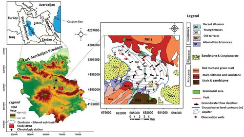
The prevailing climate in the Duzduzan plain is semi-arid–cold, as per classification by de Emberger (1930). Average annual precipitation is about 366 mm (Duzduzan climatological station, 2007/16). Mean daily temperature at the Berezin climatological station varies from −5.8°C (in January) to 23.2°C (in August), with an annual temperature average of 8.6°C. In general, average monthly relative humidity at the Berezin climatological station is fairly high, ranging from 41.1% (in July) to 75.3% (in March).

The Duzduzan plain has formations from the Miocene to the Pleistocene period (see Fig. 1). Marine deposits of the Miocene are often composed of allochthone sediments with contrasting red conglomerate, white-to-yellowish and pink limestone, red sandstone, shale and marl. There are also gypsiferous layers mostly within the lower Miocene Formation and as such the Miocene Formation is significant in the hydrogeochemistry of the Duzduzan plain aquifer. Pliocene sediments, at the west and southeast of the plain, are limited to conglomerate deposits. Quaternary deposits are well developed in the basin. Alluvial deposits include old deposits composed of conglomerate with interbedded silt and clay in mountain flanks that are high-level terraces, but there are also young deposits. Figure 1 also shows several faults in the study area.

The aquifer in the Duzduzan plain is heterogeneous and unconfined, with an aquifer surface area of 60 km². Water demand in the plain is met mainly by abstractions from four springs, three traditional qanats and 152 withdrawal water wells. Due to the absence of basin management plans, three of the natural springs and qanats are already distressed, tending to become dry at critical times of the year. This has given rise to restrictive rules being set, imposing limitations on any further proposed withdrawal wells and reducing pumping rates, which are not often enforced. Based on pumping tests carried out in the plain by the East Azerbaijan Regional Water Authority (2001), transmissivity is high (150–200 m²/d) towards the northwest of Duzduzan and the alluvial terraces. Low transmissivity zones (25–50 m²/d) are at the east of the aquifer due to its thinness.

There are 15 OWs in the Duzduzan plain to monitor groundwater levels. Their locations are distributed over the entire region, as shown in Figure 1. Groundwater levels have been recorded by the East Azerbaijan Regional Water Authority since 2003. Monthly records at OW 1–8 go back for 10 years, but those at OW 9–15 have less than 8 years of records. Due to the agricultural and drinking water demands, high withdrawal rates around Duzduzan town produce a maximum cone of depression in this area. The rate of decline of groundwater levels is approx. 0.3 m per year (from 2003 to 2016) according to records in the Duzduzan OWs. Maximum seasonal variation is observed from October (the lowest groundwater level) at the end of the irrigation season to June (the highest groundwater level). The groundwater flow direction in the aquifer of the Duzduzan plain is mainly towards the northwest (Fig 1).

3 Methodology

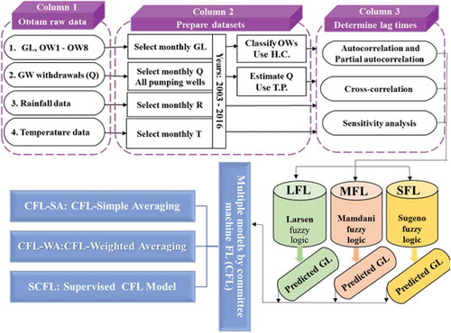
The models developed in this research work are schematized in Figure 2, which shows three FL models (SFL, MFL and LFL) at Level 1; their inherent information is extracted at Level 2 through three strategies of CM models: CFL, CFL-WA and CFL-SA. These methodologies are specified in this section without detailing them.

Figure 2. Flowchart illustrating the three FL models and three CM models used in the study.

3.1 Selecting model structures and preliminary data processing

Groundwater levels are modelled in this paper by developing FL models, which are used for time series analysis based on model structures in terms of the following input variables: lagged values of groundwater level (GL), discharge (Q), rainfall (R), temperature (T) and the output data comprise groundwater levels at observation wells. The study employs monthly mean values. In this section we present the model structure and argue that these models are essentially grey-box models.

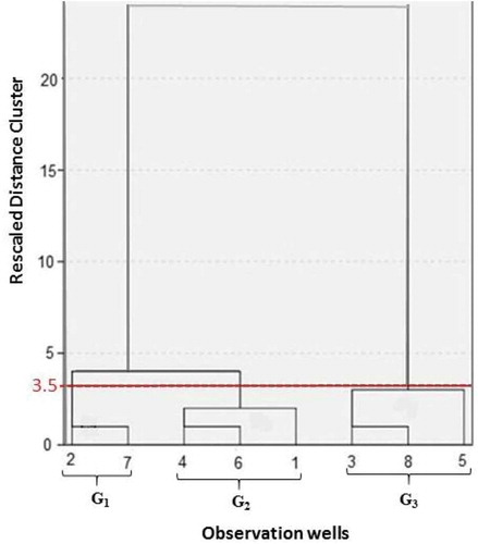
The monthly groundwater levels of the 15 OWs in the aquifer of the Duzduzan plain were parsed out and eight of them, which have the full data record, were selected to form the modelling dataset. The hierarchical clustering technique was used to classify the selected OWs to account for hydrogeological and morphological heterogeneity of the aquifer, based on their groundwater levels, elevation and altitude, as shown in Figure 3. This classification technique uses the Euclidean distance (or similarity measurement) between OWs and Ward’s method to apply the linkage rule (Ward 1963, Nadiri et al. 2013b). The water table level is important to ensure the hydraulic uniformity within each group and, as an example, OW 2 and 7 are in the same group. The threshold for the relative linkage distance is set to 3.5, but those shorter than 3.5 are classed in the same group. This threshold produces three groups: G1 (OW2 and OW7), G2 (OW1, OW4 and OW6) and G3 (OW3, OW5 and OW8) (see Fig. 3).

Figure 3. Classification of observation wells into groups using hierarchical clustering.

3.2 Fuzzy logic (FL) models at Level 1

Three FL models were used in this research; these make up the models at Level 1. These models establish relationships between a set of input data and a set of output data by building on the theory of fuzzy sets introduced by Zadeh (1965). This study did not use the first-generation FL models, which require prescribed rules. Instead, it used second-generation FL models, which are implemented through the identification of different clustering methods and learning the rules from the site-specific data, as detailed by Nadiri et al. (2017b, 2017c, 2018a). These use different clustering methods to identify clusters within the data and their optimum numbers (Chiu 1994). Three of the most widely used second-generation FL models are SFL, MFL and LFL, which are specified below.

Outputs of SLF are linear functions, which use the following: (a) constant or linear output membership functions, and called zero-order or first-order SFL, respectively (Sugeno 1985); and (b) SC is used to extract fuzzy If–Then rules (Chiu 1994, Chen and Wang 1999). In SC methods, the number of rules is equal to the number of clusters and is controlled by the clustering radius, which varies in the range of 0 and 1. The final output of the system is the weighted average of all rule outputs (aggregation), computed as follows:

(1) ${\widehat{\mathrm{G}\mathrm{L}}}_{\mathrm{O}\mathrm{u}\mathrm{t}}=\frac{\sum _{\mathrm{i}}{\mathrm{w}}_{\mathrm{i}}\widehat{\mathrm{G}\mathrm{L}}}{\sum _{\mathrm{i}}{\mathrm{w}}_{\mathrm{i}}}$(1)

where, ${\widehat{GL}}_{\mathrm{O}\mathrm{u}\mathrm{t}}$ is the final output of the fuzzy system, $w_i$ is the weight of the ith rule and $\widehat{GL}$ is the output of the ith rule.

MFL models are described as follows: (a) the output membership functions use the “Min” operation for their fuzzy implications (Mamdani 1977); and (b) rules are identified by the FCM clustering method (Newton et al. 1992, Lee 2004). LFL is similar to MFL except that LFL uses the product operator for the fuzzy implication operations (Larsen 1980).

It is noted that, for each group of OWs, their variables are entered in parallel but one model is fitted for each group of OWs and this contributes to model efficiency. The derived rules based on SC or FCM are data-driven rules, which may be contrasted with laws of nature or empirical formulas using laboratory or field tests. These data-driven rule bases are sufficient to call the models in this study grey-box models.

3.3 Committee fuzzy logic (CFL) models at Level 2

The multiple models approach is implemented by committee FL (CFL) models, and in this paper they are implemented as follows: Level 1 uses the above three models, SFL, MFL and LFL; Level 2 formulates CFL models, in which the outputs of the three Level 1 models are combined with the aim of reaping their benefits by employing the following: (a) simple averaging (SA), hence CFL-SA; (b) weighted averaging (WA), hence CFL-WA; and (c) supervised committee machines (SCM) running FL models, hence SCFL.

3.3.1 CFL-SA

This is a simple approach (Naftaly et al. 1997, Chen and Lin 2006), expressed as follows:

(2) $\mathrm{G}{\mathrm{L}}_{\mathrm{C}\mathrm{F}\mathrm{L}-\mathrm{S}\mathrm{A}}=\frac{1}{3}\mathrm{G}{\mathrm{L}}_{\mathrm{S}\mathrm{F}\mathrm{L}}+\frac{1}{3}\mathrm{G}{\mathrm{L}}_{\mathrm{M}\mathrm{F}\mathrm{L}}+\frac{1}{3}\mathrm{G}{\mathrm{L}}_{\mathrm{L}\mathrm{F}\mathrm{L}}$(2)

3.3.2 CFL-WA

In this approach the values of CFL-WA are modelled as:

(3) $\mathrm{G}{\mathrm{L}}_{\mathrm{C}\mathrm{F}\mathrm{L}-\mathrm{W}\mathrm{A}}=w_1\mathrm{G}{\mathrm{L}}_{\mathrm{S}\mathrm{F}\mathrm{L}}+w_2\mathrm{G}{\mathrm{L}}_{\mathrm{M}\mathrm{F}\mathrm{L}}+w_3\mathrm{G}{\mathrm{L}}_{\mathrm{L}\mathrm{F}\mathrm{L}}$(3)

where the values of $w_1$, $w_2$ and $w_3$ are identified by genetic algorithm (GA) through:

(4) $\mathrm{M}\mathrm{S}\mathrm{E}=\frac{1}{m}\sum _{i=1}^m{\left(w_1\mathrm{G}{\mathrm{L}}_{\mathrm{S}\mathrm{F}\mathrm{L}}+w_2\mathrm{G}{\mathrm{L}}_{\mathrm{M}\mathrm{F}\mathrm{L}}+w_3\mathrm{G}{\mathrm{L}}_{\mathrm{L}\mathrm{F}\mathrm{L}}\right)}^2$(4)

where GL is groundwater level, m is the number of training data points, and the sum of weights is unity $\left(\sum _i^m{w}_i=1\right)$. The mean square error (MSE) values are selected for the minimization by a GA optimizer (see Kadkhodaie-Ilkhchi et al. 2009, Labani et al. 2010).

3.3.3 SCFL

The SCM models introduced by Nadiri et al. (2013a) are also a model combination technique that overarches the three FL models by using ANN to extract the appropriate information for their combination. ANNs in these implementations use the multi-layer perceptron (MLP) for their feedforward processing and the Levenberg-Marquadt (LM) algorithm for their back-propagation operations (Baghapour et al. 2016).

The ANN model is processed as follows:

• (a) the architecture of the MLPs comprises neurons at the input layer, hidden layer and output layers;

• (b) the number of neurons for the input and output layers is set by the model structure;

• (c) the topology of the hidden layer (number of neurons) is normally identified through a preliminary trial-and-error step;

• (d) input data are normalized and regarded as signals moving only in the forward direction; and

• (e) incoming signals are linearly combined and converted to input signals of the hidden layer by assigning activation functions (using the nonlinear sigmoid transfer function in the hidden layer and transfer input signals to the output layer).

SCFL is expressed mathematically as follows:

(5) ${\mathrm{O}\mathrm{u}\mathrm{t}}_i^{\mathrm{F}\mathrm{L}}={\mathrm{F}\mathrm{L}}_i\left(\mathrm{G}{\mathrm{L}}_{\mathrm{t}-2},Q_{t-1},R_{t-1},T_{t-1}\right)$(5)

(6) $O_j=f_1\left(b_j+\sum _i{W}_{ij}{\mathrm{O}\mathrm{u}{\mathrm{t}}_{\mathrm{i}}}^{FL}\right)$(6)

(7) ${\widehat{\mathrm{G}\mathrm{L}}}_{\mathrm{S}\mathrm{C}\mathrm{F}\mathrm{L}}=O_k=f_2\left(b_k+\sum _j{W}_{kj}{O}_j\right)$(7)

where, ${\mathrm{O}\mathrm{u}\mathrm{t}}_i^{FL}$ is output from each FL model (i = 1: SFL; i = 2: MFL; i = 3: LFL); $f_1$ is the transfer function for the hidden layer (hyperbolic tangent sigmoid – tansig); $f_2$ is the transfer function for the output layer (linear – Purlin); $O_j$ is the jth output of nodes in the hidden layer; $W_{ij}$ and $W_{kj}$ are weights to control the strength of connections between two layers; $b_i$ and $b_k$ are bias values used to adjust the mean value for the hidden layer and output layer, respectively; t is time; and, finally, the lags associated with each GL variable in the grey-box model are discussed in due course. The weights $W_{ij}$, $W_{kj}$ and biases are identified by the LM algorithm.

3.4 A mathematical insight into SCFL models

The premise on which the CFL models learn from MMs has a mathematical basis as outlined below. There are M trained multiple models (three FL in this paper): ${\mathrm{G}\mathrm{L}}_m^{\mathrm{F}\mathrm{L}}$, to predict the observed groundwater levels ($\mathrm{G}{\mathrm{L}}_{\mathrm{o}\mathrm{b}\mathrm{s}}$). The prediction error is written as:

(8) $e_{m,i}={\mathrm{G}\mathrm{L}}_{m,i}^{\mathrm{F}\mathrm{L}}-\mathrm{G}{\mathrm{L}}_{\mathrm{o}\mathrm{b}\mathrm{s},i}$(8)

where $m=1,\dots ,M$ (in which M = 3).

The expectation of the squared error for the ith fuzzy model for a given m (${\mathrm{G}\mathrm{L}}_{m,i}^{\mathrm{F}\mathrm{L}})$is:

(9) $E_{m,i}=\epsilon \left[\left({\text{GL}}_{m,i}^{\text{FL}}-{\text{GL}}_{\text{obs},i}{)}^2\right)\right]=\epsilon \left[e_{m,i}^2\right]$(9)

In which $\epsilon \left[.\right]$ is the expectation and i = 1, N, where N is number of data points. The average error for each of the fuzzy models used alone is:

(10) $E_{\mathrm{a}\mathrm{v}\mathrm{g},\mathrm{m}}=1/N\sum _{i=1}^N{\mathrm{E}}_{m,i}=\left(1/N\right)\sum _{m,i}^n\epsilon \left[e_{m,i}^2\right]$(10)

Applying the averaging method, output vector $\mathbf{G}{\mathbf{L}}_{m,i}$ of the CFL is:

(11) $\mathbf{G}{\mathbf{L}}_{\mathrm{C}\mathrm{F}\mathrm{L}}=1/M\sum _{m=1}^M{\mathrm{G}\mathrm{L}}_{m,i}^{\mathrm{F}\mathrm{L}}$(11)

Therefore, the CFL has the prediction-squared error:

(12) ${\mathrm{E}}_{\mathrm{C}\mathrm{F}\mathrm{L}}=\epsilon [(\mathrm{G}{\mathrm{L}}_{\mathrm{C}\mathrm{F}\mathrm{L}}-\mathrm{G}{\mathrm{L}}_{\mathrm{o}\mathrm{b}\mathrm{s}}{)}^2=\epsilon \left[{\left(1/M\sum _{m=1}^M{\mathrm{G}\mathrm{L}}_{m,i}^{\mathrm{F}\mathrm{L}}-\mathrm{G}{\mathrm{L}}_{\mathrm{o}\mathrm{b}\mathrm{s},i}\right)}^2\right]=\epsilon \left[{\left(1/M\sum _{m=1}^M{e}_m\right)}^2\right]$(12)

Considering Cauchy’s inequality:

(13) ${\left(a_1{b}_1+a_2{b}_2+\cdots +a_n{b}_n\right)}^2\le \left(a_1^2+a_2^2+\cdots +a_n^2\right)\times \left(b_1^2+b_2^2+\cdots +b_n^2\right)$(13)

and applying it to the $E_{\mathrm{C}\mathrm{F}\mathrm{L}}$ one obtains:

(14) $E_{\mathrm{C}\mathrm{F}\mathrm{L}}=\epsilon \left[{\left(1/N\sum _{i=1}^N{e}_{\mathrm{i}}\right)}^2\right]\le 1/N\sum _{i=1}^N\epsilon \left[e_{\mathrm{i}}^2\right]=E_{\mathrm{a}\mathrm{v}\mathrm{g}}$(14)

which indicates that the CFL gives smaller errors than the average of all the fuzzy models. Equation (14) was presented by Chen and Lin (2006) and Kadkhodaie-Ilkhichi et al. (2009); it indicates that the error by CFL should be smaller than that by the individual FL models. In this paper, we show an instance in which Equation (14) may not hold if observed values are outside the collective range of the individual models.

4 Building models and setting up datasets

The grey-box model developed in this study comprises three FL models and three CFL strategies, each producing a model; hence six models are built for each group of OWs, as follows.

4.1 Data availability and model structure

Four sets of raw data are used in this study and comprise: groundwater level (GL) records available for the three groups of OWs (see Section 3.1); discharge (Q), which quantifies withdrawals from the aquifer; rainfall (R) to set aquifer recharge; and ambient temperature (T), which is a measure of evaporation affecting groundwater.

The monthly record of groundwater levels at the OWs goes back to 2007, and this study uses the data for a period of 10 years (2007–2016). These data were supplied by the East Azerbaijan Regional Water Authority, which also supplied the raw data for discharge, rainfall and temperature. Overall, there were 26 missing data points in the records of GL. The quadratic spline fitting method was selected to estimate these missing values. Samples of groundwater levels are presented later in the paper (see Section 5). Notably, groundwater levels and withdrawals vary at each OW, but rainfall and temperature do not vary significantly from one OW to another.

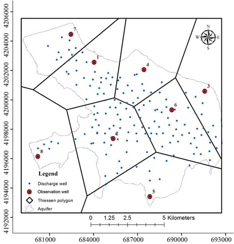
In spite of the classification of the OWs in the study area using the hierarchical clustering method, the calculation of the total withdrawal from an aquifer requires the use of the record available at each and all OWs. The monthly groundwater withdrawal for each OW was estimated using the Thiessen polygon method, thereby integrating the withdrawals from all of the individual abstraction wells within each polygon, as shown in Figure 4. Likewise, the aquifer was divided into eight zones (Fig. 4), as one polygon per OW. Approximately the first 80% of the time series data were used for model training (2007–2014) and the remaining data (2015–2016) for model testing.

Figure 4. Aquifer zones created using the Thiessen polygon method.

The monthly rainfall data were acquired from the Duzduzan rainfall station located about 75 km southeast of Tabriz for the 10-year period 2007–2016. The monthly maximum and minimum ambient temperatures for the 2007–2016 period were collected from the Berezin meteorological station, East Azerbaijan, Iran.

The selected model structure is a regression-type relationship, which expresses GL in terms of its own value lagging behind and the three parameters Q, R and T, where the selection is concerned with identifying those variables that make significant contributions to predicted groundwater levels. The procedure for the selection of model structure comprises: (a) sensitivity analysis, (b) statistical analysis in terms of cross-correlation, autocorrelation and partial autocorrelation techniques, and (c) checking rules of thumb; these are outlined below. In this paper it was considered sufficient to outline the processes without presenting detailed results.

4.1.1 Sensitivity test

Sensitivity analysis was carried out, similar to Shiri and Kisi (2011), for each OW by systematically removing each input dataset and checking the performance of the model. In this way, the optimum lag time of input data was indicated to be 1 month, and this value was set for each of the input GL Q, R, T variables.

4.1.2 Statistical tests

The dependency of each variable on previous values was tested through autocorrelation and partial autocorrelation, which showed that it takes up to 3–12 months for the dependence on the previous values to diminish to almost zero. The above two approaches lead to conflicting choices and therefore the choice of 1 month is difficult to justify, but this decision also depends on the parsimony of the model structure. The lag time of 1 month is therefore justified on the grounds of parsimony of the model structure, which takes a view of the available data (10 years of monthly readings, which makes 120 data points) and the number of parameters in each model, as presented in the next section.

4.2 Performance evaluation of the models

To examine the effectiveness of the models in predicting groundwater levels, the performance measures were quantified for all models using the following two metrics: root mean squared error (RMSE) and coefficient of determination (R²), which measure overall goodness of fit between the modelled and observed values. The closer the value of RMSE is to 0, the more accurate the prediction is. Notably, minimized RMSE, also used for specific purposes, behaves similar to RMSE. The coefficient of determination ($-1\le R^2\le 1$) describes the proportion of the total variance in the observed data that can be explained by the model. High $R^2$ values indicate better agreements between predicted and observed values (Legates and McCabe 1999).

5 Results

The water table is spatially distributed and therefore groundwater level recordings at the OWs were divided into three groups, each fitted with SFL, MFL and LFL, for which the variable values at each observation well were entered in parallel. These were used further to formulate three committee models of CFL-SA, CFL-WA and SCFL (giving six sets of modelling results for each group of OWs).

5.1 Prediction of groundwater level by fuzzy logic models

Cluster radii and the number of clusters, and thereby rules, were identified for each of the three FL models at each group of OWs.

5.1.1 Clusters and rules using SFL

The SFL models were implemented for each of the three groups of OWs (G1, G2 and G3) using the subtractive clustering (SC) technique by systematically increasing the cluster radii from 0 to 1. Consider the G1 group (comprising OW2 and OW7): its clustering radius (CR) was identified to be 0.5 by minimizing RMSE (see Fig. 5(a)). The input and output clusters were created using the triangular and linear membership functions, respectively. The number of If–Then rules was the same for the input data clusters, which were categorized in four clusters for the G1 observation wells. Full details for G1, G2 and G3 group are shown in Figure 5 for SFL, as well as for MFL and LFL, where the latter are identical.

Figure 5. The number of clusters (NC), clustering radius (CR) and number of rules (NR) based on minimum RMSE for three groups of OWs: (a) SFL and (b) MFL.

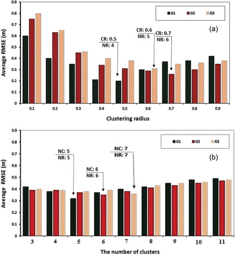
Based on minimized RMSE, the following clustering results were obtained for the SFL model: (a) four rules were identified for G1 and these rendered an optimum CR value of 0.5; (b) five rules were identified for G2, which rendered an optimum CR value of 0.6; and (c) six rules were identified for G3, with an optimum CR value of 0.7. The number of rules depends on the complexity of the input data and monthly variations of groundwater table in the OWs, which are highly variable.

The number of parameters, as discussed above, is a measure of the degrees of freedom in the subsequent model structure, according to which the number of unknowns is easily calculated. For instance, for G1 wells, the above cluster analysis assumes that the lag time is 1 month, according to which there are six inputs: four clusters, a triangular MF with inputs having two unknown parameters, and a linear MF with outputs for each rule having seven unknown parameters; this renders 86 parameters (6 × 4 × 2 = 72; 72 + (7 × 2) = 62). Similar numbers are rendered for the other group of wells, as 107 (G2) and 123 (G3). These have the same order of magnitude of the data points (168), as discussed in Section 4.1. Any greater selection of the lag time would therefore make the model overfitted, and hence the choice of 1 month for the lag time is justified, as the most plausible compromise.

5.1.2 Cluster and rules using MFL and LFL

These models were implemented for each of the three OW groups (G1, G2 and G3) using the fuzzy C-Mean (FCM) clustering method to extract the clusters and fuzzy rules. In this step, the optimum number of If–Then rules was identified by trial-and-error approach. The number of If–Then rules was the same for the input and output data clusters, as shown in Figure 6(b). Based on minimized RMSE, the following clustering results were obtained for the MFL and LFL models: five rules were identified for G1, six rules were identified for G2, and seven rules were identified for G3, The number of rules depends on the complexity of the input data and monthly variations of groundwater table in the OWs, which are highly variable. Notably, the lag time for both MFL and LFL were set to 1 month, as for SFL.

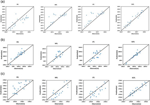
Figure 6. Scatter diagrams of measured vs modelled GL values – testing phase: (a) OW2 in G1, (b) OW4 in G2 and (c) OW8 in G3.

5.2 Performance of FL models at Level 1

5.2.1 Training results

The SFL, MFL and LFL models were built in three groups for predicting the groundwater levels at OW1–OW8 using the training data. The performance measures for each of the three models at each of the OWs are summarized in Table 1(a). According to Table 1, among the three FL models, SFL performs better than MFL and LFL in terms of all of the performance measures, but MFL and LFL have mixed results, as there are cases in which MFL may be poorer than LFL. Overall, both MFL and LFL are fit for purpose on the grounds of their performance metrics and therefore were used in further learning from their multiple models.

Table 1. Performance measures for the different models at observation wells OW1–OW8 in training and testing steps. Values in bold indicate the best performance; shaded figures indicate poor performance.

Statistical indicator	Model	OW1	OW2	OW3	OW4	OW5	OW6	OW7	OW8
(a) Training
RMSE (m)	SFL	0.198	0.14	0.364	0.302	0.315	0.257	0.187	0.187
	MFL	0.232	0.179	0.394	0.242	0.395	0.412	0.409	0.242
	LFL	0.256	0.220	0.374	0.274	0.377	0.399	0425	0.253
	CFL-SA	0.112	0.149	0.275	0.153	0.313	0.235	0.280	0.156
	CFL-WA	0.101	0.100	0.237	0.130	0.267	0.189	0.175	0.123
	SCFL	0.087	0.094	0.132	0.107	0.198	0.104	0.160	0.062
R^2	SFL	0.906	0.860	0.890	0.834	0.855	0.804	0.880	0.937
	MFL	0.803	0.751	0.907	0.800	0.825	0.874	0.860	0.831
	LFL	0.781	0.745	0.610	0.802	0.688	0.510	0.870	0.768
	CFL-SA	0.927	0.860	0.932	0.915	0.893	0.873	0.940	0.974
	CFL-WA	0.937	0.870	0.935	0.964	0.901	0.897	0.980	0.976
	SCFL	0.971	0.935	0.963	0.968	0.940	0.937	0.960	0.983
(b) Testing
RMSE (m)	SFL	0.282	0.272	0.416	0.358	0.315	0.342	0.211	0.198
	MFL	0.323	0.352	0.402	0.387	0.383	0.421	0.406	(0.242)
	LFL	0.390	0.401	0.420	0.301	0.482	0.429	0.478	(0.253)
	CFL-SA	0.221	0.237	0.305	0.222	0.322	0.333	0.332	0.192
	CFL-WA	0.202	0.185	0.241	0.201	0.302	0.280	0.202	0.173
	SCFL	0.135	0.115	0.187	0.176	0.252	0.198	0.198	0.103
R^2	SFL	0.882	0.704	0.800	0.613	0.721	0.748	0.673	0.662
	MFL	0.734	0.638	0.590	0.658	0.620	0.593	0.589	0.789
	LFL	0.813	0.602	0.612	0.612	0.491	0.661	0.569	0.734
	CFL-SA	0.863	0.814	0.851	0.890	0.773	0.803	0.698	0.890
	CFL-WA	0.895	0.824	0.858	0.910	0.842	0.770	0.682	0.915
	SCFL	0.920	0.925	0.883	0.935	0.870	0.897	0.690	0.940

5.2.2 Testing results

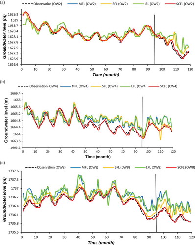
The performances of the three FL models in the testing phase were evaluated using the two performance measures, as for training the models, and the results obtained are summarized in Table 1(b), which confirms the results for the training phase. Scatter diagrams are presented in Figure 6 for OW2, OW4 and OW8, according to which SFL has slightly narrower scatter than MFL and LFL. Figure 7 shows time plots at OW2, according to which SFL initially reproduces observed values fairly well but gradually develops phase errors; this error amplifies with MFL and LFL. This is attributed to using the lag time of 1 month, but selecting any finer resolution would severely amplify computational costs and encourage overfitting. Overall, both MFL and LFL are fit for purpose to be used as multiple models on the grounds of their performance metrics.

Figure 7. Time plots of groundwater levels of individual FL and SCFL models in the testing and training phases for (a) OW2 in G1, (b) OW4 in G2 and (c) OW8 in G3.

The 45-degree line in each of the scatter diagrams shows the perfect fit and readily indicates the trend for overestimation or underestimation. Thus, the results show that for OW2 MFL and LFL models tend to overestimate, but SFL tend to underestimate and for OW8 MFL and LFL tends to underestimate, but SFL tend to overestimate and both are prone to scattering the results.

5.3 Preparation of multiple models at Level 2

The CFL-SA required no preliminary model processing but CFL-WA was implemented by developing a GA model through Equation (4) to identify the values of the weights from the data by minimizing MSE values. The default values in the implementation of the GA model are given in Table 2, which also shows that the highest weights were obtained for SFL at all the observation wells and the lowest weight for LFL at all of the observation wells except for OW3, OW5 and OW6. This indicates that poorer performance of LFL was mostly observed at OW1, OW2, OW4, OW7 and OW8. Notably, the order of weights of the three FL models is the same as the order of RMSE of the models.

Table 2. Optimized weights of different FL models by GA at each observation well (OW). G1–G3: groups 1–3.

Observation well	FL model
	SFL	MFL	LFL
OW1 (G2)	0.38	0.32	0.29
OW2 (G1)	0.48	0.28	0.23
OW3 (G3)	0.34	0.32	0.33
OW4 (G2)	0.46	0.29	0.25
OW5 (G3)	0.38	0.30	0.32
OW6 (G2)	0.44	0.27	0.28
OW7 (G1)	0.53	0.24	0.23
OW8 (G3)	0.42	0.32	0.26
	Highest weights	Lowest weights

GA uses the following initial default settings:

• population size (for three objective functions): 45;

• maximum number of generations: 180; mutation probability: 0.001–0.01;

• reproduction mechanism: roulette wheel;

• basis of chromosome selection: mean square error (MSE);

• cross-over type: two-points; mutation type: uniform; and cross-over probability: 0.8.

The SCFL was implemented by running an ANN (MLP-LM) model, in which input data layers were fed by the outputs of the SFL, MFL and LFL models. The structure in the MLP-LM model was identified through preliminary modelling by a trial-and-error procedure, according to which the following MLP topologies were identified: for G1: 6-4-2, for G2: 9-6-3, and for G3: 9-6-3. The transfer function for the hidden layer is TANSIG and the transfer function for the output layer is PURLIN.

5.4 Results by multiple models at Level 2

The SA method is the basic committee machine in multiple modelling, where each of the inputs has equal weights. However, the WA method is a more sophisticated committee machine, where the optimum combination of weights is obtained by an optimization method (by using GA). The multiple modelling by SCFL goes beyond that of CFL-WA and directly learns the connectivity from the input and output data. The training and testing results are given in Figure 7, which show that these three models improve on the performance of the individual FL models, in which the level of improvement by SCFL is significantly higher than those of the other two, and that of CFL-WA is notably higher than that by CFL-SA.

The results in Figure 7 and Table 1 show that the expected deterioration in the quality of performance measures from the training to the testing phases reduced for all of the modelling results.

5.5 Comparison of SCFL with CFL and FL models

The results in Table 1(a) for all the observation stations in the training phase show that SCFL performed consistently better than the individual FL models and better than CFL-SA and CFL-WA. The improvements by SCFL are significant, but CFL-SA and CFL-WA models still had notable improvements, in which CFL-WA performed better than CFL-SA for all observation wells. The scatter diagrams presented in Figure 6 for OW2, OW4 and OW8 indicate that the scattering in the data points was narrowed significantly. Phase errors in the time plot of groundwater levels are attributed to setting the lag time to 1 month, as explained above.

The results in Table 1(b) for all the observation stations in the testing phase show that SCFL performed consistently better than the individual FL models and better than CFL-SA and CFL-WA. The overall behaviour in this phase is similar to that of the training phase, as depicted in Figures 7 and 8, except that the drop in the quality of the performance measures from the training to the testing period was noticeable but expected. In particular, the phase error in Figure 7 is attributed to the lag time of 1 month.

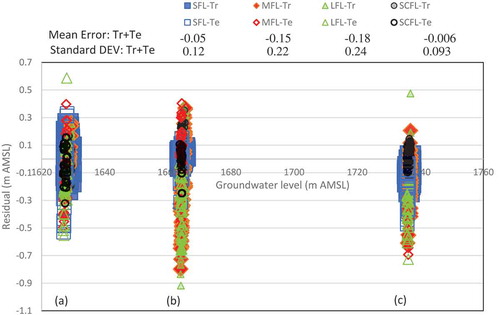
Figure 8. Scatter diagram of residuals (observed – modelled) vs observed groundwater levels for training (Tr) and testing (Te) phases at (a) OW2 in G1, (b) OW4 in G2 and (c) OW8 in G3. SCFL is represented by a black circle with the narrowest band and symbol sizes for SFL are exaggerated.

The study of performance measures in the results of the previous section provides quantitative evidence that the three FL models (SFL, MFL and LFL) produce fit-for-purpose results; the SFL model performs better than MFL and LFL in both the training and testing phases; and the MFL and LFL models have mixed fortunes with respect to both performance measures and the location of the OWs. The authors’ experience with other problems is that the issue of mixed fortunes in model performance does not follow any rule, but for each problem the quality of fit is a matter of learning. Similar studies of performance measures of CM models indicate that SCFL, CFL-WA and CFL-SA produce further improvements; the improvements by SCFL are remarkably better than those of the other MM alternatives; and phase errors are observed with CFL-WA and CFL-SA.

As expected, the predicted values differ from their corresponding observed values, and a visual comparison of the observed and predicted GL values is displayed in Figure 7 as time plots of groundwater levels for OW2. Based on Figure 7, the following information is extracted: all six time plots reproduce observed values, but to varying degrees of accuracy; (ii) other than LFL, each model reproduces observed GL rather accurately for more than a year of the 3 years in the testing period, but phase errors creep in from there on; and (iii) LFL suffers a noticeable level of phase error. Traditional model selection practices seek best performing models and, as such, the tendency would be to rank the models (SFL, MFL and LFL or SFL, LFL and MFL), whereas this study focused on learning from SFL, MFL and LFL.

6 Discussion

The models developed in this study provide insight into a range of issues, as discussed below, which confirms the confidence in the developed models and thereby their application to study a number of management issues.

6.1 An observed problem in multiple models

Attention is drawn to an anomaly observed in the performance of CFL-SA at OW4, where the RMSE for CFL-SA was higher than that of the mean of SFL, MFL and LFL (see Table 1(a)). Based on the mathematical proof presented for Equation (14), previous researchers (Kadkhodaie-Ilkhichi et al. 2009, Labani et al. 2010, Nadiri et al. 2013a, Fijani et al. 2013, Nadiri et al. 2015b), hold that the RMSE obtained by SA should be less than the mean RMSE of the individual models. Thus, the above observation is in conflict with the proof reproduced in Section 3.3 through Equations (8)–(14). The authors have not cited a report on such an anomaly and therefore they examined the results and derivation of Equation (14). The examination indicated that the RMSE by SA or WA could fail to render improvements compared with the mean RMSE of the individual models, contrary to the implications of Equations (8)–(14). This paper sheds light on the problem that the application of CFL-SA and CFL-WA should produce improvements if their results and their corresponding observed values are within the range of the maximum and minimum values of the single models. Notably, SCFL is successful even in this adverse case without any additional conditions.

6.2 Quality of model fitting

The clustering techniques used by the three FL models are intrinsically parsimonious, and the selected models satisfy the diminishing return problem (see Nadiri et al. 2017a) for a further detail, although there is a risk of underfitting, as discussed above, due to the monthly resolution of the data or their record length. A similar problem prevails in selecting the topology (i.e. the number of hidden layers) of ANN models, where too few neurons in the hidden layer is called underfitting, while the problem suffers from overfitting when there are too many neurons. In practice, the parsimonious topology is selected through a trial-and-error procedure and with further examination of the model structure. In this study, the selection of 1 month for the lag time ensures that the model is not overfitted but exposes the results to underfitting. The data record (14 years) is not long enough to warrant the exploration of a more sophisticated topology and therefore the lag time of 1 month is justified for this study, as any greater topology would create interactions with the FL models or lead to overfitting. Nonetheless, an examination of the results indicates some phase error, attributable to underfitting.

To the best knowledge of the authors, there is no past work in modelling aquifers using bottom-up AI techniques with two levels of learning and therefore no comparison with reported studies is possible. A collective view is also reflected in that two levels of learning in AI modelling practices marks a shift in modelling cultures, as discussed in greater depth by Khatibi et al. (2017). In the prevailing culture, alternative models or algorithms are developed and compared in search of a superior model for an exclusive ranking at the expense of the others, but use anecdotal case studies without much critical view of the practice. However, learning at two or more levels departs from existing practices and puts the emphasis on learning, and this is the culture of inclusion in modelling practices, which promotes learning at every opportunity. However, both practices rely on “shallow” performance metrics, which provide system-wide measures of goodness of fit. One way of penetrating into the actual performance is a study of residuals, as presented in Figures 7 and 8. Another way is to develop a risk-based approach, in which accuracy would be defined in terms of significant sensitivity to revealing risk bands. However, insufficient data are available for the study area, as it would also require social and land-use data.

6.3 Grey-box models

The theoretical basis for the models developed in this paper falls under the grey-box models, which lie between black-box and white-box models. Black boxes or regression-type models connect input and output variables by a mathematical strategy without treating the underlying processes. Grey boxes make further allowances for the underlying processes by developing If–Then rules. The rules are derived using a strategy such as FL by learning from the data by the fully objective clustering techniques. Notably, similar procedures were used by Alvisi et al. (2006) using SFL and MFL models.

6.4 Applications

Examining residuals reveals further information about the nature of the errors. Therefore, time plots of residuals against observed groundwater levels are used to study possible trends in the data, where residuals are defined in terms of the differences between simulated and observed groundwater levels. The residuals are dependent on: (a) measurement errors, which are often random; and (b) modelling errors, which can be much more complex. However, if the residuals reflect randomness, they rule out the existence of possible trends in the data. These results are displayed in Figure 8 for three observation wells OW2, OW4 and OW8. The problem is that a compact representation of the results leads to squashing the distribution of the data points, but these provide visual evidence that there is no trend in the residuals of the SCFL model as they are in a narrow band and narrower than those for SFL, MFL and LFL. However, the low-resolution plots in Figure 8 are associated with the metrics of mean error and standard deviation of each of the four models (SCFL, SFL, MFL and LFL) and those of SCFL are closer to zero. The highest dependency of the residuals on observation values is related to MFL and LFL models with one level of learning. Similar studies were also carried out by Jha and Sahoo (2015).

The relative importance of withdrawal and rainfall in terms of groundwater levels is evaluated by a sensitivity study of management goals through the following two scenarios for the Duzduzan aquifer: (a) increase monthly rainfalls by 10% to emulate aquifer recharge; and (b) decrease monthly withdrawal by 10% to emulate a surge in demand. The first scenario can be thought of as relating to emulating climatic impacts and the second to emulating anthropogenic impacts on water demand. Both of these scenarios may help to recover water table delineation in this aquifer. The test results based on SCFL are presented in Figure 9, which reveals that water use has higher impacts on water table variations in this aquifer than possible climatic changes such as rainfall. Thus, recovery of the water table in the study area is more sensitive to abstractions than to recharges, and this provides evidence to show the need for a planned management of the study area.

Figure 9. Sensitivity studies to identify the factors contributing to the recovery of water tables: (a) SCFL results for OW2 at G1, (b) SCFL results for OW1 at G2, (c) SCFL results for OW3 at G3.

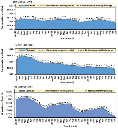
Watercourses within the Duzduzan plain are ephemeral and this signifies the important role of groundwater in meeting water demand for drinking, industry and irrigation in this region. In recent years, abstraction of groundwater resources has been intensified by increased pumping across the plain, and this is a primary source of an emerging decline in groundwater levels as well as in the deterioration of water quality. The research reported herein provides basic insights for the development of basin management plans and water cycle studies: (a) to reduce the decline of water resources within the plain; (b) to identify water saving measures and overhaul traditional irrigation systems for more water saving agricultural practices; and (c) to set appropriate pumping rules, which are equitable and, as such, essential for enforcing the rules. Note that the response to a 5% decrease in withdrawal at OW3 does not render proportional recovery in the water table as in the other OWs; this is because the number of withdrawal wells within this polygon is significantly lower than in the other polygons.

The model is also used to back-calculate specific yield at each polygon of OWs, where this is normally measured using costly measurements of constant pumping rate. Back-calculations using existing constant pumpage rate for the Duzduzan aquifer suggest the average specific yield of the aquifer to be approximately 4%. The model is used to estimate, but this value can now be estimated from the model for each polygon in terms of the increase in GL caused by its corresponding decrease in the withdrawal volume at each polygon. Using the model, the average estimated specific yield values for G1, G2 and G3 are given in Table 3. Note the proximity of the values within each OW group, which substantiates the results from hierarchical clustering.

Table 3. Specific yield at each OW – estimated.

Group	Observation well	Estimated specific yield (%)	Estimated average specific yield (%)
G1	OW2	4.7	4.8
	OW7	4.9
G2	OW1	3.9	3.7
	OW4	3.6
	OW6	3.7
G3	OW3	3.4	3.2
	OW5	3.2
	OW8	3.1

7 Conclusions

This research addressed a typical case of the need for modelling water tables of aquifers and studying their temporal variation where data are sparsely available. Groundwater levels in the study area were predicted by three FL models: Sugeno (SFL), Mamdani (MFL) and Larsen (LFL). Performance measures of these models indicate that their results are not identical; their ranking is only significant to local data; although the results are fit-for-purpose and so they are used in the next level of modelling for further learning.

The results of the three FL models were combined to form multiple models, referred to as committee FL (CFL) models, for further extracting information from the convergence and divergence between the modelling results. Three sets of MM modelling results were investigated: (a) CFL with simple averaging (CFL-SA); (b) CFL with weighted averaging (CFL-WA), in which the weights are derived using a genetic algorithm (GA); and (c) supervised committee FL (SCFL) models, in which an artificial neural network (ANN) runs the three models SFL, MFL and LFL to extract further information. The three SC models produced further improvements, in which SCFL performed better than the other models, with mixed fortunes, but still good enough. The improvement by SCFL is significant and its results closely replicate their corresponding measured values; as such it reveals no trend in terms of the residual errors (modelled minus observed values plotted against their corresponding groundwater levels).

The paper innovates in extracting further information by forming multiple models from existing models and the subsequent approach is reliable enough to carry out sensitivity tests and gain an insight into the behaviour within the local data. The results may be anecdotal; however, two issues can be underlined: (a) learning from the local data is important though not transferrable to other sites; and (b) the developed methodology is generic and can be applied to any aquifer system. Also, the research reported in this paper provides basic insights for the development of basin management plans and water cycle studies: (i) to reduce the decline of water resources within the plain; (ii) to identify water saving measures and overhaul traditional irrigation systems for more water saving agricultural practices; and (iii) to set appropriate pumping rules, which are equitable and can be enforced.

Acknowledgements

The authors wish to express their gratitude to the East Azerbaijan Regional Water Authority for providing the data for this research.

Disclosure statement

No potential conflict of interest was reported by the authors.

Additional information

Funding

This research is one of the outputs of the Artificial Intelligence Multiple Models research group, which is financially supported by the University of Tabriz through a grant scheme.

References

- Alvisi, S., et al., 2006. Water level forecasting through fuzzy logic and artificial neural network approaches. Journal of Hydrology and Earth System Sciences, 10 (1), 1–17. doi:10.5194/hess-10-1-2006
- Asadi, S., et al., 2014. Artificial intelligence modeling to evaluate field performance of photocatalytic asphalt pavement for ambient air purification. Environmental Science and Pollution Research, 21 (14), 8847–8857. doi:10.1007/s11356-014-2821-z
- Baghapour, M.A., et al., 2016. Optimization of DRASTIC method by artificial neural network, nitrate vulnerability index, and composite DRASTIC models to assess groundwater vulnerability for unconfined aquifer of Shiraz Plain, Iran. Journal of Environmental Health Science and Engineering, 14 (1), 13. doi:10.1186/s40201-016-0254-y
- Chen, C.H. and Lin, Z.S., 2006. A committee machine with empirical formulas for permeability prediction. Computers and Geosciences, 32 (4), 485–496. doi:10.1016/j.cageo.2005.08.003
- Chen, M.S. and Wang, S.W., 1999. Fuzzy clustering analysis for optimizing fuzzy membership functions. Fuzzy Sets and Systems, 103 (2), 239–254. doi:10.1016/S0165-0114(98)00224-3
- Chitsazan, N., Nadiri, A.A., and Tsai, F.T.-C., 2015. Prediction and structural uncertainty analyses of artificial neural networks using hierarchical Bayesian model averaging. Journal of Hydrology, 528, 52–62. doi:10.1016/j.jhydrol.2015.06.007
- Chiu, S., 1994. Fuzzy model identification based on cluster estimation. Journal of Intelligent & Fuzzy Systems, 2, 267–278.
- Daliakopoulos, I.N., Coulibaly, P., and Tsanis, I.K., 2005. Groundwater level forecasting using artificial neural networks. Journal of Hydrology, 309, 229–240. doi:10.1016/j.jhydrol.2004.12.001
- Emberger, L., 1930. Sur une formule applicable en g´eogrphiebotanique. Cahiers Herbs Seances de l’Academie des Sciences, 191, 389–390.
- Fijani, E., et al., 2013. Optimization of DRASTIC method by supervised committee machine artificial intelligence to assess groundwater vulnerability for Maragheh-Bonab plain aquifer Iran. Journal of Hydrology, 503, 89–100. doi:10.1016/j.jhydrol.2013.08.038
- Giustolisi, O. and Simeone, V., 2010. Optimal design of artificial neural networks by a multi-objective strategy: groundwater level predictions. Hydrological Sciences Journal, 53, 502–523.
- Jha, M.K. and Sahoo, S., 2015. Efficacy of neural network and genetic algorithm techniques in simulating spatio-temporal fluctuations of groundwater. Hydrological Processes, 29, 671–691. doi:10.1002/hyp.v29.5
- Kadkhodaie-Ilkhchi, A., et al., 2009. Petrophysical data prediction from seismic attributes using committee fuzzy inference system. Computers and Geosciences, 35, 2314–2330. doi:10.1016/j.cageo.2009.04.010
- Khatibi, R., Ghorbani, M.A., and Pourhosseini, F.A., 2017. Stream flow predictions using nature-inspired Firefly Algorithms and a Multiple Model strategy – directions of innovation towards next generation practices. Journal of Advanced Engineering Informatics, 34, 80–89. doi:10.1016/j.aei.2017.10.002
- Khatibi, R., et al., 2011. Comparison of three artificial intelligence techniques for discharge routing. Journal of Hydrology, 403, 201–212. doi:10.1016/j.jhydrol.2011.03.007
- Labani, M.M., Kadkhodaie-Ilkhchi, A., and Salahshoor, K., 2010. Estimation of NMR log parameters from conventional well log data using a committee machine with intelligent systems: a case study from the Iranian part of the South Pars gas field, Persian Gulf basin. Journal of Petroleum Science and Engineering, 72, 175–185. doi:10.1016/j.petrol.2010.03.015
- Lallahem, S., et al., 2005. On the use of neural networks to evaluate groundwater levels in fractured media. Journal of Hydrology, 307, 92–111. doi:10.1016/j.jhydrol.2004.10.005
- Larsen, P.M., 1980. Industrial applications of fuzzy logic control. International Journal of Man-Machine Studies, 12, 3–10. doi:10.1016/S0020-7373(80)80050-2
- Lee, K.H., 2004. First course on fuzzy theory and applications. Berlin: Springer.
- Legates, D.R. and McCabe, G.J., 1999. Evaluating the use of “goodness-of-fit” measures in hydrologic and hydroclimatic model validation. Water Resources Research, 35 (1), 233–241. doi:10.1029/1998WR900018
- Mamdani, E.H., 1977. Application of fuzzy logic to approximate reasoning using linguistic synthesis. IEEE Transactions on Computers, 26, 1182–1191. doi:10.1109/TC.1977.1674779
- Mohanty, S., et al., 2013. Comparative evaluation of numerical model and artificial neural network for simulating groundwater flow in Kathajodi-Surua Inter-basin of Odisha, India. Journal of Hydrology, 495, 38–51. doi:10.1016/j.jhydrol.2013.04.041
- Nadiri, A.A., et al., 2013a. Supervised committee machine with artificial intelligence for prediction of fluoride concentration. Journal of Hydroinformatics, 15 (4), 1474–1490. doi:10.2166/hydro.2013.008
- Nadiri, A.A., et al., 2013b. Hydro geochemical analysis for Tasuj plain aquifer, Iran. Journal of Earth System Science, 122 (4), 1091–1105. doi:10.1007/s12040-013-0329-4
- Nadiri, A.A., et al., 2014. Bayesian artificial intelligence model averaging for hydraulic conductivity estimation. Journal of Hydrologic Engineering, 19, 520–532. doi:10.1061/(ASCE)HE.1943–5584.0000824
- Nadiri, A.A., et al., 2017a. Groundwater vulnerability indices conditioned by Supervised Intelligence Committee Machine (SICM). Science of the Total Environment, 574, 691–706. doi:10.1016/j.scitotenv.2016.09.093
- Nadiri, A.A., et al., 2017b. Assessment of groundwater vulnerability using supervised committee to combine fuzzy logic models. Environmental Science and Pollution Research, 24 (9), 8562–8577. doi:10.1007/s11356-017-8489-4
- Nadiri, A. A., et al., 2017c. Mapping vulnerability of multiple aquifers using multiple models and fuzzy logic to objectively derive model structures. Journal of Science of the Total Environment, 593, 75–90. doi: 10.1016/j.scitotenv.2017.03.109
- Nadiri, A.A., et al., 2018a. Hybrid fuzzy model to predict strength and optimum compositions of natural Alumina-Silica-based geopolymers. Computers and Concrete, 21 (1). doi:10.12989/cac.2018.21.1.000
- Nadiri, A.A., et al., 2018b. Prediction of effluent quality parameters of a wastewater treatment plant using a supervised committee fuzzy logic model. Journal of Cleaner Production, 180, 539–549. doi:10.1016/j.jclepro.2018.01.139
- Nadiri, A.A., et al., 2018c. Introducing the risk aggregation problem to aquifers exposed to impacts of anthropogenic and geogenic origins on a modular basis using “risk cells”. Journal of Environmental Management, 217, 654–667. doi:10.1016/j.jenvman.2018.04.011
- Nadiri, A.A., et al., 2018d. Mapping specific vulnerability of multiple confined and unconfined aquifers by using artificial intelligence to learn from multiple DRASTIC frameworks. Journal of Environmental Management, 227, 415–428. doi:10.1016/j.jenvman.2018.08.019
- Nadiri, A.A., Asgharimoghaddam, A., and Shokri, S., 2015a. Efficiency assessment of wastewater treatment plant of Tabriz using artificial intelligence models. Journal of Environmental Studies, 40 (4), 827–844.
- Naftaly, U., Intrator, N., and Horn, D., 1997. Optimal ensemble averaging of neural networks. Journal of Computational Neuroscience, 8, 283–296.
- Nayak, P.C., et al., 2004. A neuro-fuzzy computing technique for modeling hydrological time series. Journal of Hydrology, 291 (1–2), 52–66. doi:10.1016/j.jhydrol.2003.12.010
- Newton, S.C., Pemmaraju, S., and Mitra, S., 1992. Adaptive fuzzy leader clustering of complex data sets in pattern recognition. IEEE Transactions on Neural Networks, 3, 794–800. doi:10.1109/72.159068
- Nourani, V., Mogaddam, A., and Nadiri, A.O., 2008a. An ANN-based model for spatiotemporal groundwater level forecasting. Hydrological Processes, 22, 5054–5066. doi:10.1002/hyp.v22:26
- Nourani, V., et al., 2008b. Forecasting spatiotemporal water levels of Tabriz aquifer. Trends in Applied Sciences Research, 3 (4), 319–329. doi:10.3923/tasr.2008.319.329
- Sahoo, M., et al., 2016. Space–time forecasting of groundwater level using a hybrid soft computing model. Hydrological Sciences Journal, 62, 561–574.
- Shiri, J. and Kişi, Ö., 2011. Comparison of genetic programming with neuro-fuzzy systems for predicting short-term water table depth fluctuations. Computers and Geosciences, 37 (10), 1692–1701. doi:10.1016/j.cageo.2010.11.010
- Sugeno, M., 1985. Industrial application of fuzzy control. New York: North-Holland.
- Tayfur, G., Nadiri, A.A., and Moghaddam, A.A., 2014. Supervised intelligent committee machine method for hydraulic conductivity estimation. Water Resources Management, 28, 1173–1184. doi:10.1007/s11269-014-0553–y
- Ward Jr., J.H., 1963. Hierarchical grouping to optimize an objective function. Journal of the American Statistical Association, 58, 236–244. doi:10.1080/01621459.1963.10500845
- Yurdusev, M.A., et al., 2009. Neural networks and fuzzy inference systems for predicting water consumption time series. Stochastic Environmental Research and Risk Assessment, 23, 1225. doi:10.1007/s00477-009-0320-4
- Zadeh, L.A., 1965. Fuzzy sets. Information and Control, 8 (3), 338–353. doi:10.1016/S0019-9958(65)90241-X