Application of lagged correlations between solar cycles and hydrosphere components towards sub-decadal forecasts of streamflows in the Western USA

ABSTRACT

Trade winds localized within the Western Equatorial Pacific express lagged and statistically significant correlations to sunspot numbers as well as to streamflow in rivers of the Southern Rocky Mountains. Both correlation sets were integrated in a linear regression analysis to produce relatively accurate sub-decadal streamflow forecasts for an annual and a 5-year average. In comparison to the autocorrelation technique, the prototyped method yielded the highest correlations, the highest goodness-of-fit scores, and the lowest root mean squared errors, for both the 5-year average and the annual average assignments. Of all of the cases examined, the highest Kolmogorov-Smirnov test scores between observation and prediction were found for the single solar-based forecast 5 years in advance for the 60-month average streamflow of the Animas River in New Mexico.

KEYWORDS:

• divergence of latent energy (LEDIV)
• circulation
• streamflow
• El Niño Southern Oscillation index (ENSO)
• Western Equatorial Pacific
• solar cycles

Editor A. Castellarin; Associate editor S. Kanae

Introduction

Much of surface hydrological practice relies upon stochastic approaches, which, in turn, depend on records of the history of a subject stream system for estimating that system’s future. Accordingly, the nominally predictive solutions are based on autocorrelation and/or autoregression moving average (ARMA) strategies, such as described in Wei (2006). These hydrological strategies are typically parametric, given that they are often geared to develop best estimates of the first several moments (mean, variance, skew) for a given time series or for a given seasonal subset. Those strategies are often further challenged by the difficulties of establishing what the actual underlying probability density function (pdf) or cumulative distribution function is, and for what periods they can apply. For example, Zeng et al. (2015) and Machiwal and Jha (2010) illustrate how different governing pdfs or related characteristics for selected streamflow or precipitation time series (for example, Pearson Type III versus normal or Weibull distributions) can be interpreted, simply by filtering out different seasons or other sub-populations for analysis. Without establishing the most appropriate pdf to employ, the calculated moments may not best serve the goals of estimating future conditions. Moreover, even if an estimate of a pdf were consistent, the resulting parameters would have limited utility in a forecasting role. Many parametric results are simply cast into climatological products, such as the mean flow for a given season or month, or as estimates of extreme events such as a probable maximum flood. A more desirable type of forecast for example might definitively project the arrival of a period of drought, with a certain lead time, span and intensity across a given region.

Accordingly, if independent and reliable precursors were available over various climatological time frames (multi-season to multi-decadal), then hydrologists would likely employ them in non-autocorrelation solutions towards improved forecasting. Precipitation is an obvious precursor candidate. Yet the phenomenon of atmospheric moisture itself is currently subject to the same limitations. Accordingly the autocorrelation method must typically be applied for that parameter as well, thereby compounding uncertainties.

Some independent precursors to regional climatological atmospheric moisture patterns have been described including the widely cited El Niño pattern, which itself is often lumped into a broader compendium of patterns termed the El Niño Southern Oscillation (ENSO) index (NOAA 2017¹). However, to date they have not proven to be consistently reliable for hydrological forecasting. Deterministic numerical global circulation models (GCMs) have also frequently been deployed towards these same forecast objectives, but none so far have been able to accurately simulate extended periods of integrated climate for the globe or any sub-region, at least with regard to hydroclimatology. Such models have also failed in hindcast exercises, where the prior and observed states are both known (Fricker et al. 2013).

With the goal of improving hydrological forecasting skill, researchers continue to experiment with the adoption of various combinations of selected precursors. Kalra et al. (2013), for example, utilized a statistical vector method in combination with the integration of a non-ENSO parameter mapped for the Western Pacific, known as the Hondo. Their method was applied with this added precursor to forecast streamflows within selected watersheds of the Western USA. One gage was close to a stream of the current study but monitored a stem tributary of the San Juan River just below a major reservoir in New Mexico. According to their study, forecasting performance was improved over the standard regression and other approaches.

In another example, Wang et al. (2010) investigated connections of the ENSO ensemble pressure parameter, known as the Southern Oscillation Index (SOI), to hydrological records of the Western USA. The SOI index identifies the surface pressure differential between Darwin, Australia, and Tahiti. The authors also compared their subject time series to the North Atlantic Oscillation (NAO), which is a temperature measure of the Atlantic in the Northern Hemisphere. Their subject hydrological time series was the lengthy water level record of the Great Salt Lake. The researchers noted the relatively dampened time signature of the water levels for that feature and suggested a connection to the SOI. Moreover, they identified similar quasi-decadal cycles within the various time series, and finally recommended that utilization of a 3-year lag might be effective for improved forecasting.

The above-mentioned studies searched alternate ocean patterns apart from favored ENSO indexes (namely the ONI index subset² ) as possible precursors to continental stream patterns. Aside from contemporary deterministic GCMs, most studies of this nature – whether or not ENSO based – have primarily focused on correlative structures. This paper utilizes some alternate indexes from the ENSO compendium in a correlative framework, and includes a somewhat greater emphasis on a specific causal notion. As opposed to the conventional adoption of precursors that are primarily temperature or pressure based, this paper focuses on those indexes that exemplify high masses of atmospheric moisture, along with related trade winds. Moreover, this work contemplates the possibility that solar radiant forcing can drive the underlying precursor parameters.

The Sun is indisputably the primary driver of our weather. However, explicit and physically consistent correlations between longer-term surface climate patterns and solar cycles, including the 11-year cycle (Schwabe 1844), have yet to be fully verified or widely documented. In contrast to this contemporary lack of evidence, older studies from the 19th and early 20th centuries produced extensive products that purported to show high correlations between solar cycles and climatic features, including, for example, global temperature estimates (Koppen 1914) and cyclone frequencies in the Indian Ocean (Meldrum 1885). Notably, the apparent persistence of these synchronous correlations had faded by the middle of the 20th century (Hoyt and Schatten 1997).

As introduced and surveyed in Appendices A1 and A2, new connections between the solar irradiance and climate signatures were identified in the upper atmosphere by the late 20th century. For example, Labitzke and Van Loon (1995) related solar cycles to filtered subsets of zonal atmospheric overturning data, such as the Quasi Biennial Oscillation (QBO). However, the establishment of near surface moisture and temperature correlations to sunspot number (SSN) has remained elusive to date. Many researchers have nonetheless recognized the potential to connect SSNs to surface water hydrology. This was considered a productive study area because streamflow records are commonly understood to represent an integrated signature of climate over their watershed footprint. Some researchers have accordingly explored possible relations of solar cycles to extreme streamflows, and/or seasonally filtered flows, often including additional data processing such as detrending. These strategies have led so far to mixed results within and between study regions and scopes.

For example a study of streams of western Canada explored the potential to use solar cycles as an aid in forecasting extreme flooding events (Prokoph et al. 2012). They found a strong 11-year cycle in maximum annual streamflow, particularly along the continental divide of the Rocky Mountains within their study domain. They concluded that higher SSN counts were associated with contemporaneous moisture deficits in that region. However, consistent correlations across their study domain and time series were not identified. An overlapping study by Fu et al. (2012) explored similarities in time series spectral signatures of streams throughout southern Canada with those of the solar cycle and El Niño through fast Fourier transforms and wavelet analyses. The paper asserted that correlations were statistically significant for subsets of the total population of streamflow records explored. Explorations of time lags or of averages other than annual averages were not emphasized, but the authors reported their interpretation that solar influences first impacted El Niño, which then impacted the Canadian streams of note. No forecasting exercises were included in either of these Canadian studies.

Somewhat better correlations to solar cycles were reported for the Parana River in South America (Mauas et al. 2008). A significant correlation (0.78) emerged after detrending and normalization operations were applied. Yet those correlations that were identified were found to be synchronous. Accordingly, there was no apparent lead time indicated between the solar signal and the streamflow signal, and therefore such a connection cannot likely be directly adapted for forecasting purposes, unless the solar signal itself can be reliably predicted.

In spite of limitations and shortcomings, several potentially useful relationships between solar fluctuations and changes in key Pacific Ocean and other hydroclimatological parameters are apparent, as illustrated by Figure 1(a). To facilitate comparison in this chart and several others between the wide variety of indexes, each time series has been normalized against its mean and standard deviation. The time series in this chart have also been detrended. They demonstrate among other things that a common decadal scaled local minimum can be identified for all featured indexes during the latter half of the 1970s. These indexes include the SSN, the Atlantic Multidecadal Oscillation (AMO), the Pacific Decadal Oscillation (PDO), the ENSO and the SOI,³ and streamflow records from the Ganges River⁴ in India and the Upper Pecos River⁵ (PnP) in North America.

Figure 1. Time series of several oscillatory climate signatures: (a) normalized and detrended 11-year trailing averages, and (b) normalized 5-year trailing averages for items with highest Pearson’s CC to the AMO.

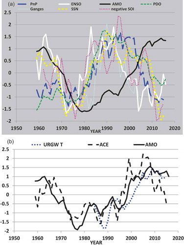
In exploring the time series of highest general correlations to solar cycles, a separate cluster of observations, which most strongly followed the AMO, has been developed and is shown in Figure 1(b). These observations include a temperature record (URGW T) taken from the European Reanalysis of Satellite Data (ERAI) datasets for the full atmosphere.⁶ In this example, the temperature is obtained from the Southern Rocky Mountain (SRM) zone featured in this study. The second record represents the accumulated cyclone energy (ACE) index.⁷ The correspondence between the ACE and AMO-related sea surface temperatures has been recognized by other researchers (e.g. Goldenberg et al. 2001). The manifold relationships between these variables and the latent heat patterns over the Pacific are naturally a subject of interest to many. These Atlantic connections are suggestive that temperature forecasting can potentially be improved to some extent, if a precursor to the AMO can be identified. However, given the focus of this paper on moisture forecasting, the topics related to Figure 1(b) are largely deferred to future examination.

Returning to the common minima feature of Figure 1(a), numerous additional concepts and correlations can be examined for potential improvements in regional hydroclimatological forecasting. Important background topics addressing the modern history of solar cycle connections to the atmosphere, along with a survey of potentially relevant published works on global moisture circulation principals, parameters and observations, are featured in the Appendix. Appendices A1–A3 have been organized to first summarize basic knowledge of global circulation patterns, followed by a brief survey of contemporary studies that explore connections between solar cycles and atmospheric time series, and, lastly, a review of quasigeostrophic (QG) features and their observed relations to atmospheric moisture and related parameters.

The Appendix is relied upon to develop a conceptual model in which the global hydrosphere undergoes energy changes over time and within its circulatory limbs, as a result, in part, of slight changes in the total solar irradiance (TSI) of approx. 0.17 W/m², on average. This irradiance anomaly is no more than 0.1% of the mean value, according to references found in Hoyt and Schatten (1997) and Gray et al. (2010). The TSI can be represented as an index in numerous variations, including the published monthly sunspot numbers (SSN) as archived at the Royal Observatory of Belgium, Brussels (WDC-SILSO).

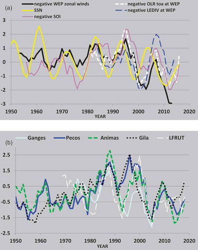
Within the context of information developed within Appendix A3, in particular, new correlations between solar cycles and atmospheric parameters have been found, as also represented in Figure 2(a). Figure 2(a) introduces the fact that, over the Western Equatorial Pacific (WEP) region, solar cycles, as indicated by SSN, express pervasive lagged correlations to multiple components of the atmosphere. As described in Appendix A3 and illustrated in Figure A2(a) and (b), these connections can be seen across that footprint from the surface, through the core, and up to the top of the atmosphere (TOA).

Figure 2. Normalized 5-year trailing average time series observations for non-continental and continental locations: (a) solar and Pacific Ocean atmosphere parameters, and (b) streamflow observations in the Himalaya and Rocky Mountain basins of the Northern Hemisphere.

The high-correlation solar–WEP records span several decades, but do not appear to have received published recognition to date. Rather, modern studies of the relationships between solar cycles and the atmosphere have been largely limited to upper atmosphere connections (Appendix A2). Tables 1 and 2 quantify the correlations of many of the parameters identified herein. Table 1 covers the same parameters that feature in Figure 1(a) and details the range of correlations under a zero lag between the SSN series and those additional parameters; as with the figure it is limited to the 11-year trailing average (11yta) case. The columns are ordered by their rank in the number of significant Pearson-based correlations to the remaining parameters of the set. Under this moving-average condition, the solar cycle parameter (SSN) exhibits the highest correlations to the greatest number of the remaining parameters. This reinforces the graphically apparent similarity in Figure 1(a) that was previously identified.

Table 1. Pearson correlations between the 11-year trailing averages (11yta) of featured parameters using a zero lag. Values <0.0001 are assigned 0.000.

	SSN	SOI	PDO	Ganges	PnP	ENSO
Pearson correlation coefficient (CC) matrix
AMO	–0.02	0.17	–0.24	–0.07	–0.33	–0.24
ENSO	0.60	–0.34	0.35	0.52	0.43
PnP	0.68	–0.91	0.43	0.56
Ganges	0.69	–0.59	0.84
PDO	0.62	–0.90
SOI	–0.71
Number of pairs, N
AMO	57	54	57	26	57	57
ENSO	57	54	57	26	57
PnP	57	54	57	26
Ganges	26	26	26
PDO	57	54
SOI	54
Min. p value at 0.1 significance level
AMO	0.883	0.219	0.072	0.734	0.012	0.072
ENSO	0.000	0.012	0.008	0.006	0.001
PnP	0.000	0.000	0.001	0.003
Ganges	0.000	0.000	0.000
PDO	0.000	0.000
SOI	0.000

Table 2. Pearson correlations between the 5-year trailing averages of featured parameters using a zero lag. Values <0.0001 are assigned 0.000.

	SOI	TWWP	OLR
Pearson correlation coefficient (CC) matrix
LEDIV	0.38	0.45	0.56
OLR	0.77	0.82
TWWP	0.58
Number of pairs, N
LEDIV	31	31	31
OLR	38	38
TWWP	58
Min. p value at 0.1 significance level
LEDIV	0.03498	0.011083	0.00105
OLR	0.000	0.000
TWWP	0.000

In part because this study is geared towards a sub-decadal forecasting application, Table 2 compares the relative Pearson correlation coefficients for the WEP parameters featured in Figure 2(a), including the divergence of latent energy (LEDIV⁸ ), the near surface (850 mb) trade winds (referred to herein as Trade Winds West Pacific, TWWP⁹ ), and the outgoing longwave radiation (OLR¹⁰ ) for the 5-year trailing average (5yta) case, under a zero lag. The SOI is also included because of its similarities to the WEP parameters, as evident from Figure 1(a). In applying a 0.1 significance test, only the LEDIV correlations are observed to fall below the criterion. This is consistent with the variation of LEDIV across the Northern Hemisphere Pacific sites (Appendix A3, Fig. A3(b)). Although the sample test for the 5yta case did not score well, the LEDIV parameter nonetheless shows important similarities to the other WEP parameters, e.g. a monthly similarity to the OLR is demonstrated in Figure A3(a).

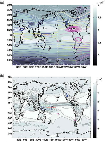
Figure 3. Contour maps of 36-year (432-month) averages of full atmosphere geopotential height (Z) and evaporation minus precipitation (EP) for the period 1979–2014: (a) full atmosphere Z (kg/m), and (b) full atmosphere EP (mm/d). Labels are defined in the text. Source: http://www.cgd.ucar.edu/cas/catalog/newbudgets/index.html#ERBEFs – files ERAI.Z.1979–2014.nc, ERAI.EP.1979–2014.nc.

As indicated above and in the Appendix (A1 and A3), geopotential heights (Z) of the full atmosphere drop significantly over major high-altitude land masses at middle latitudes, and those indentations are routinely indicative of enhanced atmospheric moisture. Figure 2(b) accordingly extends the exploration to streams originating from such regions, and includes three streams from the Southern Rocky Mountains, one Utah stream from further north in the same mountain range, and one from a Himalayan watershed. The graphic result, which is limited largely to the satellite era, suggests that significant lagged correlations between those streams and the WEP features of Figure 2(a) can be identified.

As suggested in the Appendix, the advent of full atmosphere coverage, with the satellite era starting in 1979, was essential for the current approach. Given this satellite era limitation and the lagged correlation between the solar signature and the atmospheric parameters introduced in Figure 2(a), it appears possible to apply a cross-regression moving average (CRMA) approach for their prediction. Moreover, given the lagged correlation between those atmospheric parameters and the streamflow signatures introduced in Figure 2(b), it also appears possible to apply a CRMA approach for streamflow prediction. In essence, these two correlative pairings represent the potential for an accurate, two-step CRMA analysis connecting solar cycles to streamflow records. There may be further potential in forecasting directly between a solar precursor and a stream, should the stream express a similar autocorrelation function (acf) curve to that of the solar time series.

Approach and methodology

Based on the conceptual development and supporting information of the previous section, a new set of targeted teleconnected hydrospheric correlations was explored with the goal of improved CRMA-based streamflow forecasting. Candidate watersheds included those associated with the Himalayas in south-central Asia, the Andes in South America, and the Southern Rocky Mountains in western North America. Moreover, the results of the CRMA approach to these streams may be compared to equivalent forecasts by other contemporary methods, including autocorrelation approaches.

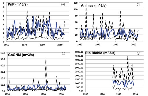
Figure 2(b) is an overlay of several of the candidate time series: one hydrograph from the Ganges River, draining the southern Himalayas, three from the Southern Rockies (Pecos, Animas, and Gila), and one from the Central Rockies (Lake Fork, LFRUT¹¹ ). Many of the featured time series have longer records than shown, but are truncated to fit the span of Figure 2(a), which starts roughly 70 years ago in 1950. The shortest complete record is that for the Ganges station. The current forecasting approach focuses on a satellite-era time span and is explored in more detail within the Discussion section. Salient details of each stream, including location, drainage areas and elevations of the highest catchment zones, are featured in Table 3. Locations of each gage are mapped in Figure 3(a) and (b). Notably, the streamlines shown in Figure 3(a) are explored in greater detail within Appendix A1, but are not of specific interest to the current exercise. The Ganges EF4 gage is identified by “C” in Figure 3(a). As profiled in Bharati and Jayakody (2004), the Ganges drains a major watershed extending to the Himalayas in the north, which are easily identified by the corresponding extreme indentation in the geopotential height contours. The Lake Fork, Utah, streamflow gage (Fig. 3(a), D) is shown as the open (blue) circle in western North America, and the three southern Rocky Mountain gages are represented by the solid (blue) dots adjacent to the “B” label. Within that domain, the Animas is the northernmost gage, the Pecos is the central gage to the east and the Gila gage is at the southern end of the cluster. Most state boundaries of the Western USA (other than Montana) are included in Figure 3(a) for additional context. As explored in the Appendix, the positions of the selected streamflow gages with respect to the geopotential height depressions (which can also be identified in Fig. 3(a)) are expected to influence the performance of this forecasting approach.

Table 3. Candidate stream gages.

River, State, Country	Gage ID	Longitude	Latitude	Drainage area (km^2)	Elevation of highest edge of catchment (km a.m.s.l.)	Years of continuous records available
Ganges River, Kanpur, India	EF4 Bithur	80.27472	26.61639	86 950	7.5	36
Pecos River, NM, USA	PnP	254.31730	35.70835	490	4.0	86
Animas River, NM, USA	Animas	251.79825	36.72250	3 522	4.2	85
Gila River, NM, USA	GnG	251.46261	33.06150	4 828	2.7	88
Lake Fork River, UT, USA	LFUT	249.474	40.60667	202	3.9	52
Rio Biobío, Chile	RBB	287.5	–36.8305	24 263	3.5	27

For this initial study, long-term records had been sought from pristine streams reaching into upper catchments without diversion. However, the EF4 gage near the Himalayas is understood to be influenced to some extent by anthropogenic activities, including extensive upstream reservoir management along with significant irrigation. Also, the records used from the EF4 gage have a very limited available time line and only express an annual resolution.

It is understood that many streams express seasonal variations that can sometimes be significant. However, in this study, the forecasts of primary interest address time spans of greater than one year. Although the longer time span permits a discount of seasonal effects, they remain of interest, especially for future improvements to the featured methodology. Towards that end, the three final chart sets in Figures A4–A6 superimpose the average July (coarse dotted line) and January (fine dotted line) variations over the annual averages (solid line) for the primary featured time series. Figure A4 covers these ranges for the well-known ocean drivers AMO, PDO, and ENSO. Figure A5 addresses the ranges for some of the additional indexes profiled in this study, namely the TWWP, the OLR, and the LEDIV. Finally, Figure A6 summarizes these seasonal variations for the four streams of primary interest. These charts reinforce that seasonal effects can be most pronounced for streams, whether in the northern or southern hemispheres.

Figure 4. Autocorrelation functions (acf) for 5-year trailing averages (5yta) of the SSN, TWWP, and selected streamflow observation time series.

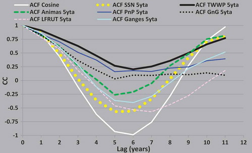
Figure 5. Autocorrelation functions (acf) and cross-correlation functions (ccf) for annual averages of the SSN, TWWP, and selected streamflow observation time series.

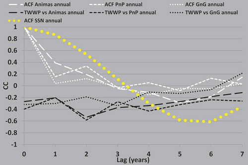
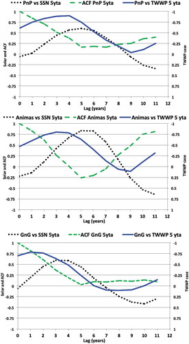
Figure 6. Cross-correlation and autocorrelation functions for 5-year trailing averages (5yta) of selected time series related to URGW watersheds: (a) PnP, (b) Animas, and (c) GnG.

Regardless of the seasonal variations (which are notable) and given their overall fit to the desired criteria, the remaining exercises are limited to the three representative streamflow records from the southern Rocky Mountains. The first featured site is the Pecos River near Pecos, New Mexico, gage (PnP), which captures water from a catchment that reaches over 4 km in elevation and resides within the noted geopotential indentation at a middle latitude (approx. 37°N). This gage lies largely upstream of any significant human operations such as reservoirs and irrigation. The Pecos River drains ultimately to the Gulf of Mexico within the greater Atlantic Ocean. The second featured site is the Animas River gage near Farmington, New Mexico. The Animas gage shares nearly all of the same characteristics as the Pecos. However, its flow rates are roughly 5–10 times higher than those of the Pecos, and it drains ultimately to the Upper Colorado River, which discharges into the Pacific Ocean.

The third site, the Gila River near Gila (GnG), New Mexico, was chosen for several reasons, but primarily due to its marginal qualities with respect to the candidate criteria. The Gila’s uppermost catchments are relatively high, but not quite as high as those of the Pecos and the Animas. As a tributary to the Lower Colorado River, the Gila also drains ultimately to the Pacific Ocean. While the other two catchments reach above 4 km in elevation, the upper elevation of the crest of the Gila watershed is only slightly below 3 km. Moreover, the Gila watershed is further to the south of the middle latitude target (at approx. 33°N). As a more marginal candidate, the Gila can be useful to ascertain some of the bounds for the optimal connections for greatest forecasting performance.

An exploration of the autocorrelations for each time series is helpful in targeting some of the most useful moving averages and lags for the forecasting exercises. Figure 4 outlines a series of autocorrelation functions (acf) associated with the SSN and TWWP indexes along with the selected streams. The maximum lag considered was 11 years, specifically because that is the primary period of the SSN index. Figure 4 has many notable features, for example, the acfs of the Sun and the Animas River are congruent for the most part. Moreover, to a greater or lesser extent, each acf shows a cyclostationary behavior, with a dip to low or negative autocorrelations near the 5-year lag followed by a return to higher and more positive ACFs near the 11-year lag. For context, the acf for the cosine function has been included (the white curve in Fig. 4), highlighting that the more regular the cycle for any given time series, the more it can resemble a sinusoid. Figure 4 also suggests that, as streams more remote to the Animas are queried, their acfs trend further away from that ideal cosine curve.

In further advancing the ARMA exercises, it is also understood that autocorrelations are sometimes developed when other candidate precursors cannot be determined. Time series studies, such as those by Machiwal and Jha (2010, Fig. 4) seek then to identify and filter out high AC anomalies even as far out as 9 years of lag. The purpose of eliminating autocorrelative persistence from time series studies also often relates to a goal of achieving pdfs that fit classical forms. From those pdfs, the familiar mean and variance moments can then be derived and used in the conventional forecasting approach.

The current exercise, as noted earlier, adopts a CRMA and ARMA comparative approach. It assumes that the persistence (even if intermittent) of a high autocorrelation pattern is correspondingly suggestive of underlying precursors, otherwise cyclic behavior, or both. The series of profiles of acfs and ccfs explored in Figures 5 and 6 might aid in a better understanding of the relative ranges of correlative values of this potential. Figure 5 focuses on annual average acfs and ccfs between selected SRM streams and the candidate precursors, while Figure 6 focuses on a 5-year trailing average (5yta).

Notably in Figure 6(b), the cross-correlation between the Sun and the Animas gauge exceeds 0.75 for a lag of 5–6 years. That points to the potential for additional forecast applications which can apply greater lags in fewer steps than those considered currently in this study. Accordingly, a related exercise that directly projects Animas flows from the solar cycle precursor is included towards the end of this section. Figure 6 also indicates that the highest multi-year correlations for all streams and precursor sets were found for a 3- to 4-year lag between the PnP and the TWWP. The GnG curves (Figs. 5 and 6) indicate generally lower correlations for each precursor, with a greater overall similarity to the Pecos (PnP) than to the Animas.

Unlike the acfs and ccfs of Figures 4 and 6, the annual average counterparts of Figure 5, display behaviors that resemble the hydrology acfs in Figure 4 of Machiwal and Jha (2010). Moreover, the “bump” in correlation at 2 years’ lag appears to be universal to this population and could be largely attributable to autocorrelation. This is noted for the best raw correlation for any moving average condition.

The steps explored in this exercise of the CRMA approach, utilizing both solar and WEP parameters, are geared towards the development of more accurate and longer-span hydrological forecasting for selected streams of the Rocky Mountain region. There are several limitations to consider. First, the improvements that are documented are not intended to verify the conceptual model described in Appendix A3. Rather, the conceptual model only provides a starting basis and structure for the exercises. Second, as the conceptual treatment outlines, there are likely geographical limitations to the applicability of this method. Following the conceptual model, the perceived limits of applicability in North America may follow roughly along the channel within the ridge in geopotential height of the full atmosphere (Z). This north–south channel overlies the Rocky Mountains footprint, as indicated by the related troughs in Figures A1(a) and (b). Third, as Figure 2(a) suggests, the actual correlations between the SSN and the WEP parameters are not linear over the entire time period shown. In the perspective of the 5-year trailing average applied, the SSN and WEP fluctuations appear to be synchronous until approximately 1990, upon which an increasing lag is indicated. Naturally that is suggestive of an inhomogeneity in the time series.

However, although a growing lag between the solar forcing series and the WEP signatures is evident, that is not observed so far between a WEP signature and a mountain stream. For this study only two CRMA simulations invoke the solar precursor and the remainder explore the CRMAs for the more homogeneous series. Best practices will require continual re-evaluation, updating, and likely adjustments to remain effective and relevant over the decades to come. In the current evaluation, the two-step approach benefits from parsimony of coefficients as well as the potential to address the apparent inhomogeneity.

In this context, the proposed method is subsequently shown to produce a promising yet variable degree of improvement across the study region. The first step of the process developed and applied the lagged correlations between each stream gage and the satellite-era TWWP for two different planning horizons: the first case produces a 5yta streamflow forecast with a lead time of 3 years into the future, and the second predicts an annual streamflow result 2 years into the future. These two CRMA conditions were decided upon in a manner consistent with the explorations of optimal cross- and autocorrelations at various lags, which are profiled in Figures 4–6. As part of this initial step, those correlations are applied to the customary linear regression solution as:

(1) $y=Ax+B$(1)

where x is the independent variable (TWWP for the first regression step), y is the dependent variable (streamflow for the first regression step), A is the dimensionless regression coefficient calculated from a linear fit of a scatter plot between historical values of y and x, and B is the intercept (the value of y when x is equal to zero).

Accordingly, Pearson correlation coefficients are calculated between the TWWP and each stream for the two lags and moving averages considered. Table 4 summarizes the coefficients, the correlations, and their statistical significance scores. In this analysis any additional autocorrelation impacts are simply inferred from Figures 4–6, which have been included to provide a complementary and clear comparison of the TWWP-based correlations to the calculated correlations when the traditional AC method is employed, as well as to a direct SSN precursor case. Figures 5 and 6 and Table 4 also document that for all streams, for the two lags and moving averages of primary focus, the TWWP correlations are largely the highest. Moreover the TWWP correlations generally show the highest significance scores.

Table 4. Linear regression coefficients and outcomes for the featured cases. 1yta, 5yta: 1-year trailing average, 5-year trailing average. AC: autocorrelation. PnP, Animas, and GnG are the streams as defined in text.

Regression case, x–y	A	B	Number of pairs, N	Pearson’s CC	R^2	Highest calculated percentile of significance
SSN–TWWP 5yta, 2-year lag	0.0157	4.0111	33	–0.7533	0.5675	99%
SSN–OLR 5yta, 2-year lag	na	na	38	–0.6366	0.4053	99%
TWWP–PnP 1yta, 2-year lag	13.596	137.51	36	–0.5833	0.3402	99%
AC–PnP 1yta, 2-year lag	0.3293	69.56	36	0.3356	0.1126	95%
TWWP–PnP 5yta, 3-year lag	–21.609	156	30	–0.8912	0.7941	99%
AC–PnP 5yta, 3-year lag	0.5688	42.173	30	0.5125	0.2626	99%
TWWP–Animas 1yta, 2-year lag	–85.803	1041.5	35	–0.5349	0.2861	99%
AC–Animas 1yta, 2-year lag	0.1835	675.27	30	0.1923	0.037	<90%
TWWP–Animas 5yta, 3-year lag	–143.76	1167.8	30	–0.799	0.6383	99%
AC–Animas 5yta, 3-year lag	0.2888	572.84	30	0.2652	0.0703	<90%
TWWP–GnG 1yta, 2-year lag	–11.507	212.08	36	–0.1876	0.0352	<90%
AC–GnG 1yta, 2-year lag	0.1197	161.79	36	0.1217	0.0148	<90%
TWWP–GnG 5yta, 3-year lag	–31.646	258.39	30	–0.6389	0.4082	99%
AC–GnG 5yta, 3-year lag	0.3568	113.74	30	0.3633	0.1320	95%
SSN–Animas 5yta, 5 yr lag	2.7029	543.22	33	0.8269	0.68376	99%

na: not applicable.

For completeness, Table 4 also includes a final set of correlations between the OLR and SSN time series. Just as for the SSN to TWWP connection, the OLR to SSN correlation is also found to be high and statistically significant at the 99th percentile. However, the OLR is not used further in this analysis, as the correlations are not as high as were determined for the TWWP.

Returning to the streamflow time series, the consistently high performance for the TWWP correlation results adds confidence that the approach can provide an improvement over a conventional forecast. The forecasts are developed by applying Equation (1) and utilizing the appropriate A and B linear regression coefficients from Table 4 for the given lags to the independent TWWP time series, as well as to the AC variation. The application of both ARMA and CRMA approaches for the three stream gages to two time-scale sets – a 3-year forecast of a 5-year trailing average and a 2-year forecast of an annual average – leads initially to 12 calculated time series for subsequent skill evaluation. An additional step to advance the forecast span is motivated for two of the streams by the correlations indicated between the TWWP and solar cycles in Figure 2(a). Moreover, solar cycles themselves are routinely forecast in advance by 1 year, as documented for example at the WDC-SILSO site. Accordingly, the second step entails first obtaining a record of 5yta SSN values to the current time, and then adding the projected SSN values for the subsequent year. Next, the Pearson correlation coefficient is calculated between the SSN record and the TWWP for a 2-year lag. The resulting regression coefficients are calculated and used to forecast the 5yta TWWP for 3 additional years into the future.

These projected TWWP values were then utilized, again through the regression relations of Equation (1) and Table 4, to predict the 5yta streamflows of the Pecos and Animas rivers for an additional 3 years into the future. For those specific cases, therefore, streamflows were quantitatively predicted for a total of 6 years beyond the year 2016. The results of this final step are appended to those from the previous step for the two relevant cases.

As described for Figure 6(b), a high lagged correlation also exists directly between the Animas and the SSN series without the need for a TWWP intermediate factor. It is therefore of interest to also explore the skill of this more parsimonious example. Accordingly, a single realization of the CRMA forecast of 5yta flows within the Animas River based on a 5-year lag following solar cycle changes is included for a 13th skill evaluation.

Results

Performance results are featured for specific cases from application of the widely used cross-regression and autoregression moving average (CRMA and ARMA) approaches towards time series predictive analyses. In the context of the three SRM stream records featured in this study, Figures 7 and 8 accordingly highlight overlays of predictions in comparison to observations for the 12-month (annual, 1yta) and the 60-month (5yta) cases. As identified in Figures 7 and 8, the solid lines represent observations and all other time series represent the various forecasts.

Figure 7. Comparison of predicted to observed values for the three SRM streamflow gages for the 12-month or annual average (1yta) cases. Blue: Animas; green: Gila (GnG); and black: Pecos (PnP). Vertical red line: boundary at the end of June 2016 between the training period and the test period. [For color refer to the online version.]

Figure 8. Comparison of predicted to observed values for the three SRM streamflow gages for the 60-month average (5yta) cases. Blue: Animas; green: Gila (GnG); and black: Pecos (PnP). Vertical red line: boundary at the end of 2015 between the training period and the test period. Dotted vertical red line: beginning of a solar-based forecast extension propagated through the TWWP series. [For color refer to the online version.]

This study also features a related and more parsimonious forecast of a 5yta Animas forecast based on an equivalent SSN series lead by 5 years. The vertical solid red lines in Figures 7 and 8 signify the boundaries between the training and test periods, while the dotted vertical red line (Fig. 8) signifies the beginning of a solar-based forecast extension propagated through the TWWP series for some of the 5yta cases.

Figures 7 and 8, along with the sum of additional correlation and regression performance metrics featured in Table 5, document that the TWWP tends to produce the most accurate forecasts, particularly for the two streams located well within the main target domain identified. Skill performances are routinely quantified through the common root mean squared error (RMSE). However a simple CC fit metric between observations and model results is also included in these results. Finally a greater sensitivity in the quantitative comparison of results between the forecast and observation populations was desired. Accordingly, two goodness-of-fit (GOF) measures were adapted from common significance and hypothesis testing resources: the well-known chi-squared (χ²) and Kolmogorov-Smirnov (K-S) tests.

Table 5. Performance results. RMSE: root mean square error; K-S: Kolmogorov-Smirnov. See Table 4 caption for explanation of other abbreviations.

Forecast case	RMSE	ρ value of χ^2 test	χ^2 test significance at ρ < 0.1*	ρ value of K-S test	Autocorrelation of residuals
SSN 2-year lead forecast of TWWP 5yta	0.71	2.94E-03	N	0.6	0.581
TWWP 2-year lead forecast of PnP 1yta	1.0455	3.25E-07	N	0.361	0.012
AC 2-year lead forecast of PnP 1yta	1.1726	9.36E-10	N	0.0222	na
TWWP 3-year lead forecast of PnP 5yta	0.3182	0.106	Y	0.893	0.054
AC 3-year lead forecast of PnP 5yta	0.6022	0.014	N	0.361	na
TWWP 2-year lead forecast of Animas 1yta	6.7083	0.0003	N	0.361	−0.013
AC 2-year lead forecast of Animas 1yta	7.7917	1.73E-22	N	0.043	na
TWWP 3-year lead forecast of Animas 5yta	3.1279	0.438	Y	0.893	−0.123
AC 3-year lead forecast of Animas 5yta	5.0446	2.91E-14	N	0.043	na
TWWP 2-year lead forecast of GnG 1yta	2.8875	8.49E-39	N	0.022	0.072
AC 2-year lead forecast of GnG 1yta	2.9178	3.51E-19	N	0.011	na
TWWP 3-year lead forecast of GnG 5yta	1.1188	0.1797	Y	0.531	0.089
AC 3-year lead forecast of GnG 5yta	1.3550	0.0013	N	0.231	na
SSN 5 yr lead forecast of Animas 5yta	3.3822	0.591	Y	0.983	na

*N: not significant; Y: significant; na: not applicable.

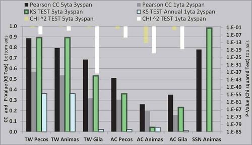
Results of the GOF and related CC performance estimates for the 13 regression calculations are summarized in Figure 9. In this summary of three simple quantitative measures, the TWWP forecasts for the most part outperform the conventional AC forecasts for the same cases over many degrees of freedom. Notably, Figure 9 also confirms a strong CC and GOF skill for the direct SSN-Animas forecast compared to the observed record.

Table 5 not only complements Figure 9 via a list of the key variables and outcomes for each ARMA and CRMA exercise, but also includes items not captured in Figure 9, including the RMSE values, and a measure of the autocorrelation of the residuals. In comparing among these exercises, some of the individual features of the GOF implementations remain evident. For example, the χ² goodness-of-fit calculations rely on a number of idealizations, including that the time series can be well represented by a normal or gamma distribution and that each bin in the developed histograms is sufficiently populated. Those idealizations are not perfectly captured for this comparison study. The χ² has utility nonetheless because it captures more than the first moment of a distribution, which is all that the initial performance index parameter, the RMSE can capture.

Figure 9. Comparison of Pearson correlations and goodness-of-fit indexes Kolmogorov-Smirnov (K-S) and chi squared (χ²) for three streams in relation to precursors.

The K-S method does not rely on an assumption of normality, yet typically K-S GOF methods work best as the populations approach continuous distributions. Given the relatively short time frames utilized (~33 years), both GOF methods are being applied in somewhat marginal territory. The final estimates are simply provided as a summation of performance measures, which collectively can help to determine the usefulness of the proposed forecasting method. The potential interference from autocorrelations is addressed this time by calculation of the AC of the residual for given cases. These are also included in the final column of Table 5. With one exception, the values do not support a prevalent autocorrelation component.

Discussion

As noted, the purpose of this study was to explore and evaluate a new methodology for the improvement of streamflow forecasting. The method was targeted at regions that satisfied criteria related to global positioning and altitude with respect to Hadley and Walker circulation limbs and possible teleconnections to an atmospheric moisture source. That source is consistent with a conceptual model which posits that solar irradiance fluctuations lead to corresponding fluctuations of moisture, heat, and wind in the region of the planet with the greatest concentration of atmospheric moisture, namely the so-called “hot tower” overlying the WEP. The purpose of this study has not been to prove or disprove such a solar-based notion. However, given the previous literature, along with the superior regression-based forecast performance of the featured method, such conceptual questions appear to merit further discussion.

One question of particular interest relates to the two distinct temporal behaviors of the solar and “hot tower” patterns depicted in Figure 2(a). Clearly, the SSN, the trade winds, and the OLR patterns first exhibit a stable and synchronous pattern for many years, followed by a marked downward trend, with a growing separation between the three signatures that extends to this day, even as the oscillations continue. One possible explanation might be related to the observation that the SSNs achieved historic maximums towards the middle of the 20th century and then began a descent, as described in the Introduction section.

Perhaps over the maximum solar phases, energy inputs were sufficient to significantly raise associated Hadley, Walker, and zonal circulation rates. At such presumed higher circulation rates, shorter transit times might have produced the relatively synchronous responses of the hot tower to solar conditions. If that were the case, then it might follow that lower energy solar inputs would lead to slower and less energetic Hadley and Walker circulation rates, with an accordant decrease in the footprint of the hot tower. This might explain the expanding lag between the solar signal and the hot tower signals over the second half of the time series. Suggestions of increases in Hadley circulation rates for moisture and heat transport due to greater climate temperature forcings are in fact common within modern climate science references (Hoyt and Schatten 1997 Chapter 6, Otto-Bleisner and Clement 2005).

Also, a similar transition in solar–climate patterns from synchrony to a phase change is partially documented from over a century ago. As noted by Hoyt and Schatten (1997), for the mid to late 19th century, synchronous solar–climate patterns were independently described by Koppen (1914) and Meldrum (1885), the former for temperature and the latter for frequencies of Indian Ocean cyclones. Relatively high sunspot numbers were also persistent over that period, but were followed by the Gleissberg Minimum, a multi-decadal period of relatively low sunspot numbers that extended into the early 20th century. Accordingly, it can be said that the arrival of the Gleissberg Minimum was accompanied by the loss of synchronous correlations to those climate indexes. Moreover, the current drop in sunspot numbers associated with Solar Cycle 24 may be more than a brief and minor event. According to researchers such as Ahluwalia (2012), the contemporary plunge in sunspot numbers is suggestive of the advent of another grand minimum, such as the Dalton or Gleissberg minima.

An additional question regards the wider applicability of this investigation, given that the geographical study area of impacted streams is so limited. The Southern Rocky Mountain study area does indeed have a small footprint, but it is still an important one, partly because it resides along a continental divide. It is notable for example that one stream of the study, the Pecos River, flows east to the Atlantic Ocean, while a second stream, the Animas, flows west to the Pacific Ocean. Accordingly, the impacts of these upper watersheds have at least some consequences extending for hundreds of miles (km) downstream.

Furthermore, with regard to the relatively low flow rates of the targeted streams, the economics are not inconsequential. A general contemporary price in the Western USA for irrigation water can reach over US$1000 per acre foot (over US$100 per hectare meter) (Vekshin 2014), whereas some estimates of water prices in areas along the Front Range of the Rocky Mountains are documented to reach over $30 000 per acre foot ($3700 per hectare meter) (Center of Colorado Water Conservancy District¹² ). Given the significant differences between the RMSE values for the forecast methods shown, significant cost savings appear to be achievable if the TWWP approach were adopted and proved to be successful.

The current study area also covers a smaller footprint along a lower latitudinal zone than the previously described Canadian river studies of Prokoph et al. (2012) and Fu et al. (2012). Perhaps those differences can explain why SRM streams display more notable coherence in relation to SSNs than those within Canada to the north. For example, Section 4.3.2 of the Fu et al. (2012) study indicates that some of the statistically significant correlations are positive and others are negative. Moreover, as Figure 1 of that study illustrates, connections appear to rise and fall somewhat periodically with increasing distance from the Pacific (Atlantic).

Nonetheless, incorporation of lagged correlation studies along the lines of the current study may add value to future forecasting applications for some streams in the Canadian study areas. Those perhaps might be most successful in their Rocky Mountain watersheds, because the Prokoph et al. (2012) study noted that those regions displayed the greatest connections to SSNs for an 11-year cycle. Moreover, in addressing some streamflow records within the Rocky Mountains, the Prokoph study concluded that “… major floods are more likely to occur during sunspot cycles with relatively low sunspot numbers after the last maximum.” Remarkably, the same came be said of SRM streams in this investigation. For example, a review of Figure 2 of this investigation demonstrates that for the 5yta condition the high and low extrema of the SRM streams in Figure 2(b) align fairly well to the concurrent solar cycle low and high extrema in Figure 2(a). Clearly, in this study the connection is attributed to a set of lagged correlations to solar maxima, whereas the Prokoph et al. (2012) investigation did not explore the alternative of a lagged effect.

The apparent correspondence between Canadian Rocky Mountain streams and those of the current study within the Southern Rocky Mountains may therefore reinforce the conceptual model that serves as the foundation of this study. As previously described and as featured particularly in the Appendix (Figs A1(a) and (b)), the indentations in geopotential height along a narrow channel that aligns with the Rocky Mountain cordillera throughout North America pass through both the relevant high solar correlation portions of the Prokoph et al. (2012) study to the north and this study to the south.

The Himalaya watersheds also fit the desired latitudinal and geopotential profiles that are believed to lead to improved forecasting using the featured methodology. These signatures are indicated in Figures 3(a) and (b) and A1(a) and (b). Also, as demonstrated in Figures 2(b) and 4, the time series history and the ACF pattern of a gage on the Ganges River display encouraging similarities to those of the SRM streams.

Significant challenges are nonetheless expected to emerge with regard to any desired extensions of this technique to wider geographical areas. Perhaps the practical and geographical limits have already been outlined in this single study. Yet, given similar solar connections to other regions of the atmosphere and even other watersheds, there are reasons to be optimistic. As noted previously, past researchers have indicated that solar cycle signatures in the upper troposphere appear to diminish rapidly with decreasing altitude (Labitzke and Van Loon 1995). Accordingly, with continuing improvements in instrumentation, and increasing epistemic knowledge of this new set of connections, it may be possible in the future to identify fainter and/or less obvious signatures, and thereby successfully apply a form of the featured technique to additional watersheds.

Other improvements appear possible or at least plausible. One opportunity might be in the development of various extensions of the two moving averages and lag sets featured here, even down to the resolution of a monthly scale with a lead time of several years. For example, the Pearson correlation coefficient between the solar monthly series for 1991–2011 and the TWWP monthly series for 1994–2014 is calculated as −0.47. Given the count of 252 monthly data pairs, this is statistically significant at the 99th percentile.

There may also be significantly different residence times of the moisture and heat circulating via Hadley cells and related patterns (see Appendix A1) through the Northern and Southern Hemispheres. Those differing rates may lead to two different average arrival times back to the Inter-Tropical Convergence Zone (ITCZ) resulting from the solar irradiance pulses that roughly uniformly bathe the Earth, associated with sunspot cycling over climatological scales. As described in Gray et al. (2010), the Southern Hemisphere circulation is expected to be much more rapid than that of the Northern Hemisphere.

Such an explanation might be further supported by the previous observation concerning the Parana stream in the Southern Hemisphere. That South American stream is reported to express a high correlation to SSNs, yet with little or no temporal lag (Mauas et al. 2008). South America presents a much smaller continental footprint within the Southern Hemisphere in comparison to regions of the Northern Hemisphere. Along with the reduced interference to atmospheric circulation associated with such domains as the Southern Annular Mode (Limpasuvan and Hartmann 1999), this would be consistent with a model in which the Southern Hemisphere “solar pulse” signature within the atmosphere always returns to the WEP region before its Northern Hemisphere equivalent.

The mouth of the Rio Biobío (also termed the Rio Bio Bio) on the Chilean coast of South America, within the town of Desembocadura (Fig. 3, H), was examined to explore this question within a modest framework. A supporting representation of the seasonal and annual climatologies of the Rio Biobío for its somewhat limited time series from 1982 to 2008 is presented in the Appendix (Fig. A6). As is the case for the Gila stream (also in Fig. A6), the seasonal summer drought is a relatively stationary feature of this stream. Moreover, the normalized curves of Figure 10 display an apparent 5-year average consistency of this stream record with its Southern Hemisphere neighbor the Southern Pacific Convergence Zone (SPCZ), as captured in part by the SOI at its Tahiti monitoring point.

Figure 10. Comparison of normalized 5-year trailing averages (5yta) for two ENSO parameters and the Rio Biobío. Sources for Rio Biobío: Government of Chile Water Directorate, 2004, CUENCA DEL RIO BIO BIO, Cade-Idepe Engineering Consultants.

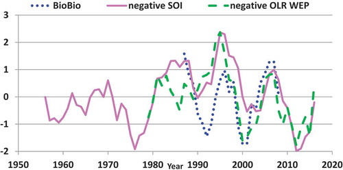
Unlike the Parana River within the same continent, the Rio Biobío is a river that extends from a middle latitude watershed into the westerly winds at the coast, and its uppermost catchments also reach above the 3.5 km elevation mark. According to the conceptual model featured here, these aspects make the river a logical candidate site for further testing. Moreover, the previously mentioned concept of a more rapid Southern Hemisphere circulation is reinforced by the Rio Biobío time series record, since there is no longer a persistent lag between the WEP OLR signature and the stream record. Unfortunately, as also suggested by information within the Parana paper (Mauas et al. 2008), this reduces the available lag to be used for regression-oriented forecasting in that hemisphere down to the lag between the SSN and the SOI, OLR, or other associated climate parameter.

Additional studies, including papers by Diaz et al. (1992, Fig. 5) and Keith (1995, Figs 6 and 7), further support the overall dominance of the Southern Hemisphere with regard to zonal circulation rates within the atmosphere and the ocean. Yet, even with a qualitative understanding of differential circulation rates between the two hemispheres, it would remain important to quantify how rapidly and to what level of coherence, zonal-dominated moisture and heat circulation patterns eventually migrate towards the ITCZ, which is a primary feature of Hadley circulation theory.

More contemporary studies of Hadley-driven zonal and meridional circulations have typically been geared towards other questions than comprehensive comparisons of hemispheric residence times. Those questions have focused primarily on the scale of meridional expansions and contractions of the Hadley cell, the meridional migrations of the ITCZ about the equator, and/or the meridional and regional variations in the zonal winds of the middle latitudes (Bowman and Cohen 1997, Lorenz and Hartmann 2001, Shaw and Voigt 2016, Nguyen et al. 2018). Some first order consistency can nonetheless be found, including Bowman and Cohen’s inference that “the time required to mix tropospheric air between the Northern and Southern Hemisphere extratropics is on the order of 1 year.”

Some papers that directly tackle questions of the variation of residence times of moisture and heat between the Northern Hemisphere and the Southern Hemisphere appear to avoid higher latitude zones and also place significant reliance upon GCMs and related and general thermodynamic “aquaplanet” simulations (Shaw and Voigt 2016). Other papers, including Aggarwal et al. (2012), have developed atmospheric moisture residence time estimates at points across the globe based on stable isotope analyses for ¹⁸O. That paper surveyed numerous studies and described a strong linear signal between the enrichment of ¹⁸O and the estimated residence time of the moisture of precipitation, in a manner consistent with the global meteoric water line. However, the work was limited to the troposphere and screened out residence time estimates greater than 100 days. The screening may have been predicated on expectations of residence times within that lower atmospheric layer. The recent work on meridional overturning by Linz et al. (2017) potentially offers additional insights, including a representation that residence times of upper atmospheric parcels can range from 0 to 8 years at the poles and from 0 to 2 years along the ITCZ. It may be notable that the two studies provide contrasting estimates of residence times, and so the topic will remain of research interest. In the perspective of this study, it is believed that the major gyres will play dominant roles for the near and long term of any circulatory residence time conceptualization.

Gyres, overturning, solar forcing, and many other variables continue to pose challenges to circulatory residence time mapping. This study has simply contributed to demonstrations of the potential for improved accuracy in multi-year predictions of annual and multi-annual average streamflows, regardless of whether or not the adopted precursors were truly causal or simply coincidental. This is a valid exploration regardless of causality because of the potential practical benefits, so long as practitioners remain mindful of the open-ended questions such as those profiled here.

Summary and conclusions

Considerations of past research regarding solar cycles, Hadley and Walker circulation patterns, and streamflow characteristics of several mid-latitude, high-altitude watersheds have pointed to the potential for improved multi-annual to sub-decadal forecasting of streamflows in targeted locations. Such conditions appear to apply to Northern Hemisphere watersheds of the Himalayas as well as the Southern Rocky Mountains of the Western USA. Conditions also appear favorable in some Southern Hemisphere watersheds of the Andes, with the caveat that forecast spans are expected to be shorter in potential. The initial examples studied do not yet define any limit throughout the American Cordillera.

In the development of these conclusions, a set of correlations and linear regressions were explored for key sequential features based on previous published research and currently available solar (SSN), trade wind (TWWP), outgoing longwave radiation (OLR), geopotential height (Z), divergence of latent heat (LEDIV), and other indexes. Equivalent exercises were applied towards potential connections of some of those parameters to streamflow datasets for candidate streams of the Rocky Mountains. A two-stage regression-based forecasting approach was then applied to exploit some of the highest lagged correlations that were identified. The forecasts were compared to forecasts for the same streamflow datasets via a conventional autocorrelation technique.

The training forecasts based on the new CRMA applications were generally the most accurate of all featured methods, for the series considered under a 5-year trailing average. Through a sequence of solar and trade wind regression exercises, forecasts for this set were advanced as far as 6 years into the future. The forecasts under the new method were also found to be more accurate than the conventional method under an annual average with a 2-year lead forecast approach, although the fidelity of all results was diminished in comparison to the 5-year average set of forecasts. An additional but limited investigation demonstrated high-fidelity 5-year trailing average forecasts for the Animas River based directly on solar cycles taking place 5 years in advance.

The success of the proposed methodology is expected to apply to other regions meeting the target criteria, including the Ganges River in India and the Rio Biobío in Chile. Subsequent exploration of monthly correlations between the TWWP and sunspot cycles suggests that, for appropriate locations, advances of hydroclimate forecasting accuracy with monthly resolution yet multi-annual lead times may also be possible through the new technique.

Disclosure statement

No potential conflict of interest was reported by the author.

Notes

¹ http://www.cpc.ncep.noaa.gov/products/analysis_monitoring/lanina/enso_evolution-status-fcsts-web.pdf.

² http://www.cpc.ncep.noaa.gov/products/analysis_monitoring/ensostuff/ensoyears.shtml.

³ http://www.sidc.be/silso/; http://www.esrl.noaa.gov/psd/data/timeseries/AMO/; http://research.jisao.washington.edu/pdo/PDO.latest; https://www.ncdc.noaa.gov/teleconnections/enso/indicators/SOI/.

⁴ publications.iwmi.org/pdf/HO43412.pdf.

⁵ USGS 08378500 Pecos River near Pecos, NM; USGS 09364500, Animas River at Farmington, NM; and USGS 09430500 Gila River near Gila, NM, available from: https://waterdata.usgs.gov.

⁶ http://www.cgd.ucar.edu/cas/catalog/newbudgets/index.html#.

⁷ http://www.aoml.noaa.gov/hrd/hurdat/comparison_table.html.

⁸ http://www.cgd.ucar.edu/cas/catalog/newbudgets/index.html#ERBEFs – file ‘ERAI.LEDIV.1979–2014.nc.

⁹ http://www.cpc.ncep.noaa.gov/data/indices/wpac850.

¹⁰ https://www.ncdc.noaa-gov/teleconnections/enso/indicators/olr/.

¹¹ USGS 09289500 Lake Fork River AB Moon Lake, Nr Mountain Home, UT, available from: https://waterdata.usgs.gov.

¹² http://centerofcoloradowater.com/?page_id=2 [Accessed 22 Nov 2017].

¹³ http://www.cpc.ncep.noaa.gov/products/analysis_monitoring/lanina/enso_evolution-status-fcsts-web.pdf.

¹⁴ http://www.cpc.ncep.noaa.gov/data/indices/wpac850.

Appendix

The topics covered in sub-appendices A1–A3 serve to document the reproducible connections between solar cycles, atmospheric circulation, and streamflow time series, which serve as the conceptual basis for an alternate CRMA-based forecasting approach in the body of the paper.

A1 Global circulation principles and the quasigeostrophic approximation

It is well known that circulations of moisture and gases at any scale can often be approximately quantified with respect to potential energy and momentum states. The Navier-Stokes formulations bridge these potential states to the regional conditions in space and time. Moreover, equations of state, such as the hydrostatic equation and its cousin the hypsometric equation, provide powerful expressions that often accurately define the linear relationship between geopotential height, temperature, and pressure in a full atmosphere approximation.

In addition to diabatic processes and the movements of sensible heat, the manifold state changes possible for atmospheric moisture ensure that the capture, escape, and circulation of atmospheric heat are significantly influenced by the latent energy component. This includes the heat that is adiabatically removed from the surrounding atmosphere to evaporate and sublimate water and that is adiabatically returned to the atmosphere upon condensation of water vapor into clouds. The Clausius-Clapeyron equation, which is an exponential function of temperature differentials in particular, is often widely and reliably used to estimate the energy fluxes of latent heat from the atmosphere above large bodies of water.

The Hadley circulation defines a related meridional–global pattern of atmospheric transport. In this mapping, tropospheric air and moisture ascend from the tropics towards the stratosphere and then transport pole-ward, reaching middle to upper latitudes. Those limbs of the Hadley circulation are balanced by widescale subsidence into the westerly flow patterns of the lower atmosphere. The relative transport features of the Hadley circulation are complemented by additional momentum and heat signatures, which include the angular momentums of the subtropical gyres of the ocean and the atmosphere. Tropical and subtropical gyres can exert a dominant impact in their respective regions, as suggested by focused studies (Reid 1997, Kuhlbrodt et al. 2007, Groth et al. 2017). Additional investigations, such as those by Rhines and Young (1982), explore the significant momentum, dimensions, profiles, and solute and energy transports within paired major atmospheric and ocean gyres, while other authors, including Zhang and Chen (2008) and Qui and Chen (2012), describe in equivalent scope, but independently, the interwoven masses of the atmospheric warm pool (AWP) and ocean parcels. Notably, the AWP is attributed as having the greatest concentration of atmospheric moisture across the planet.

Researchers apply much contemporary focus on a subset of overall Hadley circulation known as the Brewer-Dobson (BD) meridional overturning circulation. These patterns have been explored in part to address mass and energy transport across the stratosphere–mesosphere boundary. The estimated maximum BD stratospheric overturning rate of nearly 10¹⁰ kg/s is notable (Linz et al. 2017). The entire mass of the Earth’s atmospheric moisture has been estimated to be approximately 1.3 × 10¹⁶ kg on average (Freeze and Cherry 1979, Trenberth and Smith. 2005). Residence times of moisture remain uncertain in regard to many characterizations. Moisture not entrained within gyres has been estimated to circulate zonally through the atmosphere within 9 days on a globally averaged basis (NOAA 2017¹³). This leads to an equivalent zonal moisture circulation rate of approximately 10¹⁰ kg/s.

Finally, the Walker circulation signifies a largely tropical coupling between lower atmospheric flows and upper atmosphere patterns between the Indian Ocean footprint and equivalent latitudes within the Pacific Ocean (Diaz and Bradley 2005). The extensive body of Hadley and Walker circulation literature (including the papers within Diaz and Bradley 2005) does not appear to highlight the role of atmospheric gyres. However, this conceptual model allows for the possibility that, given their broad footprints and persistence, the great tropical to subtropical gyres contribute to the seamless transitions from Walker circulation attributes to westerly zonal flows of the middle latitudes. For both the atmosphere and the underlying oceans, these gyres spin clockwise in the Northern Hemisphere and counter-clockwise in the Southern Hemisphere. The Discussion section of this paper explores residence times further in the context of the forecast results.

A significant departure of this conceptual model from conventional circulation literature is the consistent application of quasigeostrophic (QG) mapping over the entire planet. As a widely used forecasting and diagnostic tool, the QG approach synthesizes Coriolis-driven flow with hypsometric principles. The QG implementation is notable for many aspects, including its intrinsic simplification of the full atmosphere into a single layer, although that is typically limited to synoptic scales of approximately 1000 km.

Figure 3(a) and (b) within the main text introduces the current approach to mapping a planetary-scaled QG atmosphere as captured by a 36-year (432-month) average contour plot of geopotential height (Z) and evaporation minus precipitation (EP) for the full atmosphere, along with a distribution of equilibrium streamlines. The Z contour is a widely used variable, but typically applies for a range of elevations. Obviously, in this QG approach, the definition of Z is restricted to a measure of the specific weight of any defined full atmospheric parcel. The darkest values of contour bands therefore define the thinnest regions of the full atmosphere and the lightest shades define the thickest regions.

The equilibrium streamlines in Figure 3(a) facilitate further discussion of the gyres and overall full atmosphere circulation concepts. All streamline origins are designated by a white star. The blue stream lines originate along a constant longitude (7°E) near the left side of the charts. The magenta streamlines originate along a constant longitude (79°W) closer to the right side of each figure. A set of yellow streamlines originate along the 150°W longitudinal meridian, passing through E and G. Two final sets of white streamlines address polar and subpolar regions via origins along the 76°N latitude and the 89°S latitude. Streamline origin points are equally spaced 10° in the meridional direction and 20° in the zonal direction.

Figure 3(a) and (b) reinforces that the planetary scale QG implementation can reasonably represent many aspects of conventional meteorology. For example, the convergence of westerly streamlines displayed over North America is in alignment both geographically and conceptually to the well-known jet stream at that latitude span. Moreover, the meridional undulation of these jets can be reasonably compared for any given month to the associated and well-known polar vortexes. A similar correspondence applies to the equivalents in the Southern Hemisphere.

Figure 3(a) and (b) can also be used to identify other important atmospheric features. For example, the great concentration of EP mapped at the Western Equatorial Pacific coincides with the AWP, and includes several notable limbs, including one that extends towards Tahiti (Fig. 3(a), G). Tahiti is also a pivotal location for the calculation of the SOI. This high atmospheric moisture limb is known as the Southern Pacific Convergence Zone (SPCZ) (Kiladis et al. 1989).

As previously indicated, this QG contour and streamline mapping allows identification of the major gyres. They are captured by Figure 3(a) in part by the maximum Z light shaded ovals and also defined in part by related streamlines. In these representations, gyres show distinctive yet variable patterns. Streamlines that originate near or within a gyre commonly develop a path primarily limited to revolutions within the gyre boundary. Some gyre-trapped streamlines escape into the mid-latitude Westerlies. Also, some mid-latitude streamlines are trapped by gyres even as the main middle latitude masses of air proceed eastward, as expected via the widely recognized Coriolis effect.

Finally and notably, within the region defined by the ITCZ from approximately 10°S to 10°N, the streamlines show the well-known pattern of equatorial easterly winds. The ITCZ corresponds to a high concentration of atmospheric moisture via the EP coverage. The well-known pattern is also described as the “Equatorial Trough” due to the lower pressures associated with greater relative moisture (Houze 2003). This trough is featured below in more detail. Naturally, this is an average regime and, as later figures (Figs A1 and A2) suggest, there is significant variability from one monthly average to the next.

Because of the circulatory characteristics of the major gyres, the convergence and divergence of moisture across the boundaries of the ITCZ may not be as uniformly distributed as conventionally described. For example, the Western Hemisphere Warm Pool (WHWP) (Wang and Enfield 2001) appears to be roughly comparable with the AWP, since it is intimately associated with the two Atlantic and/or East Equatorial Pacific gyres. As noted by those authors, the net climatological effect of the circulation complex associated with the WHWP is lateral divergence from the Equatorial Trough at those longitudes towards the middle latitudes. The QG streamlines of Figure 3(a) support the Wang and Enfield (2001) observations with an apparently complementary impact of net convergence to the west of that WHWP domain. This pattern appears to be roughly mirrored in both Northern and Southern hemispheres.

A2 Contemporary studies of connections of global circulation to solar cycles

The topics surveyed here indicate that the multimodal circulation patterns of dry air, moisture, and heat (both latent and sensible) remain challenging to monitor, analyze, and predict. Moreover, the state changes of water associated with these regimes must be quantified to some level of fidelity in identifying aspects of solar forcing that impact those circulations. This may be considered a challenging prospect if only because contemporary correlations between the Sun and surface climate have not been widely or frequently reported (Gray et al. 2010). Some papers, such as Svensmark et al. (2009), have indirectly addressed this topic with respect to galactic cosmic rays and atmospheric moisture nucleation, but they appear to remain controversial and largely unverified. For example, as discussed in Gray et al. (2010), even if moisture patterns were found to correlate with cosmic rays, they would also be found to correlate with solar irradiance, and therefore uniqueness of causality would require further verification.

In any case, a limited set of additional connections between solar cycles and the troposphere and stratosphere over the Arctic and across North America have been quantitatively demonstrated in works such as Labitzke and Van Loon (1995), Van Loon and Shea (2000), Soon (2005), Meehl and Arblaster (2009), and Scaife et al. (2013). In particular, Labitzke and Van Loon (1995) identified a similar decadal oscillation signature to that of the solar cycle, and also proved correlations as high as 0.7 for selected temporal subsets of the 30-hPa geopotential height above North America and over the North Pacific Ocean (Fig. 3(a) and (b), E). Lateral variations of the correlations between solar cycles and the atmosphere have also been explored by some of the previous references, as well as in Hood and Soukharev (2012), who found notable connections between sea level pressure and SSNs in the northern Pacific, as well as additional broad areal patterns of statistically significant similarities.

Some of the prior solar atmospheric correlation studies explored concepts of a “top-down” and a “bottom-up” pattern of solar forcing upon the Earth’s atmosphere, such as Lockwood et al. (2010). However, to date there is no consensus regarding how climatological solar forcings propagate through the atmosphere or hydrosphere in any direction, whether vertical, meridional, or zonal. Labitzke and Van Loon (1995) provided examples of observations where the solar correlations diminish with decreasing elevation within the troposphere. Gray et al. (2010) also noted that the Earth’s exosphere from 500 to 1000 km elevation shows a clear 11-year solar cycle signature, but added that there is little evidence to suggest a propagation of that signature down to the surface. Finally, as mentioned, Lockwood et al. (2010) explored a top-down mechanism for the propagation of solar forcing towards decadal changes in tropospheric moisture. These descriptions were made in the context of an emerging understanding of atmospheric circulation patterns and radiant heat transfer, which continues to develop. As noted previously, a full atmosphere quasigeostrophic (QG) simplification is applied in this conceptual model. Through this simplification, the question of the propagation of the solar signature is reduced from a three-dimensional and/or purely vertical issue to a largely lateral one.

A3 Atmospheric moisture, geopotential indentations, and potential connections to solar cycles

Although the QG approximation is employed in this conceptual model, it remains important to note that most of the atmosphere’s water can be found within the troposphere. The troposphere extends from the Earth’s surface to the tropopause, which represents a temperature inflection and a transition to the lower stratosphere. Over the planetary scale, the tropopause consistently reaches its highest elevations (nearly 16 km) along the margins of the ITCZ. That height diminishes by several kilometers with increasing proximity to either pole. Within the ITCZ footprint, the tropopause typically attains its highest elevation above the Western Equatorial Pacific Ocean (5°S–5°N and typically 135°E–170°W), referred to herein as the WEP footprint.

This prominence has been identified by past researchers, including Malkus and Riehl (1964), Hartten and Gutzler (1998), and Houze (2003), the first having developed the concept of the “hot tower”. Not surprisingly, this zone also occupies the same general footprint as the noted AWP, which was defined, for example, by Zhang and Chen (2008) and mentioned above (Appendix A1), and encompasses the greatest concentration of atmospheric moisture across the planet. The same general boundaries also apply to the Ocean Rain Pool and the Oceanic Wet Pool, as identified by Wang and Enfield (2001) and Chen et al. (2004). Understandably, the footprint was an important focus of the Tropical Ocean–Global Atmosphere (TOGA) Coupled Ocean Atmosphere Response Experiment (COARE), which was executed through the collaboration of over 120 people from 20 nations in 1993 (Godfrey et al. 1998).

Some specific connections between solar cycles and the troposphere have been identified to date. The investigations of Van Loon and Shea (2000), among others, have indicated that “… the troposphere at stations near the ITCZ is warmed more by the release of latent heat at the solar maxima than in the minima.” Other researchers, such as Tourpali et al. (2005), have stated that a tropospheric modulation of the Arctic Oscillation (AO) extends into the stratosphere during years of high solar activity. Some of these studies accordingly support a related and perhaps obvious conclusion that an increase in solar forcing over annual time frames leads to an increase in upper tropospheric moisture over the ITCZ footprint.

The troposphere is also influenced by the underlying land surface. General patterns of tropospheric distortion by orographic effects are widely known and have been described by, e.g., Jacob (1999). These elevated areas are believed to exhibit enhanced hydrological responses to any tropospheric signal pattern for several reasons. First, high-elevation watershed catchments in temperate latitudes reach above the more turbulent and less predictable Planetary Boundary Layer (PBL) and extend accordingly into more rapid and laminar and less dense flows. For example, Hsu and Wallace (1985) pointed out such patterns for the Himalayas of Central Asia and the Rocky Mountains of western North America. As also suggested previously, in comparison to the tropics and subtropics, the tropopause is relatively lower in elevation over those temperate latitudes. Accordingly, the high-altitude catchments are much closer to the potential interception of teleconnected mid-latitude Hadley circulation moisture than any other continental regions.

From these perspectives, a useful teleconnection simplification is sought through the identification of regions of “source” atmospheric moisture concentrations within the ITCZ that may be particularly sensitive to solar cycles, in conjunction with the identification of “receptor” continental regions that accordingly would be impacted via circulation. In this context, the AWP is relevant as a potential moisture source location. Furthermore, Figure 3(a) enables the potential identification of candidate orographically influenced moisture receptors, through the geopotential height, Z, isocontours for the full atmosphere. The map verifies that the Z levels drop significantly across major high-altitude land masses in middle latitudes, including the Rocky Mountains of North America.

Figure A1(a) and (b) provides complementary and somewhat more literal representations of the planetary scaled geopotential height, Z. First it is noted that the gyres can be identified in Figure A1 as corresponding mounds emerging from the two zonal ridges that rim the equator to the north and south. For example, the north subtropical gyre (Fig. 3, F) consistently overlies the zone of highest geopotential height on the planet for this average coverage and for many subsets. Accordingly, the gyres can be seen to coincide with the largest mounds of the full atmosphere found across the planet. It is also relevant in context that the two panels of Figure A1, one mapping the average January condition (Fig. A1(a)) and the other mapping the average July condition (Fig. A1(b)), clearly show a solar impact. However, in this case the dramatic shifts of the Z parameter simply result from the changes in solar insolation over the course of each orbit of a tilted Earth around the Sun.

Of greater importance to this conceptual model is the observation in Figure A1 for both cases of the aforementioned Equatorial Trough in Z, logically along the equator, which naturally corresponds directly to the band of concentrated equatorial moisture seen in Figure 3(b). The dynamic relations of atmospheric moisture to geopotential height can be further understood in light of the conceptual illustrations in Figure A2(a) and examples of supporting meridional data profiles in Figure A2(b). As the WEP footprint is associated with high vertical wind velocities resulting from hot tower convection, it is understood that horizontal velocities in that domain within the lower troposphere are relatively diminished. This is supported by many sources, including an ENSO-related data coverage set of lateral trade winds maintained by the National Oceanic and Atmospheric Administration (NOAA) National Weather Service (NWS) Climate Prediction Center (CPC). In particular, the coverage for winds at 850 mb across the same WEP footprint is available for the period of satellite coverage.¹⁴ For brevity, and because no acronym is provided by the source, this coverage is termed herein as the TWWP (Trade Winds West Pacific) and it is implied that this is with respect to the lower troposphere layer at that pressure level. As also conveyed by the 5-year moving average coverages in Figure 2(a) of the main text, the TWWP annual time series shares much in common with other related parameters over the WEP footprint. For example, it is closely associated with the well-known outgoing longwave radiation (OLR) resource.

The OLR time series covers a period from 1974 to the present. It is defined as a longwave radiation signature at the top of atmosphere (TOA) over approximately the same TWWP footprint. This OLR footprint location is identified by the (red) horizontal line segment along the equator in Figure 3. The OLR is also a component of the ENSO index. As again suggested by Figure 2(a), the apparent connection of the OLR and many related parameters, including the SOI, the TWWP and the LEDIV, to the SSN oscillations appears to be strong. It can therefore be argued that the OLR and the TWWP directly register a solar impact on Hadley-circulated atmospheric moisture in the area of the AWP, which, as mentioned, has the Earth’s greatest concentration of atmospheric moisture.

Figure A2(b) provides documentation of the changes in Z and EP for a cross-section overlapping the WEP footprint, which is largely consistent with that concept. Examination of Figure A2(a) shows that this section crosses the Equatorial Trough, an equatorial band of consistently high moisture within the ITCZ. As the two adjacent annual average curve sets in Figure A2(a) indicate, the geopotential height surface appears to vertically migrate up or down over time in the fashion of a piston, whereas the EP parameter includes a lateral component to its migrations. Finally, the rises and dips in the EP are transformed to associated dips and rises of the Z profile. This is consistent with the knowledge that the vapor pressure of water is lower than that of dry air.

Although this observation might partially weigh on recent studies which indicate that ENSO connections to solar signals are inconclusive or at least intermittent (Roy and Haigh 2012), the OLR signature is also notable because of its significant relation to cloud formation over its footprint. Figure A2(a) illustrates that, as more cloud formation occurs, a greater amount of longwave radiation from the underlying Earth surface is blocked, and thus the OLR expression at the TOA diminishes. Conversely, as less cloud formation occurs, more longwave radiation reaches outer space past the TOA. According to this model, the response via both featured variables over the WEP footprint is one in which decreases and increases in the solar irradiance (as represented by SSNs) can be followed by decreases and increases in equatorial convective cloud-forming activity.

It is understood that EP patterns may show some consistency with latent heat patterns, through the Clausius-Clapeyron relationship, and in the context of circulation. As mentioned, the latent heat of condensation, LEDIV, was extracted from the same ERAI satellite records for the WEP footprint. The LEDIV is an independent record of convective activity as it reflects the heat released into the atmosphere from the condensation of water (included as the dotted blue line in Figure 2(a)); it is notably consistent with the other two WEP signatures.

Figure A3(a) shows that the correspondence between the LEDIV and OLR signatures is apparently strong even at a monthly resolution. The complementary images of Figure A3(b) delineate additional time series and areal coverages of the LEDIV from other locations within the same ERAI dataset. These locations include the Labitzke and Van Loon Pacific site (Fig. 3, E) and a location in the West Pacific associated with a major gyre (Fig. 3, F). Figure 3 may be consistent with the idea that the phase shifts between each record are related to whether or not each location is primarily within a gyre footprint. However, more work would be beneficial to extend or challenge the concept. The remaining expressions of LEDIV in Figure A3(b) extend the mapping of the LEDIV parameter across the main teleconnections of this study area. These maps suggest, among other things, that the geostrophic full atmosphere energy of latent heat can routinely exceed ±200 W/m². This compares favorably with the average TSI values on a monthly basis, and further reinforces the importance of atmospheric moisture in regard to solar connections from both a dynamic and an energy balance perspective, given that the average solar forcing upon the Earth’s surface is generally indicated to average 239 W/m² (Gray et al. 2010).

Much of this discussion has revolved around the Equatorial Trough, which, as is the case for any pressure trough, indicates a concentration of moisture in the atmosphere. That trough is evident in the surface plots of Figure A1(a) and (b), which also indicate another trough associated with the Rocky Mountains for both the boreal winter and summer. This persistent and seasonally influenced, relatively narrow channel itself rests upon a higher ridge of geopotential height, which can be termed the “Rocky Mountain Hanging Trough” and is a candidate for the teleconnected moisture reception previously discussed. In fact, it can be said that the entire American Cordillera, including both the Andes and the Rocky Mountains, are known to display this hanging trough.

Figure A1. January and July 1979 full atmosphere geopotential height (Z, kg/m) surfaces, oblique quasi-3D view: (a) January 1979, and (b) July 1979.

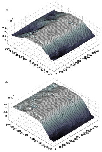
Figure A2. Comparisons of solar forcing conceptualization to limited observations: (a) conceptualization of the Equatorial Trough, and (b) profiles through the Western Equatorial Pacific of the Equatorial Trough.

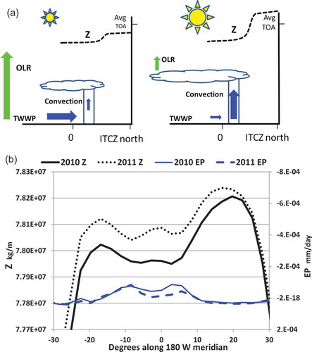
Figure A3. Charts and maps featuring divergence of latent heat (LEDIV) over the WEP region and other locations across the Pacific Ocean. (a) Monthly values for the OLR index and LEDIV over the WEP region. (b1) Time series of 5yta of LEDIV for selected Pacific locations. Maps of magnitude of 5yta LEDIV for the full atmosphere, across North America and much of the Pacific: (b2) 1980–1985 and (b3) 2009–2014.

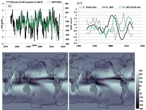
Figure A4. (a) AMO index, (b) PDO index, and (c) ENSO index. Solid line: annual; coarse dotted line: July; fine dotted line: January.

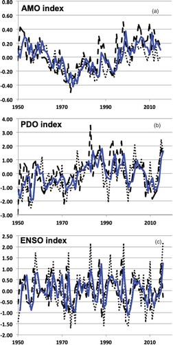
Figure A5. (a) TWWP index, (b) OLR sample index, and (c) LEDIV sample index. Solid line: annual; coarse dotted line: July; fine dotted line: January.

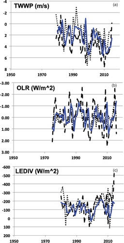
Figure A6. (a) PnP index; (b) Animas index; (c) GnG index; and (d) Rio Biobío index. Solid line: annual; coarse dotted line: July; fine dotted line: January.

References

- Aggarwal, P.K., et al., 2012. Stable isotopes in global precipitation: a unified interpretation based on atmospheric moisture residence time. Geophysical Research Letters, 39, L11705. doi:10.1029/2012GL051937
- Ahluwalia, H.S., 2012. Three-cycle quasi-periodicity in solar, geophysical, cosmic ray data and global climate change. Indian Journal of Radio & Space Physics, 41, 509–519.
- Bharati, L. and Jayakody, P. 2004. Hydrology of the Upper Ganga River. International Water Management Institute, publications.iwmi.org/pdf/HO43412.pdf.
- Bowman, K.P. and Cohen, P.J., 1997. Interhemispheric exchange by seasonal modulation of the Hadley circulation. Journal of the Atmospheric Sciences, 54 (16), 2045–2059. doi:10.1175/1520-0469(1997)054<2045
- Chen, G., et al., 2004. Observing the coupling effect between warm pool and “rain pool” in the Pacific Ocean. Remote Sensing of Environment, 91, 153–159. doi:10.1016/j.rse.2004.02.010
- Diaz, H.F. and Bradley, R.S., eds. 2005. The Hadley circulation: present, past and future. Dordrecht: Kluwer Academic Publishers.
- Diaz, H.F., Fu, C.B., and Quan, X.W., 1992. A comparison of surface geostrophic winds with COADS ship wind observations. In: Proceedings of the International COADS Workshop, January 13–15, 1992 Colorado, 131–141.
- Freeze, R.A. and Cherry, J.A., 1979. Groundwater. Englewood Cliffs, NJ: Prentice-Hall Inc.
- Fricker, T.E., Ferro, C.A.T., and Stephenson, D.B., 2013. Three recommendations for evaluating climate predictions. Meteorological Applications, 20, 246–255. doi:10.1002/met.1409
- Fu, C., James, A.L., and Wachowiak, M., 2012. Analyzing the combined influence of solar activity and El Niño on streamflow across southern Canada. Water Resources Research, 48, W05507. doi:10.1029/2011WR011507
- Godfrey, J.S., et al., 1998. Coupled ocean-atmosphere response experiment (COARE): an interim report. Journal of Geophysical Research, 103 (C7), 14395–14450. doi:10.1029/97JC03120
- Goldenberg, S.B., et al., 2001. The recent increase in atlantic hurricane activity: causes and implications. Science, 293. doi:10.1126/science.1060040
- Gray, L.J., et al., 2010. Solar influences on climate. Reviews of Geophysics, 48. doi:10.1029/2009RG000282
- Groth, A., et al., 2017. Interannual variability in the North Atlantic Ocean’s temperature field and its association with the wind stress forcing. Journal of Climate, 30, 2655–2678. doi:10.1175/JCLI-D-16-0370.1
- Hartten, L.M. and Gutzler, D.S., 1998. Estimates of large-scale divergence in the lower troposphere over the western equatorial pacific. Journal of Geophysical Research: Atmospheres, 103, 25895–25904. doi:10.1029/98JD02171
- Hood, L.L. and Soukharev, B.E., 2012. The lower-stratospheric response to 11-yr solar forcing: coupling to the troposphere-ocean response. Journal of the Atmospheric Sciences, 69, 1841–1864. doi:10.1175/JAS-D-11-086.1
- Houze, R.A., 2003. From hot towers to TRMM: Joanne Simpson and advances in tropical convection research. Meteorological Monographs, 29, 37. doi:10.1175/0065-9401(2003)029<0037:CFHTTT>2.0.CO;2
- Hoyt, D.V. and Schatten, K.H., 1997. The role of the sun in climate change. New York, NY: Oxford University Press.
- Hsu, H.H. and Wallace, J.M., 1985. Vertical structure of wintertime teleconnection patterns. Journal of the Atmospheric Sciences, 42, 1693–1710. doi:10.1175/1520-0469(1985)042<1693:VSOWTP>2.0.CO;2
- Jacob, D.J., 1999. Introduction to atmospheric chemistry. Princeton, NJ: Princeton University Press.
- Kalra, A., et al., 2013. Using large-scale climatic patterns for improving long lead time streamflow forecasts for Gunnison and San Juan River Basins. Hydrological Processes, 27, 1543–1559. doi:10.1002/hyp.9236
- Keith, D.W., 1995. Meridional energy transport: uncertainty in zonal means. A: Dynamic Meteorology and Oceanography, 47 (1), 30–44. doi:10.3402/tellusa.v47i1.11492
- Kiladis, G.N., von Storch, H., and Van Loon, H., 1989. Origin of the South Pacific convergence zone. Journal of Climate, 2 (10), 1185–1189. doi:10.1175/1520-0442(1989)002<1185:OOTSPC>2.0.CO;2
- Koppen, W., 1914. Lufttemperaturen, Sonnenflecke und Vulkanausbruche. Meteorlogische Zeitung, 31, 305–328.
- Kuhlbrodt, T., et al., 2007. On the driving processes of the Atlantic meridional overturning circulation. Reviews of Geophysics, 45. doi:10.1029/2004RG000166
- Labitzke, K. and Van Loon, H., 1995. Connection between the troposphere and stratosphere on a decadal scale. Tellus A: Dynamic Meteorology and Oceanography, 47 (12), 275–286. doi:10.3402/tellusa.v47i2.11505
- Limpasuvan, V. and Hartmann, D., 1999. Eddies and the annular modes of climate variability. Geophysical Research Letters, 26, 3133–3136. doi:10.1029/1999GL010478
- Linz, M., et al., 2017. The strength of the meridional overturning circulation of the stratosphere. Nature Geoscience, 10, 663–667. doi:10.1038/ngeo3013
- Lockwood, M., et al., 2010. Top-down solar modulation of climate: evidence for centennial-scale change. Environmental Research Letters, 5 (3), 034008. doi:10.1088/1748-9326/5/3/034008
- Lorenz, D.J. and Hartmann, D.L., 2001. Eddy-Zonal flow feedback in the Southern Hemisphere. Journal of the Atmospheric Sciences, 58, 3312–3327. doi:10.1175/1520-0469(2001)058<3312:EZFFIT>2.0.CO;2
- Machiwal, D. and Jha, M.K., 2010. Comparative evaluation of statistical tests for time series analysis: application to hydrological time series. Hydrological Sciences Journal, 53 (2), 353–366. doi:10.1623/hysj.53.2.353
- Malkus, J.S. and Riehl, H., 1964. Cloud structure and distributions over the tropical pacific ocean. Tellus, 16, 275–287. doi:10.1111/tus.1964.16.issue-3
- Mauas, P.J.D., Flamenco, E., and Buccino, A.P., 2008. Solar forcing of the stream flow of a continental scale south American river. Physical Review Letters, 101, 1–4. doi:10.1103/PhysRevLett.101.168501
- Meehl, G.A. and Arblaster, J.M., 2009. A lagged warm event–like response to peaks in solar forcing in the Pacific Region. Journal of Climate, 22, 3647–3660. doi:10.1175/2009JCLI2619.1
- Meldrum, C. 1885. On a supposed periodicity of the cyclones of the Indian Ocean south of the equator. British Association Report, 925–926.
- Nguyen, H., et al., 2018. Variability of the extent of the Hadley circulation in the southern hemisphere: a regional perspective. Climate Dynamics, 50 (1–2), 129–142.
- Otto-Bleisner, B.L. and Clement, A., 2005. The sensitivity of the Hadley circulation to past and future forcings in two climate models. In: H.F. Diaz and R.S. Bradley, eds. The Hadley circulation: present, past and future. Netherlands: Kluwer Academic Publishers, Vol. 15, 437–464.
- Prokoph, A., Adamowski, J., and Adamowski, K., 2012. Influence of the 11 year solar cycle on annual streamflow maxima in southern Canada. Journal of Hydrology, 443, 55–62. doi:10.1016/j.jhydrol.2012.03.038
- Qui, B. and Chen, S., 2012. Multidecadal sea level and gyre circulation variability in the Northwestern Tropical Pacific Ocean. Journal of Physical Oceanography, 42, 193–206. doi:10.1175/JPO-D-11-061.1
- Reid, J.L., 1997. On the total geostrophic circulation of the pacific ocean: flow patterns, tracers, and transports. Progress in Oceanography, 39, 263–352. doi:10.1016/S0079-6611(97)00012-8
- Rhines, P.B. and Young, W.R., 1982. A theory of wind-driven circulation. I. Mid-ocean gyres. Journal of Marine Research, 40 (Supplement), 559–596.
- Roy, I. and Haigh, J.D., 2012. Solar cycle signals in the Pacific and the issue of timings. Journal of the Atmospheric Sciences, 69, 1446–1451. doi:10.1175/JAS-D-11-0277.1
- Scaife, A.A., et al., 2013. A mechanism for lagged North Atlantic climate response to solar variability. Geophysical Research Letters, 40, 434–439. doi:10.1002/grl.50099
- Schwabe, A.N., 1844. Sonnen-Beobachtungen im Jahre, 1843. Astronomische Nachrichten, 21, 234–235. doi:10.1002/(ISSN)1521-3994
- Shaw, T.A. and Voigt, A., 2016. What can moist thermodynamics tell us about circulation shifts in response to uniform warming? Geophysical Research Letters, 43, 4566–4575. doi:10.1002/2016GL068712
- Soon, W., 2005. Variable solar irradiance as a plausible agent for multidecadal variations in the Arctic-wide surface air temperature record of the past 130 years. Geophysical Research Letters, 32, 1–5. doi:10.1029/2005GL023429
- Svensmark, H., Bondo, T., and Svensmark, J., 2009. Cosmic ray decreases affect atmospheric aerosols and clouds. Geophysical Research Letters, 36, 1–4. doi:10.1029/2009GL038429
- Tourpali, K., et al., 2005. Solar cycle modulation of the arctic oscillation in a chemistry-climate model. Geophysical Research Letters, 32, 1–4. doi:10.1029/2005GL023509
- Trenberth, K.E. and Smith., L., 2005. The mass of the atmosphere: a constraint on global analyses. Journal of Climate, 18, 864–875. doi:10.1175/JCLI-3299.1
- Van Loon, H. and Shea, D.J., 2000. The global 11-year solar signal in July-August. Geophysical Research Letters, 27, 2965–2968. doi:10.1029/2000GL003764
- Vekshin, A. 2014. California-water-prices-soar-for-farmers-as-drought-grows. Available from: http://www.bloomberg.com/news/articles/2014-07-24/BloombergNews7-24-2014 [Accessed 10 Aug 2017].
- Wang, C. and Enfield, D.B., 2001. The tropical Western Hemisphere warm pool. Geophysical Research Letters, 28 (8), 1635–1638. doi:10.1029/2000GL011763
- Wang, S.Y., et al., 2010. Coherence between the Great Salt Lake level and the Pacific Quasi-Decadal Oscillation. Journal of Climate, 23, 2161–2177. doi:10.1175/2009JCLI2979.1
- Wei, W.S., 2006. Time series analysis, univariate and multivariate methods. Boston: Pearson Addison Wesley.
- Zeng, X., Wang, D., and Wu, J., 2015. Evaluating the three methods of goodness of fit test for frequency analysis. Journal of Risk Analysis and Crisis Response, 5 (3), 178–187. doi:10.2991/jrarc.2015.5.3.5
- Zhang, C. and Chen, G., 2008. The atmospheric wet pool: definition and comparison with the oceanic warm pool. Chinese Journal of Oceanology and Limnology, 26, 440–449. doi:10.1007/s00343-008-0440-6