Simulation of spatially-distributed copper pollution in a large river basin using the ECOMAG-HM model

ABSTRACT

The semi-distributed physically-based model ECOMAG-HM was developed to simulate cycling of heavy metals in large river basins: on the surface, and in soil, groundwater and river water. The model was applied to study the spatial distribution and temporal dynamics of copper concentrations in watercourses of the Nizhnekamskoe Reservoir watershed in Russia. This watershed is characterized by high background concentrations of heavy metals due to wide occurrence of ore deposits and considerable concentrations of ore-parent elements in rocks. The model was found to adequately reproduce the spatial variation of the mean annual copper concentrations at different monitoring points of the river network. The mean annual specific copper washoff, with the surface and subsurface components of river runoff, and the total copper washoff from the watershed into the river network were calculated and mapped. The contributions of natural and anthropogenic factors to river water pollution by copper were evaluated.

KEYWORDS:

• ECOMAG-HM model
• river basin
• runoff formation
• pollutants
• copper washoff
• mapping

Editor R. Woods Associate editor I. Battiato

1 Introduction

The microcomponents of surface water chemistry related to heavy metals (HMs) are involved in biochemical processes of vital activity in aquatic animals, and they can be limiting factors or, at higher concentrations, toxicants. Heavy metals are conservative pollutants, i.e. they do not decompose in natural water but could be consumed or transported. The major processes of self-purification of watersheds and water bodies from HM compounds are their removal from watersheds by surface and subsurface runoff, transport with river discharge, and settling with sediments into the bottom deposits (Linnik and Nabivanets 1986).

Usually, the HM concentrations in water bodies show considerable variability in space and time due to natural and anthropogenic factors. The soil-geological and climatic conditions in a watershed, along with the features of runoff genesis in different water regime phases, govern the dynamics of HM concentrations coming from diffuse sources. Additional inflow of HMs could be from point sources due to economic activities in the watershed (industrial and municipal wastewater). The anthropogenic pollution of water bodies by HMs is most noticeable in places where mining works and heavy industry are concentrated. When the open method of ore deposit extraction is applied, emission of HM and other pollutants in the atmosphere occurs due to intense dusting. All stages of the technological process of extraction and processing of minerals are accompanied by the formation of large volumes of wastewater. Pollutants accumulate in places of permanent wastewater releases from industrial enterprises and downstream in the bottom sediments of watercourses. Pollution of groundwater occurs in the areas of oil fields, near the storage of liquid and solid wastes from various industries, and in places of storage of solid wastes (landfills). The major pathways for metals to enter water bodies from anthropogenic sources are: polluted precipitation from the atmosphere onto the watershed surface, surface washoff, leaching from the subsurface, wastewater discharge, and inflow from polluted aquifers or bottom sediments.

According to Russian State statistical reports, the discharge rates of industrial wastewater and the amounts of pollutants they contain has dropped considerably in recent decades (Barenboim et al. 2013). Partly, this decrease was due to the closure of some industrial enterprises in the post-Perestroika period. Another reason was the implementation of measures at industrial enterprises for protection of water bodies: better water treatment facilities and water saving technologies which contributed to the reduced discharge of polluted wastewater to water bodies. However, this has not led to improvement of water quality in many water bodies, as could be expected. In our opinion, this is due to the absence of reliable knowledge about the contributions of natural and anthropogenic sources to the pollution of water bodies. The development of strategies to manage quality of water resources in river basins requires studying processes that influence river water quality, and quantitative assessment of pollutant inputs from sources that differ in genesis, and spatial and temporal characteristics. For studying the spatial distribution and temporal dynamics of HMs in river basins and forecasting changes in the hydrochemical regime resulting from water protection measures, considering also possible changes in climate, land use and economic activities, one needs a deterministic process-based mathematical model, which includes all these processes and their interrelations.

The development of methods for simulating pollution of river catchments by nutrients started in the 1960s, mostly due to the environmental pollution caused by the application of fertilizers in agriculture. In the beginning, these methods were based mainly on empirical relationships for calculating pollutant washouts from polluted areas using correlations with hydrological parameters (Bedient et al. 1980). The CREAMS model (Chemicals Runoff and Erosion from Agricultural Management Systems; CREAMS 1980) was one of the first conceptual field-scale models of water quality that included a description of processes. A review of many modifications of conceptual models describing water quality formation in areas with nonpoint spatial pollution can be found in Yang and Wang (2010), Gao and Li (2014), Harmel et al. (2014) and Krysanova et al. (2009).

Since the 2000s, spatially-distributed or semi-distributed models of pollutant washoff and river water quality have been used to solve problems of diffuse and point-source pollution. Small sub-catchments, or so-called hydrological response units (HRUs) within them, which are homogenous with respect to soil type, land use and elevation, are used as calculation units in such models. Among others, the Soil and Water Assessment Tool (SWAT) model is widely used for simulation of river discharge and pollution loads at different scales: from the continental scale (Abbaspour et al. 2015), through the regional scale (Santhi et al. 2008), to the scale of individual river catchments (Galvan et al. 2009, Zhang et al. 2013). The SWAT model may evaluate the effects of different management scenarios on watershed hydrological processes as well as on point and nonpoint source pollution. There are SWAT applications investigating heavy metal pollution as well (Galvan et al. 2009, Leebai et al. 2016).

Being especially successful, the semi-distributed models were used for the rivers of Germany in the implementation of the European Water Framework Directive for the evaluation of measures to reduce contaminant loads and improve ecological status of water bodies. For example, in Fuchs et al. (2017), the pathway-oriented conceptual model MoRE (Modelling of Regionalized Emissions) was used to simulate regionalized emissions of different pollutant sources with yearly temporal resolution for the strategic planning of specific measures to reduce the overall pollutant emissions into water bodies of Germany. A geographical information system (GIS)-based conceptual model METALPOL was validated using the measured heavy metal loads in the Elbe River basin (Vink and Peters 2003), and applied for analysis of scenarios, which indicated that the currently proposed measures are not stringent enough to achieve substantial reductions in heavy metal loads. It was shown that future management strategies should focus more on the reduction of emissions from diffuse sources, which contribute more than 70% of the total heavy metal emissions. A more detailed, process-oriented model, the Soil and Water Integrated Model (SWIM), was calibrated and validated against the observed water discharge and water quality data for gauges located in the Elbe River basin (Hess and Krysanova 2016). After that the model was applied to assess impacts of changes in climate and land use on the water regime and nutrient transport in the river network at the watershed scale.

In this study, the spatio-temporal dynamics of copper in a watershed is analysed using the semi-distributed, physically-based model ECOMAG-HM (ECOlogical Model for Applied Geophysics – Heavy Metals), which consists of two major blocks: hydrological and hydrochemical submodels. The hydrological model ECOMAG (Motovilov et al. 1999a, 1999b, Motovilov 2016a) has been tested successfully for many river basins in different physiographic zones at different spatial scales: from small catchments in Scandinavia (Motovilov et al. 1999b), with drainage areas of several square kilometres, to the great Volga and Lena rivers, with watershed areas exceeding one million square kilometres (Motovilov 2016b, 2017). The model was proved to be efficient for simulating both river discharge in different points of the river network and the dynamics of hydrological fields (soil moisture content, snow water equivalent and runoff) in large river basins. Since 2004, the ECOMAG model has been utilized in operational mode for the simulation of hydrological characteristics and water inflow into the Volga-Kama and Angara-Yenisey reservoir cascades in Russia (Gelfan and Motovilov 2009), among the largest reservoir cascades worldwide.

The hydrochemical submodel ECOMAG-HM was used to assess the contribution of the Pechenganikel’ Mining Company to anthropogenic river water pollution in the northwestern part of the Kola Peninsula (Motovilov 2013). For many years, the rivers in this region were among the most strongly polluted by heavy metals in Russia. The simulation results showed that, in the case of the plant’s operation being fully terminated, it would take about three decades for river waters to purify to the background level.

The focus of this study is the spatial and temporal dynamics of runoff and copper in the large watershed of the Nizhnekamskoe Reservoir (NKR). For several decades, copper compounds have been among the most widespread pollutants of surface water in this region due to the wide occurrence of ore deposits, with considerable concentrations of ore-parent elements in rocks, and intensive extraction and use of these natural resources. Another factor in favour of the choice of this study basin was the availability of detailed hydrochemical monitoring data (Fashchevskaya et al. 2018), as well as data on the spatial distribution of heavy metals in soils of the region (Yaparov 2005). The main purpose of the study was to quantify the contributions of direct anthropogenic (wastewater) and diffuse components to pollution of water bodies by copper, which is necessary for planning measures to reduce copper pollution in the watershed. The specific objectives of the study were to assess the ECOMAG-HM model potential for (a) simulation of the hydrological and hydrochemical regimes of river discharge and copper concentrations; (b) simulation of the spatial fields of runoff and copper washoff to the river network; (c) simulation of the pathways of copper washoff in a spatial mode; and (d) assessment of the contributions of diffuse and point anthropogenic sources to copper pollution in the NKR watershed.

2 Materials and methods

2.1 Semi-distributed hydrological model ECOMAG-HM

The hydrological submodel of ECOMAG-HM describes the processes of a land hydrological cycle, i.e. snow cover formation and snowmelt, freezing and thawing of soil, infiltration of rain and snowmelt water into soil, evaporation, dynamics of soil moisture content, as well as surface, subsurface and groundwater flows and river discharge. The equations, algorithms and testing results of the hydrological submodel are described in several papers (Motovilov et al. 1999a, 1999b, Motovilov 2016a, 2016b, 2017).

The hydrochemical submodel, aimed at the description of migration and transformation of conservative pollutants in catchments, accounts for processes of pollutant accumulation on land surfaces, dissolution by melt and rainwater, penetration of dissolved forms of pollutants into soil, and interactions with soil solution and soil solid phases (Motovilov 2013). Dissolution of pollutants, which fall from the atmosphere onto the land surface as dry deposition, is described as a linear function of the difference between the maximum possible and current concentrations in the surface flow. The rate of pollutant added from soil to surface flow is calculated as a linear function of the difference between their concentrations in soil and flowing water. The process of sorption–desorption of chemicals in soil is described by the linear Henry sorption isotherm relating the amount of a sorbed matter and its concentration in the solution. Complete and instantaneous solute mixing is assumed for each water storage under consideration.

The lateral diffusive inflows of dissolved pollutants to the river network by the surface, subsurface and groundwater flows depend on the intensity of hydrological processes. That is why hydrological variables determined in the hydrological submodel are used in the hydrochemical submodel. The transfer and transformation of pollutants in the river system are described taking into account the lateral diffusive inflow of pollutants, the load of pollutants from point sources to the river and exchange of pollutants between the river water and riverbed.

In the schematization of a river basin for modelling, its surface is divided by an irregular grid into elementary watersheds using GIS, taking into consideration relief and river network structure. The hydrological and hydrochemical processes in each elementary watershed are simulated at four levels (Fig. 1): on the surface, in the upper soil layer (horizon A), in the underlying deeper soil layer (Horizon B), and in the groundwater storage. In the cold season, snow-cover storage is also taken into account.

Figure 1. Structure of (a) the hydrological submodels and (b) the hydrochemical submodels of ECOMAG-HM.

The main equations of the ECOMAG–HM model are listed in the Appendix.

2.2 Study area

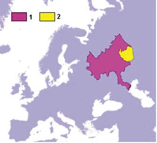
The watershed of the Nizhnekamskoe Reservoir is located on the Kama River, the largest tributary of the Volga River (Fig. 2). The NKR watershed occupies the area between the Nizhnekamskiy and Votkinskiy hydropower plants. Most of the NKR watershed is the basin of the Belaya River, the main river in the southern Urals. A considerable part of the watershed lies within the Republic of Bashkortostan (RB), with its capital Ufa city. The catchment of the NKR has an area of 186 000 km². About two-thirds of the watershed area, its western and central parts, is flat, whereas its eastern part belongs to the Ural Folded Mountain Area. The average height of the basin is 392 m a.s.l., and its highest elevation – Yaman-Tau Mountain – is 1654 m a.s.l. Forests account for about 50% of the territory, and the lake area is very small. The soils in the area (chernozem, sod-podzol and grey forest soil) have a high humus content and heavy texture. Well-drained mountain soils are widespread in the eastern part of the watershed.

Figure 2. Location of the Nizhnekamskoe Reservoir watershed (2) in the Volga River basin (1).

The location of the basin in the huge Eurasian continent, far from seas and oceans and close to the semi-deserts of Kazakhstan and Caspian Lowland, determines its continental climate. The Ural Mountains create conditions for the basin to be subject, on the one hand, to the effects of warm and wet water masses from the Atlantic, and, on the other hand, to the effects of the severe continental climate of Siberia. Therefore, one can see a variety of climate conditions here: from semi-arid steppe regions, with annual precipitation of 300–400 mm and mean annual air temperature of about 3°C, to wetter regions (northeastern and eastern mountain-forest areas), with annual precipitation exceeding 600 mm and mean annual air temperature lower than 1°C. The climate differences in the watershed area cause distinct latitudinal zonality of vegetation (steppe, forest-steppe and forest zones), additionally complicated by the vertical zonality in the Ural Mountains zone.

The intra-annual distribution of river runoff in the region characterizes the water regime as a typical snow-dominated one. The spring flood accounts for more than 60% of the annual runoff. The mean annual lateral water inflow to the NKR is 36.5 km³, of which 26.1 km³ are delivered by the Belaya River. The surface water bodies are the main sources of water supply to the economy and population of the region. However, water resources show considerable spatial and seasonal variability. The specific runoff in the central and western sub-regions, where the majority of the population reside, is three to five times lower than that in the eastern mountain sub-region. Due to that, water resources become deficient in some areas in dry years. That is why about 400 reservoirs and ponds with volumes above 100 000 m³ and many smaller ponds are in operation in the basin.

The rivers of the region are exposed to pollution by copper compounds to a large degree. In particular, the recurrence of copper concentrations in river water in the examined watershed rising above the maximum allowed concentration (MAC) for waters used for fisheries (0.001 mg L⁻¹) is 50% or more (Chernogayeva 2017). The main reason for that is a specific feature of the geological structure of the area, with wide occurrence of ore deposits and high concentrations of ore elements in rocks, resulting in higher background concentrations of metals in groundwater and surface water. More than 3000 deposits and manifestations of different types of raw materials have been discovered in RB territory (Bashkortostan 1996). The soils inherit the chemical composition of the soil-forming rocks. The metals in soils form stable complexes with humic substances and leave them very slowly: the period for soil copper content reduction by a half exceeds 1000 years (Maistrenko et al. 1996).

Additional sources of metals in soils and water bodies are economic activities in the region. In the eastern part of the region, these include mining plants; in its western and central parts, these are oil production and processing, chemical and petrochemical, metallurgical, mechanical engineering, and power generation plants, as well as storage facilities for production and consumption wastes. The industrial development of the region, which started more than 300 years ago, consisted mostly in exploitation of mineral deposits, and was carried out without any ecological limitations. In the late 18th century, copper-smelting plants were already in operation in the region, accounting for more than 50% of copper production in Russia at that time (Bashkortostan 1996). At present, the eastern part of the region (lowland Transuralia) contains large deposits of copper sulfide ore. The ore lies near the land surface and can be mined from open pits; these have been mined with variable intensity over a long time. In the open-pit mining of ore deposits, all process operations (the separation of rocks from the massif by drilling or explosions, their fragmentation, sorting, transportation to storage sites, and accumulation in dumps) are accompanied by intense amounts of dust and release of HM and other pollutants into the atmosphere. As they are washed out from the atmosphere, precipitating onto the soil and accumulating in its top layer, the metals create local technogenic anomalies in soils around the pollution sources. As a result, the concentration of copper in soils near industrial centres and mining regions can be more than one order of magnitude higher than the average mass fraction of copper in soils of the world (20 mg kg⁻¹) (Ezhegodnik 2011, Gosudarstvennyi 2005).

All stages of the extraction and processing of raw materials produce large amounts of wastewater. Wastewaters of mining plants are extracted along with useful minerals (open pit and mine drainage, drainage water), and form in the process of ore beneficiation (process tailings etc.), or result from precipitation (rainwater, snow melting in mine sites and under-dump water). Unfortunately, mining wastewater often reaches beyond the sanitary zone of the enterprise, it may not be localized, and may be discharged into surface water bodies without treatment. Pollutants enter the groundwater in areas of oil field development, near collectors of liquid wastes from plants of different industrial sectors, and at the storage sites of solid domestic wastes.

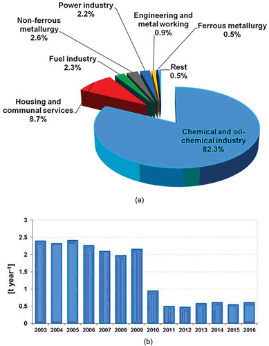
A considerable amount of HM enters water bodies with wastewaters from large populated localities, containing plants of various industrial sectors. Storm sewage forms from precipitation, which accumulates pollutants from the air and wash-settling aerosols, as well as street and road garbage, from urban territories and industrial sites. The composition of industrial wastewaters is governed by the chemical and petrochemical sector plants, mechanical engineering and metalworking, nonferrous and ferrous metallurgy, and the fuel industry (Fig. 3(a)). The result of this is high anthropogenic loads on water bodies, which influences their chemistry, including HM concentrations (Fig. 3(b)). A sharp drop in copper load after 2009 was due to a change in the calculation statistical method.

Figure 3. (a) Anthropogenic sources of copper in wastewater discharged to water bodies of the NKR basin and (b) dynamics of the total annual amount of copper in the discharged wastewater in 2003–2016 (Gosudarstvennyj 2005).

Thus, the major anthropogenic sources of copper (Cu) in the streams are “ancient” anthropogenically transformed mining landscapes, modern industrial plants for mining and processing mineral resources, large settlements, and their infrastructure facilities. The main paths of metal entering the streams from anthropogenic sources are as follows: precipitation from the atmosphere onto the water area and watershed surface, surface washout from the watershed, wastewater discharge, input from polluted aquifers or bottom sediments.

2.3 Model set-up for the NKR watershed

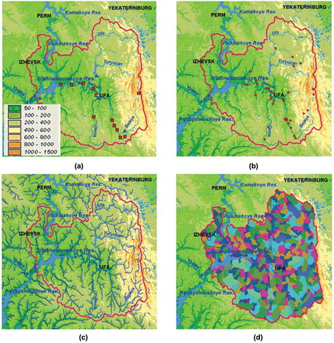
The model set-up for the catchment area and river network of the NKR was performed using the specific GIS tool Ecomag Extension (Motovilov 2016b), using digital thematic maps of the region: a digital elevation model (DEM, Fig. 4(a)), hydrographic network, soils and landscapes. First, a tree-type structure of the river network was constructed based on the DEM, and the boundaries of elementary watersheds were determined. The essence of this procedure is construction of streamline and pathline fields, and fields of flow accumulation based on a DEM. The cells with large values of flow accumulation form the model hydrographic network. After that, a procedure for the partition of the basin into elementary watersheds, representing partial drainage areas between the nodes (tributary confluence points) of the river network, was applied. These elementary watersheds are the smallest spatial elements used to simulate processes in the model.

Figure 4. Location of monitoring gauges and maps used for the model set-up for the Nizhnekamskoe Reservoir basin: (a) digital elevation model (DEM), hydrological gauges (triangles) and points of wastewater discharge (squares); (b) hydrochemical monitoring gauges; (c) schematization of the river network; and (d) sub-basins delineated based on the DEM.

The second stage of the river network construction is the structure–hydrographic analysis of the channel network. The Ecomag Extension tool uses two approaches for possible coding of the order of tributaries. In the first approach, according to the Shreve method, all streams that have no tributaries are assigned the first order. The order of the streams increases from the source to the mouth. At the confluence of two streams, their orders are added, and the sum is assigned to the downstream stream segment. In the second approach, which is used most often in Russia, the river orders are coded in another manner. The main river is assigned the zero order, its tributaries are assigned first order, those flowing into the first-order tributaries are assigned second order, and so on. The second coding procedure is algorithmically implemented in the ECOMAG-HM model for water and pollution routing in a branching river system.

At the final stage, data on the structure of the elementary watersheds and river network are transferred to the ECOMAG-HM model system, where the necessary model parameters of relief, soil, vegetation, etc. from appropriate databases are assigned to each elementary watershed. Overall, 503 elementary watersheds were delineated in the NKR watershed (Fig. 4(d)), with an average area of about 400 km². In addition to the main river, the modelled river network includes 50 first-order tributaries, 131 second-order ones, 63 third-order ones, and eight fourth-order tributaries (Fig. 4(c)).

2.4 Input data and boundary conditions

Data from 56 meteorological stations were used to specify the boundary conditions for the ECOMAG-HM model in the form of daily fields of weather characteristics (precipitation, air temperature and humidity) in the watershed area for the period 1978–2013.

Data on the daily water discharge at five gauges (Fig. 4(a)) were used to calibrate the model parameters and to test the hydrological submodel. An additional test was carried out by comparing the map of the simulated mean annual runoff in the basin with the map from SNIP (1985). The latter is usually used in Russia for determination of the hydrological characteristics in the design of hydraulic structures on rivers in the absence of hydrometric observations. This map was created as a contour map of the mean annual runoff for the former Soviet Union using measured streamflow data from about 6000 gauging stations. The streamflows at these gauging stations were considered to be natural (i.e. unaffected by upstream reservoirs) and representative of local conditions of runoff generation. For this study, the contours of mean annual runoff (SNIP 1985) were digitized and interpolated to produce a smooth grid using a GIS, and the mean annual runoff for each elementary watershed in the NKR area was estimated.

The initial conditions in the hydrochemical submodel for the spatial distribution of copper concentrations in soils were specified based on a map of copper concentrations in the ploughed layer of soils in the Republic of Bashkortostan, provided in the Atlas (Yaparov 2005). For adjacent administrative units a simple extrapolation of data was applied.

Unfortunately, no spatially-distributed data on copper concentrations in precipitation were available to specify the upper boundary conditions for the hydrochemical submodel. Therefore, a constant concentration of copper in precipitation was specified based on the weighted mean concentrations in Chernogayeva (2017). In a similar manner, copper concentration in the confined groundwater, which feeds perched water in the aeration zone, was specified as a constant value derived from data in Abdrakhmanov et al. (2007). The intensity of dry deposition of the atmospheric pollutants to the land surface was taken to be 0, due to the lack of any measurement data on it.

Data on the point anthropogenic sources of river water pollution by copper were taken from the information on copper discharge with wastewater in the 12 largest municipalities (Fig. 4(a)), provided in the state annual statistical environmental reports of industry, settlements and communal services. It should be noted that there is an opinion among experts that the reliability of these data is not high. This can be seen from the balance of hydrochemical data on the rivers before and after point sources of pollution (Fashchevskaya et al. 2006).

In addition, data on copper concentrations in river water at 34 stations of the Russian State Monitoring Survey (Fig. 4(b)) were used to calibrate the model parameters and to test the hydrochemical submodel. As a rule, copper concentrations at the gauges were measured on a monthly basis. The monitoring data on wasterwater discharge and copper concentrations in river water were collected over the period 2004–2007. Due to the short series of hydrochemical observations, the calibration was performed for all four years of observations without validation on independent data.

2.5 Model parameters

The hydrological submodel of ECOMAG-HM contains about 20 parameters. Most of them are physically meaningful and can be assigned from the regional reference books on properties of soils, landscapes and other data sources, or derived through available maps of land cover characteristics (Motovilov et al. 1999a, 1999b, Gelfan et al. 2015). The values for some of the most sensitive parameters (vertical and horizontal saturated hydraulic conductivities of soils, evaporation index in the Dalton formula, degree-day factor of snowmelt, etc.) were first specified using a step-by-step model calibration procedure against data on fields of soil moisture content and snow-water equivalent (available for the whole Volga River basin) over a long period (Motovilov et al. 2016b). Next, these parameters were corrected by calibration against the daily runoff hydrographs at the gauging stations in the study area. Additionally, the parameter of the elevation gradient for precipitation was calibrated against the difference between the simulated and estimated maps of the mean annual specific runoff in the basin.

The most sensitive parameters of the hydrochemical submodel are the sorption equilibrium constant of the Henry isotherm in soils, and the parameter accounting for metal exchange between the water mass and bottom sediments in rivers. The initial value of the former was chosen using data in Sauve et al. (2003). In addition, corrections were introduced for the values of copper concentrations in precipitation and confined groundwater. All these parameters were calibrated against data on copper concentrations in river water at 34 gauging stations of hydrochemical monitoring.

3 Results and discussion

3.1 Testing the hydrological module

The parameters of the hydrological submodel for the NKR watershed were calibrated against runoff hydrographs at five gauges over the period 2001–2007, and validated over the period 2008–2013. For that, the Nash-Sutcliffe efficiency criterion (NSE) for the daily hydrographs, and the PBIAS criterion, which characterizes the long-term differences of the observed annual runoff volumes against the simulated ones (in %), were applied. In addition, the hydrological submodel was validated against data on the hydrographs of lateral inflow into the NKR over the period 1978–2000. The results of tests for the periods of calibration and validation of the model are presented in Table 1, which shows that the agreement between the simulated and measured values of runoff characteristics is satisfactory (Moriasi et al. 2007).

Table 1. Statistical criteria of the daily and annual simulated runoff in comparison with the observed runoff for periods of calibration and validation of the model.

River, gauge	Drainage area (km^2)	Calibration		Validation
		NSE	PBIAS (%)	NSE	PBIAS (%)
Nugush, Nugush	2 870	0.70	18.6	0.71	12.8
Ufa, Pavlovsk	46 500	0.85	–7.7	0.67	–15.9
Belaya, Ufa	100 000	0.89	6.7	0.88	7.7
Belaya, Birsk	121 000	0.80	1.6	0.86	–5.4
Nizhnekamskoe Reservoir, Naberezhnye Chelny	184 400	0.86	–0.5	0.75	–3.6

The runoff characteristics in the rivers not covered by hydrometric observations were evaluated using mapping of the mean annual specific runoff (MASR). The method used to compile the map was as follows. Data from meteorological stations were used to construct daily fields of weather characteristics in the whole drainage area of the basin, and the hydrological submodel of ECOMAG-HM was applied to simulate runoff in the nodes (centres of gravity) of the elementary watersheds over many years. After that specific runoff (L s⁻¹ km⁻²) was used to calculate the MASR values and put them on a map.

Figure 5(a) and (b) shows maps of MASR estimated in SNIP (1985) and simulated by our model. As one can see from the maps, the spatial distributions of the fields of specific runoff are similar: a zone of low specific runoff is located in the southwestern part of the basin, and a zone of high values in the eastern part. The fields of specific runoff on the two maps differ in sub-areas of the NKR watershed by not more than one step in the legend gradations. The estimated values of the specific runoff vary within the range 3.8–14.0 L s⁻¹ km⁻², whereas the range of simulated values is 2.8–15.5 L s⁻¹ km⁻². The values of the estimated and simulated specific runoff, averaged over the NKR watershed area, are 6.88 and 6.95 L s⁻¹ km⁻², respectively, and the volumes of the average annual inflow into the NKR (integrals of the fields of the specific runoff values over the area) are 40.4 and 40.7 km³, respectively. The difference between these values, obtained by a cartographic method, and the runoff volume at the outlet section, estimated from hydrometric data (36.5 km³), is about 10%, a value that falls within the admissible error limits (Moriasi et al. 2007).

Figure 5. Mapping of river runoff characteristics in the Nizhnekamskoe Reservoir basin: (a) estimated and (b) simulated maps of the mean annual specific runoff (L s⁻¹ km⁻²); (c) relative errors in estimation of specific runoff; and (d) simulated mean annual water discharge in the river system (m³ s⁻¹).

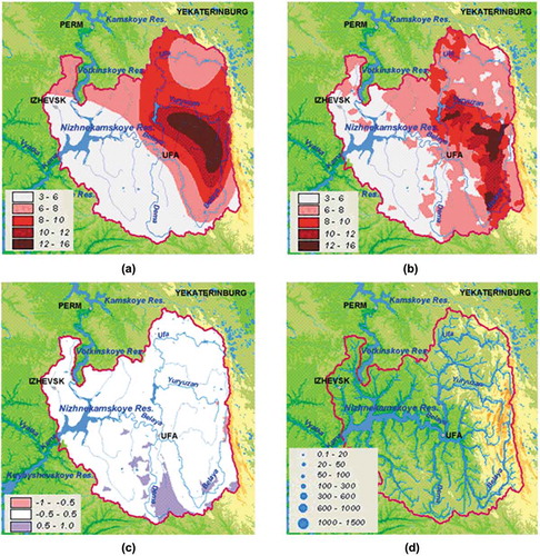
For a more detailed estimation of errors in the field of simulated specific runoff, Figure 5(c) depicts the field of relative errors calculated for each cell of a 1 km × 1 km grid in the river basin by dividing the difference between the estimated and simulated specific runoff values by the estimated value. As can be seen from this map, the relative errors fall between −0.5 and 0.5 almost everywhere in the river basin. In addition to the model errors, another possible source of errors is lack of reliable data of hydrometric observations for the construction of the map of the estimated MASR (SNIP 1985). For example, Voskresenskiy (1962) used data from 5690 gauges for the development of one of the most detailed maps of specific runoff for the USSR territory, and half of these gauges were in operation for less than 5 years, which is far from long enough for estimating reliable average long-term runoff characteristics.

The simulation results of the hydrological submodel of ECOMAG-HM were also analysed with the use of GIS for all elements of the modelled river network. Figure 5(d) shows the distribution of the simulated mean annual water discharge in the river system of the NKR watershed over 1979–2013. The thickness of the curve corresponds to water discharge in the river network in accordance with the legend.

3.2 Testing the hydrochemical submodel

The copper concentrations were simulated in the river network of the NKR watershed at a daily time step using the hydrochemical submodel ECOMAG-HM, and the simulated and measured concentrations were compared. According to Moriasi et al. (2007), the agreement of the modelling results with episodic data of measurements cannot be tested using strict statistical criteria adopted in hydrological practice, such as the Nash-Sutcliffe efficiency criterion. In such a case, we can compare the balance estimates based on simulation outputs and measurement data averaged over long periods. Besides, the agreement between the simulated and measured concentrations can be assessed by comparing differences between them with the estimated measurement error of hydrochemical concentrations. At the confidence level of p = 0.95, the error of copper concentration measurement within its variation range is about 50% (MUK 2003).

Figure 6(a) and (b) shows examples of the comparison of simulated copper concentrations on a daily basis with data of episodic measurements at two hydrochemical monitoring stations. The comparison shows that, in most cases, the discrepancy between the calculated and measured concentrations is comparable with the measurement errors.

Figure 6. Observed (green) and simulated (red) copper concentrations (µg L⁻¹) in river water at the hydrochemical monitoring gauges over the period 2004–2007: (a, b) daily dynamics; (c, d) average intra-annual concentrations; (e) long-term mean annual concentrations at the hydrochemical monitoring gauges in the Belaya River.

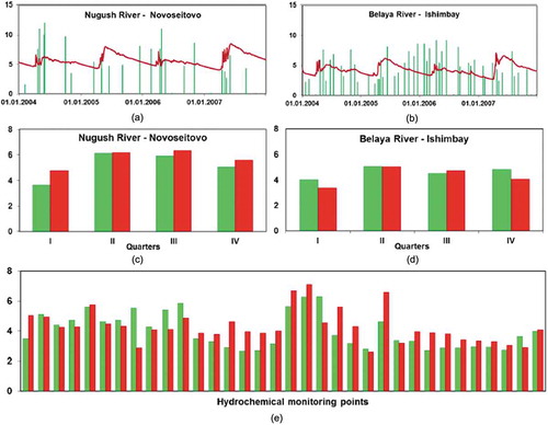
Figure 6(c) and (d) depicts the simulated and observed intra-annual copper concentrations for the same two stations, averaged over three months in four years. However, correlation analysis for all 34 gauge stations showed that the correlation coefficient between the simulated and measured averaged values was statistically significant (R = 0.55) only for the spring period, when maximum values of copper concentration occur. The long-term mean annual copper concentrations are presented in Figure 6(e) for 34 hydrochemical monitoring points on the river network in the order of their location from the upper reaches of the Belaya River toward its inflow into the NKR. It shows that the model adequately reproduces spatial differences in copper concentrations in the drainage basin, and the coefficient of correlation between the observed and simulated mean annual values is 0.58.

3.3 Spatio-temporal dynamics of copper washoff to the river network

The modelling results were used to analyse the spatio-temporal dynamics of copper washoff to the river network also in areas of the NKR watershed not covered by the hydrochemical observations. The maps of the mean annual specific copper washoff into the river network by surface and subsurface flows as well as by total flow were created based on the initial data and simulation outputs. The analysis of maps presented in Figure 7 shows that two components of the mean annual specific copper washoff, with subsurface flow (Fig. 7(d)) and with total water flow (Fig. 7(b)), are closely correlated with the initial spatial distribution of copper concentrations in soils (Fig. 7(a)). Higher values of the total washoff are simulated in the eastern part of the river basin, with peaks in the northeastern part. The second important factor affecting the spatial distribution of copper washoff is the rate of water exchange. A comparison of the maps of copper washoff (Fig. 7(b) and (d)) with the map of mean annual specific runoff (Fig. 5(b)) shows that the higher specific water runoff at the southeastern margin of the basin (the upper reaches of the Belaya River) leads to higher specific copper washoff, though no anomaly can be seen in the distribution of copper concentrations in soils of this area.

Figure 7. Mapping of copper washoff characteristics in the Nizhnekamskoe Reservoir watershed: (a) initial copper concentrations (mg kg⁻¹) in soils, based on Yaparov (2005); (b), (c) and (d), respectively, total, surface and sub-surface simulated mean annual specific copper washoff (g year⁻¹ km⁻²) over the period 2004–2007; (e) ratio of the surface and subsurface specific washoff of copper; and (f) simulated mean annual copper concentrations in the river water (µg L⁻¹).

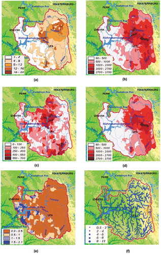
Figure 7(c) shows copper washoff with the surface runoff component. The values are generally low in the eastern part of the basin (due to higher permeability of soils in the piedmont of the southern Urals) and in river valleys. Comparison of the surface (Fig. 7(c)), subsurface (Fig. 7(d)) and total (Fig. 7(b)) washoff components shows that the copper transport with surface runoff is relatively small. This can be seen better in Fig. 7(e), which shows the ratio of copper washoff with surface and subsurface flows in the basin. This map indicates that the surface component of copper washoff does not exceed one-half of the subsurface component in most parts of the basin. Only in a few small sub-areas of the western part of the basin is the surface component of copper washoff larger than the subsurface component; this may be due to the low local concentrations of copper in soils (Fig. 7(a)).

Figure 7(f) provides a map of the simulated mean annual copper concentrations in river water, obtained by averaging the daily concentrations of copper in the elements of the modelled river network over the period 2004–2007. The model estimates show that river water quality in the NKR watershed fails to meet the requirements of water bodies used for fisheries, and the mean annual copper concentration in river water exceeds the MAC by two to eight times. The simulated copper concentrations are maximal (up to 8 µg L⁻¹) in the tributaries of the middle reaches of the Ufa River, i.e. in the areas with the maximum values of MASR (Fig. 5(b)). High concentrations can also be seen in the middle reaches of the Belaya River and its tributaries. The lowest concentrations were simulated in the lower reaches of the Belaya River.

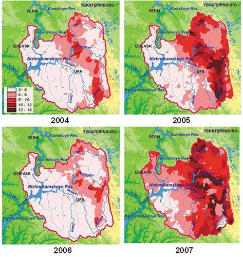
The maps of annual precipitation and specific runoff over the period 2004–2007 are shown in Figures 8 and 9, respectively, for a more detailed analysis of the processes. As one can see from these maps, on the whole the spatial distributions of the fields of characteristics are similar: zones of low values are located in the southwestern part of the basin, and zones of maximum values are confined mainly to areas of high relief in the central and eastern parts of watershed on the spurs of the southern Urals (see Fig. 4(a)). In Figure 8 the inter-annual variability of annual precipitation may be seen: in 2004, 2006 and 2007 the fields are quite similar (mean annual precipitation averaged over the area of watershed was 642, 657 and 627 mm, respectively), but in 2005 precipitation was very low (460 mm).

Figure 8. Mapping of annual precipitation (mm year⁻¹) over the period 2004–2007.

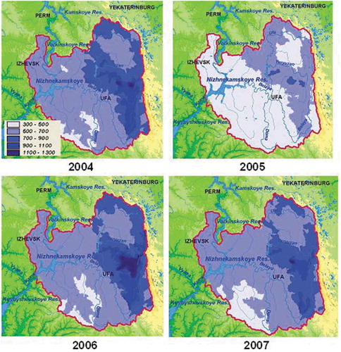
Figure 9. Mapping of simulated specific runoff (L s⁻¹km⁻²) over the period 2004–2007.

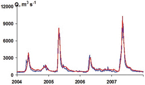
Figure 9 shows the inter-annual variability of specific runoff fields. The lowest values of the watershed MASR averaged over the area were observed in 2004 and 2007 (5.4 and 5.1 L s⁻¹ km⁻², respectively) and the highest values in 2005 and 2007 (7.0 and 9.0 L s⁻¹ km⁻², respectively). Comparison of the maps in Figures 8 and 9, as well as average annual precipitation and specific runoff values for the period 2004–2006, does not show a temporal correlation between these characteristics. This is confirmed by Figure 10, which shows a comparison of the measured and simulated lateral inflow hydrograph in the NKR for that period. It is shown that the spring runoff in years with maximum annual precipitation (2004 and 2006) is small, and the hydrograph of spring runoff in 2005 with minimum annual precipitation is high. This is due to the fact that winter soil moisture has a significant impact on the spring runoff in addition to snow water equivalent. In the years with small winter soil moisture a significant part of snowmelt waters is spent on replenishment of moisture reserves in soil and groundwater, and spring flood runoff turns out to be insignificant. The reverse pattern is observed in years with high soil moisture. The simulated mean watershed soil moisture supply, averaged over the area, in the upper 50-cm layer on 1 January for the years 2004–2007 was 71, 124, 67 and 113 mm, respectively. This explains the low spring runoff (and annual specific runoff) in years with dry soils (2004 and 2006) and high runoff in years with significant winter soil moisture (2005 and 2007).

Figure 10. Observed (blue) and simulated (red) daily discharges of lateral inflow into the NKR over the period 2004–2007.

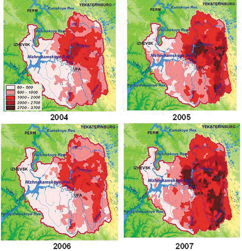
Figure 11 shows the maps of specific copper washoff over the period 2004–2007. Comparison of these maps with the maps of annual precipitation and specific runoff (Figs 8 and 9) shows a close spatial-temporal correlation with the latter. Maximum values of the mean specific copper washoff, averaged over the area of the watershed, are observed in years with maximum specific runoff (2005 and 2007).

Figure 11. Mapping of simulated annual specific copper washoff (g year⁻¹ km⁻²) over the period 2004–2007.

3.4 Assessment of the contribution of different components to the total copper load

The balance model simulations were used to estimate the contributions of different components to the total copper load from the NKR watershed, including the effects of point anthropogenic sources for the period 2004–2007. The results are summarized in Table 2. The actual annual load of copper from the catchment into the NKR (the last column in Table 2) was estimated by multiplying the observed annual discharge of inflow into the NKR by the observed average annual concentration of copper at the last monitoring station on the Belaya River (Dyurtuli gauge).

Table 2. Simulated components of copper load (t year⁻¹) from the NKR watershed and the actual total copper load into the NKR in the period 2004–2007.

	Copper load				Total Cu load into NKR
Year	With surface water flow	With subsurface water flow	Actual load of Cu by wastewater	Copper settling onto riverbed	Simulated	Actual
2004	25	130	2.3	82	75	127
2005	50	192	2.4	106	138	166
2006	18	123	2.3	78	65	54
2007	68	252	2.1	130	192	129
Mean annual	40.3	174.3	2.3	99	118	119

The following conclusions can be drawn from Table 2:

1. The total copper inflow into the NKR consists of about 80% subsurface and 20% surface washoff, on average.

2. On average, about 45% of copper washed out from the drainage area is bound to sediments and settled to bottom deposits in the river network.

3. The share of copper entering the river network with wastewater discharge is small, accounting for about 1% of the total copper washed off from the drainage watershed area.

4. Comparison of the simulated and actual total copper inflow into the NKR shows that the model adequately reproduces temporal copper dynamics in the watersheds and trends. The differences between these values are due to both the model errors and the low accuracy in determining the average annual concentrations of copper in river water.

4 Conclusions

In this study, the Nizhnekamskoe Reservoir (NKR) watershed was used as an example to demonstrate the abilities of the ECOMAG-HM model in evaluating the hydrological and hydrochemical characteristics of large river basins based on standard hydro-meteorological data, digital maps, databases of hydrophysical and geochemical characteristics of soils and landscapes, and characteristics of anthropogenic load on the rivers.

The verification of the hydrological submodel against data on river runoff at five gauges showed a satisfactory agreement between the simulated and observed runoff characteristics. Comparison of the simulated map of mean annual surface runoff (MASR) in the NKR watershed area with the estimated map given in SNIP (1985) showed that the variation ranges of the simulated and observed specific runoff are very similar, as well as the average values of runoff over the whole watershed area, and the volumes of average annual runoff. The relative errors in the simulated specific runoff do not exceed 50% in most parts of the watershed.

Testing of the hydrochemical submodel showed that it adequately reproduces the average intra-annual variations of copper concentrations in river water and spatial variations of mean annual copper concentrations at various hydrochemical monitoring points. The model reflects the inter-annual dynamics of copper inflow into the NKR quite well. The model enables assessment of copper pollution dynamics with a higher spatial and time resolution than the existing hydrochemical monitoring network allows. The quantitative estimates and maps depict the mean annual specific copper washoff with the surface, subsurface and total water flows in the watershed area. It was shown that the subsurface component predominates in the total copper transport in most parts of the drainage area, and in only a few places in the western part the surface component of copper transport is larger.

The contributions of the direct anthropogenic (wastewater) and diffuse components to the total copper washoff in the NKR watershed were assessed. The model balance estimates averaged over the basin area showed that the copper washoff into the river network from the soil-ground stratum accounts for about 80% of the total copper washoff, and the rest 20% comes with surface runoff. About 45% of the total copper washed out from the drainage basin into the river network accumulates in the riverbed with sediments. According to our estimates based on published data, the direct anthropogenic component of copper pollution of river water from wastewater (combined industrial and municipal components) is relatively small, accounting for about 1% of the total copper inflow into the NKR from the watershed.

The obtained results can be of use in scientific-methodological studies and applications for assessing diffuse pollution and the contribution of the direct anthropogenic component to river water pollution, as well as for planning measures for water quality control of water resources in large river basins.

Acknowledgments

We would like to thank Dr Valentina Krysanova for her helpful and constructive advice, which helped to improve the clarity of the arguments presented in this paper.

Disclosure statement

No potential conflict of interest was reported by the authors.

Additional information

Funding

The simulation of hydrochemical flow was supported by the Russian Scientific Foundation [project no. 17-77-30006]. The simulation of river runoff fields was supported by the Russian Foundation for Basic Research [project no. 16-05-00864].

References

- Abbaspour, K.C., et al., 2015. A continental-scale hydrology and water quality model for Europe: calibration and uncertainty of a high-resolution large-scale SWAT model. Journal of Hydrology, 524, 733–752. doi:10.1016/j.jhydrol.2015.03.027
- Abdrakhmanov, R.F., Chalov, Y.N., and Abdrakhmanova, E.P., 2007. Presnye podzemnye vody Bashkortostana [Fresh groundwater in Bashkortostan]. Ufa: Informreklama.
- Barenboim, G.M., et al., 2013. On the problems of water quality in Russia and some approaches to their solution. IAHS Publ., 361, 77–86.
- Bashkortostan: Kratkaya entsiklopediya [The Republic of Bashkortostan: brief ensyclopedia]. 1996. Ufa: Nauchnoe Izd. “Bashkirskaya entsiklopediya”.
- Bedient, P.B., Lambert, J.L., and Springer, N.K., 1980. Stormwater pollutant load runoff relationships. Journal Water Pollution Control Federation, 52 (9), 2396–2404.
- Chernogayeva, E.M., 2017. Tendentsii i dinamika sostoyaniya i zagryazneniya okruzhayushchey sredy v Rossiyskoy Federacii po dannym mnogoletnego monitoringa za poslednie 10 let. Analiticheskiн obzor [Tendencies and dynamics of the state and pollution of the environment in the Russian Federation according to the data of long-term monitoring for the last 10 years. Analytical review]. resp. ed.. Moscow: Rosgidromet.
- Ezhegodnik. Zagryaznenie pochv v Rossijskoj Federacii promyshlennymi toksikantami v 2010 godu [Yearbook. Soil pollution in the Russian federation by industrial toxicants in 2010], 2011. Obninsk: GU “VNIIGMI-MTsD”.
- Fashchevskaya, T.B., Krasnogorskaya, N.N., and Rogozina, T.A., 2006. O vozdeystvii predpriyatiya “Ufavodokanal” na kachestvo vody reki Beloy. Materialy mezhdunarodnoy nauchnoy konferentsii “Ekologicheskie i gidrometeorologicheskie problemy bolshih gorodov i promyshlennyh zon” [On the impact of the enterprise “Ufavodokanal” on the water quality of the Belaya River. Proceedings of the international scientific conference “ecological and hydrometeorological problems of large cities and industrial zones”]. St. Petersburg: Izd. RSHU, 80–82.
- Fashchevskaya, T.B., Motovilov, Y.G., and Shadiyanova, N.B., 2018. Natural and anthropogenic variations of the concentrations of iron, copper and zinc in water streams of the Republic of Bashkortostan. Water Resources, 45 (6), 873–886. doi:10.1134/S0097807818060064
- Fuchs, S., et al., 2017. Modeling of regionalized emissions (MoRE) into water bodies: an open-source river basin management system. Water, 9 (4), 239. doi:10.3390/w9040239
- Galvan, L., et al., 2009. Application of the SWAT model to an AMD-affected river (Meca River, SW Spain). Estimation of transported pollutant load. Journal of Hydrology, 377, 445–454. doi:10.1016/j.jhydrol.2009.09.002
- Gao, L. and Li, D., 2014. A review of hydrological/water-quality models. Frontiers of Agricultural Science and Engineering, 1 (4), 267–276. doi:10.15302/J-FASE-2014041
- Gelfan, A., et al., 2015. Testing the robustness of the physically-based ECOMAG model with respect to changing conditions. Hydrological Sciences Journal, 60 (7–8), 1266–1285. doi:10.1080/02626667.2014.935780
- Gelfan, A.N. and Motovilov, Y.G., 2009. Long-term hydrological forecasting in cold regions: retrospect, current status and prospects. Geography Compass, 3/5, 1841–1864. doi:10.1111/j.1749–8198.2009.00256.x
- Gosudarstvennyj doklad “O sostoyanii i ohrane okruzhayushchej sredy Respubliki Bashkortostan v 2004 godu” [State report on the environmental state and protection in the Republic of Bashkortostan in 2004], 2005. Ufa: Minekologii Respubliki Bashkortostan.
- Harmel, R.D., et al., 2014. Evaluating, interpreting, and communicating performance of hydrologic/water quality models considering intended use: a review and recommendations. Environmental Modelling & Software, 57, 40–51. doi:10.1016/j.envsoft.2014.02.013
- Hesse, C. and Krysanova, V., 2016. Modeling climate and management change impacts on water quality and in-stream processes in the Elbe river basin. Water, 8 (2), 40. doi:10.3390/w8020040
- Knisel, W.G., ed., 1980. CREAMS: a field scale model for chemical, runoff and erosion from agricultural management systems. In: USDA conservation research report, No. 26. Washington: Dept. of Agriculture, Science and Education Administration.
- Krysanova, V., et al., 2009. Water quality modelling in mesoscale and large river Basins. In: Encyclopedia of life support systems (EOLSS), 2: hydrological systems modeling. Isle of Man: Eolss Publishers, 11–48.
- Leebai, N., Leungprasert, S., and Sirivittayaprakron, S., 2016. Organic pollutants and heavy metals transport in the lower Chaophraya Basin Using SWAT model. International Journal of Advances in Science Engineering and Technology, 2, 21–25.
- Linnik, P.N. and Nabivanets, B.I., 1986. Formy migratsii metallov v presnyh poverhnostnyh vodah [Forms of migration of metals in fresh surface waters]. Leningrad: Gidrometeoizdat.
- Maistrenko, V.N., Khamitov, R.Z., and Budnikov, G.K., 1996. Ekologo-analiticheskii monitoring superekotoksikantov [Ecological-analytical monitoring of superecotoxicants]. Moscow: Khimiya.
- Moriasi, D.N., et al., 2007. Model evaluation guidelines for systematic quantification of accuracy in watershed simulations. Transactions of the ASABE, 50 (3), 885–900. doi:10.13031/2013.23153
- Motovilov, Y.G., 2016a. Hydrological simulation of river basins at different spatial scales: 1. Generalization and averaging algorithms. Water Resources, 43 (3), 429–437. doi:10.1134/S0097807816030118
- Motovilov, Y.G., 2016b. Hydrological simulation of river basins at different spatial scales: 2. Test results. Water Resources, 43 (5), 743–753. doi:10.1134/S0097807816050092
- Motovilov, Y.G., 2017. Modeling fields of river runoff (a case study for the Lena river Basin). Russian Meteorology and Hydrology, 42, 121–128. doi:10.3103/S1068373917020066
- Motovilov, Y.G., et al., 1999b. Validation of a distributed hydrological model against spatial observation. Agricultural and Forest Meteorology, 98–99, 257–277. doi:10.1016/S0168-1923(99)00102-1
- Motovilov, Y.G., 2013. ECOMAG: a distributed model of runoff formation and pollution transformation in river basins. IAHS Publ., 361, 227–234.
- Motovilov, Y.G., et al., 1999a. ECOMAG: regional model of hydrological cycle. Application to the NOPEX region. Department of Geophysics, University of Oslo.
- MUK 4. 1.1258-03, 2003. Metody kontrolya. Khimicheskie factory. Izmerenie massovoi kontsentratsii medi fluorimetricheskim metodom v probakh pit’evoi vody i vody poverkhnostnykh i podzemnykh istochnikov vodopol’zovaniya [Control methods. Chemical factors. Measuring copper mass concentration by fluorimetriс methods in samples of drinking water and water from surface and subsurface sources of water use]. Moscow: Minzdrav Rossii.
- Santhi, C., et al., 2008. Spatial calibration and temporal validation of flow for regional scale hydrologic modeling. Journal of the American water resources association, 44, 829–846. doi:10.1111/j.1752-1688.2008.00207.x
- Sauvé, S., et al., 2003. Solid-solution partitioning of Cd, Cu, Ni, Pb and Zn in the organic horizons of a forest soil. Environmental science & technology, 37 (22), 5191–5196. doi:10.1021/es030059g
- SNIP-2.01.14-83, 1985. Opredelenie raschetnyh gidrologicheskih harakteristik [Construction standards and regulations, determining design hydrological characteristics]. Moscow: Stroiizdat.
- Vink, R. and Peters, S., 2003. Modelling point and diffuse heavy metal emissions and loads in the Elbe basin. Hydrological processes, 17, 1307–1328. doi:10.1002/hyp.1286
- Voskresenskiy, K.P., 1962. Norma i izmenchivost’ godovogo stoka rek Sovetskogo Soyuza [Normal annual runoff and its variations in Rivers in the Soviet Union]. Leningrad: Gidrometeoizdat.
- Yang, Y.S. and Wang, L., 2010. A review of modelling tools for implementation of the EU water framework directive in handling diffuse water pollution. Water Resources Management, 24, 1819–1843. doi:10.1007/s11269-009-9526-y
- Yaparov, I.M., 2005. Atlas Respubliki Bashkortostan [Atlas of the Republic of Bashkortostan]. resp. ed. . Ufa: Kitap.
- Zhang, P., et al., 2013. Land use pattern optimization based on CLUE-S and SWAT models for agricultural non-point source pollution control. Mathematical and Computer Modelling, 58, 588–595. doi:10.1016/j.mcm.2011.10.061