Evaporation modelling by heuristic regression approaches using only temperature data

ABSTRACT

Accurate estimation of pan evaporation (E_pan) is very important in water resources management, irrigation scheduling and water budget of lakes. This study investigates the accuracy of two heuristic regression approaches, multivariate adaptive regression splines (MARS) and M5 model tree (M5Tree) in estimating pan evaporation using only temperature data as input. Monthly minimum temperature, maximum temperature and E_pan data from three Turkish stations were used, with month number (periodicity information) added as input to see its effect on estimation accuracy. The models were compared with the calibrated Hargreaves-Samani (CHS), Stephens-Stewart (SS) and multiple linear regression methods. Three different train-test splitting strategies (50%–50%, 60%–40% and 75%–25%) were employed for better evaluation of the applied methods. The results show that the MARS method generally estimated monthly E_pan with higher accuracy compared to the M5Tree, CHS and SS methods. When extraterrestrial radiation, calculated from Julian date and latitude information, was used as input to the SS instead of solar radiation, satisfactory estimates were obtained. A positive effect on model accuracy was observed when involving periodicity information in inputs and increasing training data length.

KEYWORDS:

• pan evaporation
• estimation
• MARS
• M5 model tree
• Stephens-Stewart

Editor S. Archfield Associate editor N. Verhoest

Introduction

Pan evaporation (E_pan) is a key variable in water resources management, water budget of lakes and reservoirs, and crop water requirements. Therefore, exact quantification of E_pan is a prerequisite, since it has significant impacts on hydrological processes. Evaporation from water reservoirs will vary depending on several factors, including climate, reservoir characteristics and use practices (Wurbs and Ayala 2014). Direct measurement of evaporation using a standard pan evaporimeter is an effective tool for assessing the water cycle of lakes and reservoirs and has been adopted worldwide, as well as being recommended by the World Meteorological Organization (WMO) (Chu et al. 2010). When conducted properly, a direct measurement approach can provide an exact and faithful continuous record and will be the best procedure. Indirect estimation of E_pan using models is an alternative and attractive tool for providing quantification of evaporation. Several studies worldwide have reported the successful use of various kinds of models for estimating evaporation from surface water, and there are at least two categories of models: (1) physically-based (climate-based models) and (2) artificial intelligence (AI)-based models.

Figure 1. Locations of the stations used in the study.

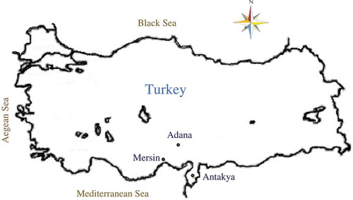
Figure 2. Structure of the MARS model (after Deo et al. 2017).

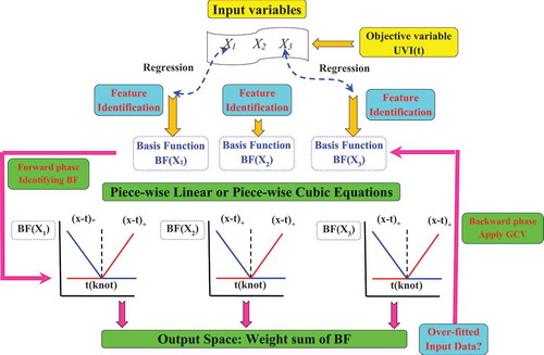
Figure 3. Structure of the M5Tree model (after Deo et al. 2017, Sanikhani et al. 2018).

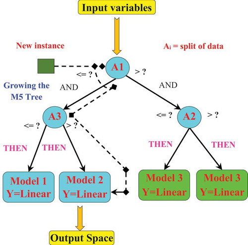
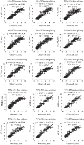
Figure 4. Observed and estimated E_pan by the MARS, M5Tree, CHS, SS and MLR methods in the test period – Adana station.

Kisi et al. (2016) compared three machine learning models – classification and regression tree (CRT), chi-squared automatic interaction detector (CHAID) and the multilayer perceptron neural network (MLPNN) – for modelling daily E_pan using climatic variables from two weather stations in Turkey. They demonstrated that MLPNN is slightly superior to the two other models. Wang et al. (2017a) conducted a comparative study between six data-driven techniques (DDT) for predicting monthly E_pan using large datasets at different climates in China. They selected five meteorological variables – air temperature (T_mean), wind speed (U), sunshine hours (SH), solar radiation (SR) and relative humidity (RH) – and compared the following models: MLPNN, generalized regression neural network (GRNN), fuzzy genetic (FG), least square support vector machine (LSSVM), multivariate adaptive regression spline (MARS), and adaptive neuro-fuzzy inference systems with grid partition (ANFIS-GP). In addition, two standard regression models were used: multiple linear regression (MLR) and the Stephens-Stewart model (SS; Stephens and Stewart 1963). According to the results obtained, the MLPNN was broadly more accurate at the majority of the stations. In other studies, Wang et al. (2017b, 2017c) compared FG, LSSVM, MARS, the M5 model tree (M5Tree) and the MLR models for predicting daily E_pan using T_mean, SH, RH, U and the surface temperature (T_s). They tested two scenarios: local inputs and a cross-validation scenario. According to the results obtained, overall the FG and LSSVM performed best, especially in the case of limited input variables. The high-order response surface method (HORS), a new model for monthly E_pan, was introduced by Keshtegar and Kisi (2016) and applied using four meteorological variables (T_mean, SR, RH, U) in Turkey. Compared to the MLPNN, FG and the ANFIS models, the HORS method provided the best accuracy. Keshtegar and Kisi (2017) applied the hybrid response surface function (HRSF), a modified version of the HORS method, for predicting monthly E_pan in Turkey. Compared to the second-order response surface method (RSM), ANFIS and M5Tree models, they demonstrated that HRSF and HORS yielded superior results. Malik et al. (2017) compared four machine learning models: (a) co-active neuro-fuzzy inference system (CANFIS), (b) radial basis function neural network (RBFNN), (c) MLPNN and (d) self-organizing map neural network (SOM), for modelling monthly pan evaporation in India. The proposed data-driven models were compared to the climate-based models: the SS model and the Griffith (GF) model. Another of the few studies using the gamma test (GT) for selecting the best input combination of climatic variables for predicting E_pan was conducted by Malik et al. (2018), using six climatic variables as inputs – minimum and maximum air temperatures (T_min and T_max), morning and afternoon relative humidity (RH₁ and RH₂), wind speed (U) and sunshine hours (SH). Based on GT results, the RBFNN model with all six variables as inputs gave the best accuracy, the root mean square error (RMSE) of the multiple linear regression model (MLR) was considerably higher than that produced by the RBFNN model. A new data-driven model for daily E_pan was recently proposed by Adamala et al. (2018), who compared the generalized higher-order neural network (GHNN) with the generalized first-order neural network (GFNN) and generalized multiple linear regression (GMLR) models. The proposed models were employed for modelling daily E_pan in four different climatic regions in India: semi-arid, arid, sub-humid and humid. The researchers concluded and demonstrated the superiority of the GHNN compared to the GFNN and GMLR models.

Deo and Samui (2017) applied four data-driven models – LSSVM, Gaussian process regression (GPR), minimax probability machine regression (MPMR) and genetic programming (GP) – for predicting daily E_pan using several climatic variables, e.g. precipitation (P), U, mean solar exposure (S_t), T_min, T_max and daily SR. Comparison of the LSSVM model with GPR, MPMR and GP on the basis of the prediction accuracy showed that the LSSVM model was more accurate and gave a high correlation coefficient for the testing set, whereas the GP model was the worst. More recently, another data-driven model employed for predicting monthly E_pan was introduced by Eray et al. (2017): the dynamic evolving neural-fuzzy inference system (DENFIS). Compared to the multi-gene genetic programming (MGGP), based on the use of five climatic variables – T_max, T_min, U, SH and RH – collected at two climatic stations in Turkey, the authors demonstrated that the DENFIS performed better at one station, while the MGGP performed better at the second. Arunkumar et al. (2017) selected six daily meteorological variables – T_min, T_max, SH, U, RH and dew point temperature (T_dew) – for predicting daily E_pan using three AI models: the time-lagged recurrent neural network (TLRN), the M5Tree and the GP model. According to the results obtained, they demonstrated that the GP had the best prediction accuracy, followed by the TLRN model, while the M5Tree gave the lowest accuracy. Pammar and Deka (2017) used the GT method for selecting the best input combination of five meteorological variables – U, P, RH, SH and T_mean – and compared with two DDT for predicting daily E_pan in India. They compared the standard support vector regression (SVR) having three different kernel functions and the discrete wavelet transform–support vector regression (DWT-SVR) hybrid models. Based on the results, the authors demonstrated that the DWT-SVR provided the best accuracy compared to the SVR model, and DWT-SVR with radial basis function (RBF) as kernel function had the best prediction accuracy. Ghorbani et al. (2017) proposed a new hybrid model, the multilayer perceptron–firefly algorithm (MLP-FFA), for predicting daily E_pan in the arid regions of Iran. Using five meteorological variables – T_max, T_min, U, SH and RH – they demonstrated that the MLP-FFA model outperformed the MLPNN and the SVM models.

Several other studies (Kim and Kim 2008, Shiri et al. 2011, 2014, Kim et al. 2012) have compared one or more of the AI models reported above, using several meteorological variables at different time steps, and the results obtained have shown that AI models generally provided good accuracy. However, even though the aforementioned studies demonstrated an increased use of AI models, the most important point to note is that, generally speaking, these models require several inputs, i.e. U, RH, SH, T_mean, T_max and T_min, and among them the U, RH, SH and SR are the meteorological variables reported as the most significant factors influencing E_pan and involved in primary importance. Although T_max and T_min were used in several studies focused on modelling E_pan, to the best of our knowledge, no study in the literature has used temperature-based data-driven regression models to predict E_pan. Hence, this paper makes three main contributions to the related literature. Firstly, in this study, we propose the application of two temperature-based data-driven regression models – the MARS and M5Tree models – using only T_max and T_min as input variables, while most of the other studies in the literature used a mix of these two variables and several other meteorological variables. Secondly, for the first time in the SS model, we use extraterrestrial radiation, which is easily obtained from the Julian date and latitude information, instead of solar radiation. Thirdly, we demonstrate the effect of periodicity (month number) as an input variable for E_pan estimation using limited climatic inputs. In this study, we apply three different data-splitting strategies, whereas one splitting rule is generally reported in the related literature.

Materials and methods

Case study

The study uses monthly minimum and maximum temperatures (T_min and T_max) and pan evaporation (E_pan) measured at the stations Adana (37°00′N, 35°19′E; 27 m a.m.s.l.), Antakya (36°33′N, 36°30′E; 100 m a.m.s.l.) and Mersin (36°48′N, 34°38′E; 3 m a.m.s.l.) situated in the Mediterranean region of Turkey. The locations of the stations can be seen in Figure 1. This region has cool and rainy winters and hot and moderately dry summers. Annual rainfall ranges from 580 to 1300 mm. The Taurus Mountains are close to the coastal area and rain clouds cannot pass these mountains and drop their water on the coastal area (Sensoy et al. 2016). The study stations are operated by the Turkish Meteorological Organization. The data periods are 1960–2016, 1962–2015 and 1986–2016 for the Adana, Antakya and Mersin stations, respectively. Table 1 presents the statistical parameters of the climatic data used in the present study. The extraterrestrial radiation, R_a, of Antakya station has a high negative skewness. The E_pan data range of Antakya is higher than that of the Adana and Mersin stations. The correlations between dependent (T_min, T_max and R_a) and independent (E_pan) variables are smaller for Antakya compared to other two stations (Table 1).

Table 1. Statistical parameters of climatic data used in the study. T_min: minimum temperature; T_max: maximum temperature; R_a: extraterrestrial radiation; E_pan: pan evaporation. x_min, x_max, x_mean, S_x and C_sx are minimum, maximum, mean, standard deviation and skewness, respectively.

Station	Variable	xmin	xmax	xmean	Sx	Csx	Correlation with Epan
Adana	Tmin (°C)	–8.10	23.4	9.06	7.63	0.10	0.892
	Tmax (°C)	16.6	44.0	31.1	7.02	–0.40	0.856
	Ra (MJ/m^2)	15.5	41.7	29.3	9.34	–0.12	0.849
	Epan (mm)	0.50	10.1	4.27	2.31	0.34	1.000
Antakya	Tmin (°C)	–7.00	25.0	9.97	7.83	0.01	0.832
	Tmax (°C)	13.8	43.9	30.5	7.25	–0.54	0.751
	Ra (MJ/m^2)	16.0	41.6	30.7	8.88	–1.38	0.767
	Epan (mm)	0.80	13.2	4.85	2.47	0.45	1.000
Mersin	Tmin (°C)	–1.40	27.0	11.9	7.63	0.10	0.859
	Tmax (°C)	15.6	38.5	28.4	5.65	–0.41	0.782
	Ra (MJ/m^2)	15.7	41.6	29.4	9.26	–0.11	0.831
	Epan (mm)	0.70	8.10	3.47	1.73	0.42	1.000

Heuristic regression approaches

Multivariate adaptive regression splines model

The multivariate adaptive regression splines (MARS) model used in this study was developed by Friedman (1991). It has been used recently for suspended sediment load by Yilmaz et al. (2018), analysis of driver lane-keeping behaviour in rain (Ghasemzadeh and Ahmed 2018), forecasting natural gas consumption (Ozmen et al. 2018), electricity demand forecasting (AL-Musaylh et al. 2018), estimation of long-term monthly temperatures (Mehdizadeh 2018), mix design method for fly ash geopolymer concrete (Lokuge et al. 2018) and damage detection of structures (Ghiasi et al. 2018). In the MARS model, the dependent variable is linked to the independent variables in the form of a nonparametric regression formula, and the model is presented by a three terms: (a) the knots, (b) the spline function and (c) the basis functions (BF) (Friedman 1991). The main ideas behind the MARS model are as follows: on the one hand, the relationship between the independent and dependent variables does not necessarily have to be well known; on the other hand, the available information in the space of the independent variables is shared (divided) into various regions called knots, and for each knot a regression model is developed using a spline function, itself composed of one or more BFs that replace the original predictors (Abraham et al. 2001). The predicted value from the MARS model is based on a linear combination of the BF components involved in the space of the predictors and is summarized as follows:

(1) $Y=f\left(x\right)={\beta }_0+\sum _{m=1}^M{\beta }_m\mathrm{B}{\mathrm{F}}_m\left(X\right)$(1)

where β_m are unknown coefficients of the model determined during the iterative process, Y is the predicted variable (E_pan), BF are the basis functions used to fit the MARS model and composed of the original predictors, i.e. x_i (meteorological variables), and M is the total number of BFs (Friedman 1991, Ghasemzadeh and Ahmed 2018). According to Friedman (1991), the MARS model is built in two stages, a forward (selection) stage and a backward (pruning) stage (see Fig. 2). The forward stage is governed by a condition: the maximum number of BFs (M in Equation (1)) fixed at the beginning of the learning process must be reached. During the forward stage, an overfitted and very complex model is created taking into account all possible BFs, starting with a constant (BF(x) = 1) and ending with all possible BFs (Ozmen et al. 2018). The forward stage is achieved with a model composed of a very high number of BFs, which does not greatly influence the accuracy of the model and the capacity of generalization is not guaranteed. Hence, a second backward stage that eliminates and reduces the BFs with the lowest magnitude is needed in order to obtain an efficient MARS model. During this stage, the BF that least increases the error function is removed from the model and, at each iteration, the effect of the pruning process on prediction accuracy is examined; obviously the final pruned model, based on the backward stage, must still be capable of predicting the test data with high accuracy (Friedman 1991, Abraham et al. 2001). From a mathematical point of view, the backward pruning stage is realized based on the generalized cross-validation (GCV) (Friedman 1991, Abraham et al. 2001, Lokuge et al. 2018, Ozmen et al. 2018):

(2) $\mathrm{G}\mathrm{C}\mathrm{V}\left(M\right)=\frac{\frac{1}{N}\sum _{i=1}^N{\left(y_i-f\left(x_i\right)\right)}^2}{{\left(1-\frac{c\left(M\right)}{N}\right)}^2}$(2)

where N is the number of data, y_i is the desired value or the measured E_pan, f(x_i) is the calculated value of the pattern i, c(M) is the penalty factor, also called a complexity penalty function (Lokuge et al. 2018, Yilmaz et al. 2018). In this study, the MARS model was employed using the MatLab toolbox ARESLab (Jekabsons 2016a).

M5 model tree

The decision tree (DT) algorithm is based on the interaction between two kinds of nodes: a root (primary) node and a secondary node, which together form a tree (Li et al. 2018). The DT is a recursive partitioning method, which distributes the input space, containing the input variables, into several homogeneous subsets in terms of dependent variables, and identifies optimal rules called nodes (Hamze-Ziabari and Bakhshpoori 2018). The DT works with respect to two conditions: maximize the information and minimize the error in the branches of the tree (Quinlan 1992, Wang and Witten 1997). The M5 model tree (M5Tree) is inspired by the DT approach (Quinlan 1992) and is structured on several multiple linear regression models, each of which is specialized on one subset; the final model is composed of these individual sub-models. The M5Tree model is achieved in three stages (see Fig. 3): (a) DT induction (the building stage), (b) pruning the tree and (c) smoothing (Quinlan 1992, Wang and Witten 1997, Hamze-Ziabari and Bakhshpoori 2018). During the building stage, the model uses the standard deviation reduction (SDR) as the splitting criterion:

(3) $\mathrm{S}\mathrm{D}\mathrm{R}=\mathrm{s}\mathrm{d}\left(T\right)-\sum \frac{\left|T_i\right|}{\left|T\right|}\mathrm{s}\mathrm{d}\left(T_i\right)$(3)

where T represents a set of examples in the dataset that reach the node, and T₁, T₂ are the sets that result from splitting the node according to the chosen attribute; sd is the standard deviation, and |T_i|/|T | is a criterion for prediction error after splitting the top node (Quinlan 1992, Wang and Witten 1997, Ranjbar and Mahjouri 2018). Over the years, the M5Tree model has become a serious alternative to the traditional artificial neural network (ANN) models and has been used in several applications (e.g. Hamze-Ziabari and Bakhshpoori 2018, Li et al. 2018, Ranjbar and Mahjouri 2018, Sanikhani et al. 2018). The majority of these works have demonstrated the robustness of the M5Tree model. In this study, the M5Tree model was employed using the MatLab toolbox M5PrimeLab (Jekabsons 2016b).

Empirical equations used

Stephens-Stewart model

The Stephens-Stewart (SS) model, proposed by Stephens and Stewart (1963), is used for E_pan estimation using the following relation:

(4) $E_{\mathrm{p}\mathrm{a}\mathrm{n}}=R\left(a+b{T}_a\right)$(4)

in which E_pan is daily pan evaporation (mm/d), R is daily solar radiation (mm/d); a and b are fitting parameters (Al-Shalan and Salih 1987, Goyal et al. 2014); and T_a is average temperature. In this study, extraterrestrial radiation, R_a, was used in the SS model instead of R.

Hargreaves-Samani model

The Hargreaves-Samani (HS) model provides an estimation of the daily reference evapotranspiration as follows (Hargreaves and Samani 1982, 1985, Cahoon et al. 1991):

(5) $\mathrm{E}{\mathrm{T}}_0=0.0023R_{\mathrm{a}}\left(T_{\mathrm{m}\mathrm{e}\mathrm{a}\mathrm{n}}+17.8\right){\left(T_{\mathrm{m}\mathrm{a}\mathrm{x}}-T_{\mathrm{m}\mathrm{i}\mathrm{n}}\right)}^{0.5}$(5)

where ET₀ is reference evapotranspiration; R_a is extraterrestrial radiation (mm/d); and T_mean, T_max and T_min are daily mean, maximum and minimum temperature (°C), respectively. In this study, the ET₀ was converted to E_pan using a calibration procedure on the data used during the training stage of the data-driven models. The calibration must be accomplished using the following linear regression formula, where E_pan is the dependent variable and the ET₀ is reference evapotranspiration calculated using the HS equation (Cahoon et al. 1991, Rahimikhoob 2009, Goyal et al. 2014):

(6) $E_{\mathrm{p}\mathrm{a}\mathrm{n}}=a+b\mathrm{E}{\mathrm{T}}_0$(6)

where a and b are linear regression parameters.

Application and results

Two heuristic regression approaches were utilized in this study to estimate monthly E_pan using only temperature data. Data from Adana, Antakya and Mersin stations in Turkey were used for calibration of the methods. The results are compared with those of the empirical HS and SS and multiple linear regression (MLR) methods. In a different approach from those in the literature, we employed three different data-splitting strategies, 50%–50%, 60%–40% and 75%–25%, to better evaluate the applied models. The accuracy of the models was compared with respect to root mean square error (RMSE), mean absolute error (MAE) and Nash-Sutcliffe efficiency (NSE), which can be expressed as:

(7) $\mathrm{R}\mathrm{M}\mathrm{S}\mathrm{E}=\sqrt{\frac{{\sum }_{i=1}^N{\left(E_{i\mathrm{O}}-E_{i\mathrm{M}}\right)}^2}{N}}$(7)

(8) $\mathrm{M}\mathrm{A}\mathrm{E}=\frac{{\sum }_{i=1}^N\left|E_{i\mathrm{O}}-E_{i\mathrm{M}}\right|}{N}$(8)

(9) $\mathrm{N}\mathrm{S}\mathrm{E}=1-\frac{{\sum }_{i=1}^N{\left(E_{i\mathrm{O}}-E_{i\mathrm{M}}\right)}^2}{{\sum }_{i=1}^N{\left(E_{i\mathrm{O}}-{\bar{E}}_{\mathrm{O}}\right)}^2}$(9)

where N is the number of data, ${\mathrm{E}}_{i\mathrm{O}}$ is the mean value of the observed E_pan, $E_{i\mathrm{M}}$ is the computed (modelled) E_pan, and ${\bar{\mathrm{E}}}_{\mathrm{O}}$ is the observed E_pan.

For each station, first, various input combinations were tried using MARS and then the results of the optimal MARS were compared with the M5Tree, calibrated HS, SS and MLR models. Error statistics of the MARS models are provided in Table 2 for the Adana station. It is apparent from Table 2 that the MARS8 model comprising T_max, R_a and α inputs has the best accuracy with respect to splitting strategy. It is also clear that the periodicity parameter (α), which indicates the month number and has values from 1 to 12, increases the model accuracy in estimation of E_pan. The optimal MARS model (MARS8) is compared with other methods in Table 3. For another heuristic regression method, M5Tree, with the same input combination, was used. In MLR, both inputs were considered. According to the average statistics, MARS has lower RMSE and MAE and higher NSE than the M5Tree, CHS, SS and MLR methods. The SS model also performed better than the CHS and MLR models for this station. The accuracy of the applied models generally was increased by including more data in training. For example, the RMSE (0.627 mm) of the MARS model with the 75%–25% train-test strategy is lower than those for the 60%–40% (0.686 mm) and 50%–50% (0.696 mm) strategies (Table 3). According to Moriasi et al. (2007), model accuracy can be evaluated according to NSE as: Very Good (0.75 < NSE ≤ 1.00), Good (0.65 < NSE ≤ 0.75), Satisfactory (0.50 < NSE ≤ 0.65), Acceptable (0.40 < NSE ≤ 0.50) and Unsatisfactory (NSE ≤ 0.4). Accordingly, the CHS, SS and MLR2 provided very good results for Adana station (NSE in the ranges 0.785–0.867, 0.882–0.903 and 0.870–881, respectively). The regression trees of the optimal MARS and M5Tree models in the test phase in the 75%–25% train-test scenario are given in Tables 4 and 5, respectively.

Table 2. Error statistics of various input combinations and data-splitting strategies – Adana station. T_min, T_max, R_a and α are minimum and maximum temperatures, extraterrestrial radiation and periodicity (month number), respectively. RMSE, MAE and NSE are root mean square error, mean absolute error and efficiency coefficient, respectively. Bold values indicate the best performance. See Appendix for results of the other two stations.

Model	Input	Training			Test
		RMSE (mm)	MAE (mm)	NSE	RMSE (mm)	MAE (mm)	NSE
50% training and 50% test
MARS1	Tmin	0.990	0.779	0.814	0.961	0.752	0.828
MARS2	Tmax	1.026	0.768	0.801	1.114	0.823	0.769
MARS3	Tmin, Ra	0.774	0.567	0.887	0.773	0.605	0.889
MARS4	Tmax, Ra	1.026	0.767	0.801	1.409	1.095	0.630
MARS5	Tmin, α	0.675	0.508	0.914	5.325	4.101	−4.29
MARS6	Tmax, α	0.665	0.499	0.916	0.707	0.533	0.907
MARS7	Tmin, Ra, α	0.678	0.513	0.913	0.736	0.573	0.899
MARS8	Tmax, Ra, α	0.664	0.497	0.916	0.696	0.527	0.910
MARS9	Tmin, Tmax, Ra	0.702	0.527	0.906	0.727	0.560	0.901
MARS10	Tmin, Tmax, Ra, α	0.668	0.505	0.916	0.695	0.531	0.910
60% training and 40% test
MARS1	Tmin	0.987	0.771	0.819	0.974	0.775	0.819
MARS2	Tmax	1.033	0.774	0.802	1.128	0.821	0.758
MARS3	Tmin, Ra	0.787	0.606	0.885	0.741	0.574	0.896
MARS4	Tmax, Ra	1.033	0.774	0.802	1.273	0.975	0.691
MARS5	Tmin, α	0.709	0.545	0.907	5.928	4.430	−5.69
MARS6	Tmax, α	0.671	0.513	0.916	0.679	0.498	0.912
MARS7	Tmin, Ra, α	0.700	0.541	0.909	0.704	0.537	0.906
MARS8	Tmax, Ra, α	0.663	0.504	0.918	0.686	0.503	0.911
MARS9	Tmin, Tmax, Ra	0.699	0.533	0.909	0.718	0.537	0.902
MARS10	Tmin, Tmax, Ra, α	0.676	0.516	0.615	0.686	0.511	0.910
75% training and 25% test
MARS1	Tmin	0.977	0.774	0.825	0.990	0.769	0.819
MARS2	Tmax	1.086	0.811	0.784	1.014	0.759	0.793
MARS3	Tmin, Ra	0.784	0.605	0.887	0.728	0.556	0.893
MARS4	Tmax, Ra	1.086	0.811	0.784	1.257	0.962	0.681
MARS5	Tmin, α	0.715	0.548	0.906	5.494	4.236	−5.09
MARS6	Tmax, α	0.693	0.522	0.912	0.616	0.461	0.923
MARS7	Tmin, Ra, α	0.711	0.551	0.907	0.664	0.513	0.911
MARS8	Tmax, Ra, α	0.689	0.521	0.913	0.627	0.471	0.921
MARS9	Tmin, Tmax, Ra	0.719	0.544	0.905	0.656	0.488	0.918
MARS10	Tmin, Tmax, Ra, α	0.689	0.524	0.913	0.639	0.480	0.918
Average
MARS1	Tmin	0.985	0.775	0.819	0.975	0.765	0.822
MARS2	Tmax	1.048	0.784	0.796	1.085	0.801	0.773
MARS3	Tmin, Ra	0.782	0.593	0.886	0.747	0.578	0.893
MARS4	Tmax, Ra	1.048	0.784	0.796	1.313	1.011	0.667
MARS5	Tmin, α	0.700	0.534	0.909	5.582	4.256	−5.023
MARS6	Tmax, α	0.676	0.511	0.915	0.667	0.497	0.914
MARS7	Tmin, Ra, α	0.696	0.535	0.910	0.701	0.541	0.905
MARS8	Tmax, Ra, α	0.672	0.507	0.916	0.670	0.500	0.914
MARS9	Tmin, Tmax, Ra	0.707	0.535	0.907	0.700	0.528	0.907
MARS10	Tmin, Tmax, Ra, α	0.678	0.515	0.815	0.673	0.507	0.913

Table 3. Error statistics of each model for different data-splitting strategies – Adana station. See Table 2 for explanation of abbreviations and variables.

Model	Input	Training			Test
		RMSE (mm)	MAE (mm)	NSE	RMSE (mm)	MAE (mm)	NSE
50% training and 50% test
MARS	Tmax, Ra, α	0.664	0.497	0.916	0.696	0.527	0.910
M5Tree	Tmax, Ra, α	0.608	0.449	0.930	0.792	0.591	0.883
CHS	Tmin, Tmax, Ra	1.054	0.791	0.789	1.079	0.829	0.785
SS	Tmin, Tmax, Ra	0.795	0.612	0.880	0.799	0.629	0.882
MLR1	Tmax, Ra, α	1.353	1.153	0.653	1.329	1.117	0.670
MLR2	Tmin, Tmax, Ra	0.856	0.670	0.861	0.836	0.665	0.870
60% training and 40% test
MARS	Tmax, Ra, α	0.663	0.504	0.918	0.686	0.503	0.911
M5Tree	Tmax, Ra, α	0.596	0.449	0.934	0.735	0.539	0.897
CHS	Tmin, Tmax, Ra	1.079	0.821	0.843	1.037	0.780	0.867
SS	Tmin, Tmax, Ra	0.823	0.642	0.874	0.753	0.581	0.892
MLR1	Tmax, Ra, α	1.364	1.163	0.654	1.296	1.119	0.681
MLR2	Tmin, Tmax, Ra	0.872	0.694	0.859	0.806	0.633	0.876
75% training and 25% test
MARS	Tmax, Ra, α	0.689	0.521	0.913	0.627	0.471	0.921
M5Tree	Tmax, Ra, α	0.623	0.462	0.929	0.668	0.494	0.910
CHS	Tmin, Tmax, Ra	1.100	0.832	0.778	0.946	0.726	0.820
SS	Tmin, Tmax, Ra	0.829	0.647	0.874	0.694	0.534	0.903
MLR1	Tmax, Ra, α	1.377	1.181	0.652	1.217	1.052	0.701
MLR2	Tmin, Tmax, Ra	0.872	0.692	0.861	0.769	0.608	0.881
Average
MARS	Tmax, Ra, α	0.672	0.507	0.916	0.670	0.500	0.914
M5Tree	Tmax, Ra, α	0.609	0.453	0.931	0.732	0.541	0.897
CHS	Tmin, Tmax, Ra	1.078	0.815	0.803	1.021	0.778	0.824
SS	Tmin, Tmax, Ra	0.816	0.634	0.876	0.749	0.581	0.892
MLR1	Tmax, Ra, α	1.365	1.166	0.653	1.281	1.096	0.684
MLR2	Tmin, Tmax, Ra	0.867	0.685	0.860	0.804	0.635	0.876

Table 4. Regression tree of the MARS model in the test phase under the 75%–25% train-test scenario – Adana station.

if (x1 <= 5.5) then f1_1 = 0	if (40 < x3 < 41) then begin
if (5.5 < x1 < 7.5) then begin	f6_1 = 2*(x3–(40))^2 –1*(x3–(40))^3
f1_1 = –0.1250*(x1–(5.5))^2 + 0.1250*(x1–(5.5))^3	end
end	if (x3 >= (41)) then f6_1 = x3 – (40)
if (x1 >= (7.5)) then f1_1 = x1 – (7)	BF6 = f6_1
BF1 = f1_1	if (x3 <= 41) then f7_1 = 0
if (x2 <= 23) then f2_1 = 0	if (41 < x3 < 42) then begin
if (23 < x2 < 37) then begin	f7_1 = –1*(x3-(41))^2 + 1*(x3–(41))^3
f2_1 = 0.0510*(x2–(23))^2 - 0.00072*(x2–(23))^3	end
end	if (x3 >= (42)) then f7_1 = x3 – (42)
if (x2 >= (37)) then f2_1 = x2 – (29)	BF7 = f7_1
BF2 = f2_1	if (x1 <= 9.5) then f8_1 = 0
if (x1 <= 7.5) then f3_1 = -(x1 – (8))	if (9.5 < x1 < 12) then begin
if (7.5 < x1 < 9.5) then begin	f8_1 = 0.08*(x1–(9.5))^2 + 0.032*(x1–(9.5))^3
f3_1 = –0.1250*(x1–(9.5))^2 - 0.1250*(x1–(9.5))^3	end
end	if (x1 >= (12)) then f8_1 = x1 – (11)
if (x1 >= (9.5)) then f3_1 = 0	BF8 = f8_1
BF3 = f3_1	if (x1 <= 2.5) then f9_1 = –(x1 – (4))
if (x3 <= 19) then f4_1 = 0	if (2.5 < x1 < 5.5) then begin
if (19 < x3 < 31) then begin	f9_1 = 0.1667*(x1–(5.5))^2
f4_1 = 0.1042*(x3-(19))^2 –	end
0.0035*(x3-(19))^3	if (x1 >= (5.5)) then f9_1 = 0
end	BF9 = f9_1
if (x3 >= (31)) then f4_1 = x3 – (22)	if (x3 <= 31) then f10_1 = –(x3 – (40))
BF4 = f4_1	if (31 < x3 < 40) then begin
if (x3 <= 19) then f5_1 = –(x3 – (22))	f10_1 = 0.2222*(x3-(40))^2 + 0.0123*(x3-(40))^3
if (19 < x3 < 31) then begin	end
f5_1 = –0.0208*(x3–(31))^2 – 0.0035*(x3–(31))^3	if (x3 >= (40)) then f10_1 = 0
end	BF10 = f10_1
if (x3 >= (31)) then f5_1 = 0
BF5 = f5_1
if (x3 <= 40) then f6_1 = 0

y = 7.5 − 1.4*BF1 + 0.12*BF2 − 1.1*BF3 + 0.017*BF4 + 0.04*BF5 + 0.28*BF6 − 54*BF7 + 0.89*BF8 + 0.55*BF9 + 0.00028*BF10

Table 5. Regression tree of the M5Tree model in the test phase under the 75%–25% train-test scenario – Adana station.

if x2 <= 31.45	else	if x2 <= 40.35
if x3 <= 22.935	y = 0.858170826394724 + 0.0812378553147715*x3 (21)	if x2 <= 35.3
if x3 <= 17.46	else	y = 6.40909090909091 (11)
if x2 <= 24.3	if x3 <= 36.14	else
y = 1.50821917808219 (73)	if x2 <= 35.15	if x1 <= 6.5
else	y = –7.53535512940968 + 0.472572273916144*x1 + 0.275302864121167*x3 (47)	if x2 <= 39.25
y = 1.8 (5)	else	y = 7.08 (25)
else	y = –9.6037926344907 + 0.548251898093172*x1 + 0.345954589782987*x3 (61)	else
if x2 <= 23.15	else	y = 6.4 (4)
if x2 <= 22.65	if x1 <= 5.5	else
if x2 <= 19.9	if x2 <= 38.45	if x1 <= 7.5
if x2 <= 19.1	if x2 <= 37.7	if x2 <= 37.55
y = 2.05 (4)	if x2 <= 35.8	if x2 <= 36.75
else	y = 5.18 (20)	if x3 <= 40.69
y = 1.6375 (8)	else	y = 7.16 (5)
else	y = 40.8713193116084 – 0.94837476099277*x2 (8)	else
y = 2.10714285714286 (14)	else	y = 7.85454545454545 (11)
else	y = 4.52 (5)	else
y = 1.45 (4)	else	y = 8.9 (4)
else	y = 6.08333333333333 (6)	else
if x2 <= 30.6	else	y = 7.47222222222222 (18)
y = 2.19 (40)		else
else		if x2 <= 37.7
y = 2.5 (5)		y = 7.015 (20)
else		else
if x2 <= 28.65		y = 7.4 (13)
if x2 <= 24.1		else
y = 2.29 (10)		if x1 <= 7.5
else		y = 8.63333333333333 (6)
if x2 <= 27.35		else
y = 2.91363636363636 (22)		y = 7.91666666666667 (6)
else
y = 2.5 (9)

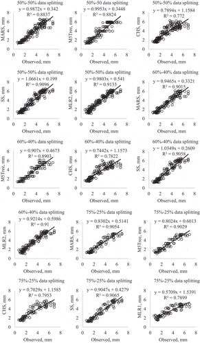
The error statistics of the MARS model for the Antakya station are given in the Appendix (Table A1). For this station also the MARS8 model had the best performance in estimating E_pan. The positive effect of the periodicity component on model accuracy is also clearly seen from the presented input combinations. The RMSE, MAE and NSE values of the MARS, M5Tree, CHS, SS and MLR methods are compared in Table A2. Here also the MARS method outperforms the M5Tree, CHS, SS and MLR methods with respect to three comparison criteria. The superior accuracy of SS over CHS and MLR is clearly seen from the average statistics. For Antakya station also, the accuracy of the methods was increased by the increase in training data length. The model accuracy fluctuated considerably with respect to different train-test strategies. From this, we can say that using only one data-splitting strategy may mislead the modeller; therefore, different splitting rules are needed to obtain more robust results. The regression trees of the optimal MARS and M5Tree models in the test phase under the 75%–25% train-test scenario for Antakya station are given in Tables A3 and A4.

For Merin station, the error statistics of the MARS models are presented in Table A5. Again, the MARS model with the eighth input combination (T_max, R_a and α) performed the best in all splitting strategies. For this station, including the periodicity component also increased the model accuracy in E_pan estimation. Table A6 compares the five models, again showing the superior accuracy of the MARS models. However, under the 75%–25% data-splitting scenario, the SS model provided better estimates than the MARS and M5Tree models. Here also an increment in training data generally had a positive effect on model accuracy in E_pan estimation. According to the average NSE statistics, the MARS, M5Tree and SS models gave very good estimates. Comparison of three stations shows that the model accuracy is lower in estimating E_pan for the Antakya station. The main reason for this could be the higher data range and lower correlation between the T_min/T_max/R_a and E_pan for this station. The regression trees of the optimal MARS and M5Tree models for Antakya station in the test phase, under the 75%–25% train-test scenario, are given in Tables A7 and A8.

The observed and estimated E_pan values obtained by each method in the test period are illustrated in Figure 4 for the Adana station. The figures for Antakya and Mersin stations are given in the Appendix (Figs A1 and A2, respectively). Only the best MLR models were included in the scatter plots. It should be noted that all the applied models provided good E_pan estimates using only temperature data, except for the CHS and MLR models, which had scattered E_pan values in most cases. The MARS models, comprising T_max, R_a and α inputs, generally had less scattered E_pan estimates compared to the other models. The SS model also had less scattered estimates than the CHS and MLR models.

Figure A1. Observed and estimated E_pan by the MARS, M5tree, CHS, SS and MLR methods in the test period – Antakya station.

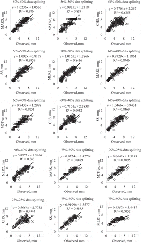
Figure A2. Observed and estimated E_pan by the MARS, M5tree, CHS, SS and MLR methods in the test period – Mersin station.

As mentioned before, Wang et al. (2017a) employed six different data-driven methods for modelling monthly E_pan of different climates in China. They obtained mean R² values for the temperature based on MLPNN, GRNN, FG, LSSVM, MARS and ANFIS models, using only temperature as input data, of 0.815, 0.809, 0.796, 0.788, 0.808 and 0.756, respectively. Wang et al. (2017c) estimated E_pan of six stations in China using three different data-driven methods and obtained mean R² values for the best temperature-based FG, ANFIS and M5Tree models of 0.835, 0.787 and 0.816, respectively. Malik et al. (2018) applied two different data-driven methods using maximum and minimum temperature (T_min and T_max), relative humidity, wind speed and sunshine hours as inputs. They obtained R² values for the best SOM and RBFNN models of 0.874 and 0.834, respectively. In this study, the mean R² values of the three stations are 0.873 and 0.825 for the best MARS and M5Tree models, respectively. This comparison suggests the usefulness of these heuristic regression methods in estimating monthly E_pan.

Conclusion

This study compared the accuracy of two heuristic regression methods, MARS and M5Tree, in estimating monthly E_pan using limited climatic data, minimum and maximum temperatures. The effect of periodicity (month of the year) on the accuracy of the models was also examined. The estimates of the heuristic methods were compared with those of the empirical CHS, SS and MLR methods. Data from three stations in Turkey were used by applying three train-test data-splitting strategies (50%–50%, 60%–40% and 75%–25%). The results may be summarized as follows:

• the MARS model generally had better accuracy than the M5Tree, CHS and SS models in estimating monthly E_pan using only temperature data;

• increasing the proportion of training to test data generally had a positive effect on the accuracy of the applied models;

• the estimation performance of the MARS and M5Tree models was increased by including a periodicity component as input;

• in the SS models, extraterrestrial radiation was successfully used instead of solar radiation and gave very satisfactory estimates;

• the SS model performed better than the CHS and MLR models for all three stations, which showed that the SS model could be used successfully for estimating E_pan with only minimum and maximum temperature data; and

• based on the application result, one splitting strategy is not recommended: model accuracy fluctuated considerably with respect to the different data-splitting strategies used; therefore, various data-splitting rules are required for better evaluation of the applied models in estimation of E_pan.

In this study, we tested the accuracy of two new heuristic approaches in estimating pan evaporation, E_pan, using data from three stations in Turkey. In future studies, other data-driven methods (e.g. support vector machine and extreme learning machine) may be tested using more data from other regions for comparison with this study.

Disclosure statement

No potential conflict of interest was reported by the authors.

Appendix

Table A1. Error statistics of various input combinations and data-splitting strategies – Antakya station. T_min, T_max, R_a and α are minimum and maximum temperatures, extraterrestrial radiation, and periodicity (month number), respectively. RMSE, MAE and NSE are root mean square error, mean absolute error and efficiency coefficient, respectively. Bold values indicate the best performance.

Model	Input	Training			Test
		RMSE (mm)	MAE (mm)	NSE	RMSE (mm)	MAE (mm)	NSE
50% training and 50% test
MARS1	Tmin	1.321	1.036	0.770	1.741	1.469	0.328
MARS2	Tmax	1.573	1.149	0.674	1.880	1.522	0.216
MARS3	Tmin, Ra	1.264	0.990	0.790	1.729	1.461	0.337
MARS4	Tmax, Ra	1.593	1.166	0.666	1.974	1.521	0.136
MARS5	Tmin, α	1.236	0.919	0.799	11.08	8.189	−26.2
MARS6	Tmax, α	1.230	0.925	0.801	1.438	1.254	0.541
MARS7	Tmin, Ra, α	1.193	0.889	0.812	1.582	1.322	0.445
MARS8	Tmax, Ra, α	1.234	0.926	0.799	1.400	1.223	0.565
MARS9	Tmin, Tmax, Ra	1.245	0.936	0.796	1.713	1.489	0.349
MARS10	Tmin, Tmax, Ra, α	1.210	0.910	0.807	1.563	1.321	0.869
60% training and 40% test
MARS1	Tmin	1.276	0.997	0.771	1.789	1.496	0.282
MARS2	Tmax	1.535	1.129	0.669	1.776	1.399	0.293
MARS3	Tmin, Ra	1.275	0.975	0.771	1.578	1.382	0.442
MARS4	Tmax, Ra	1.540	1.131	0.667	1.653	1.216	0.388
MARS5	Tmin, α	1.200	0.895	0.797	13.53	9.896	−40.0
MARS6	Tmax, α	1.187	0.883	0.802	1.344	1.167	0.595
MARS7	Tmin, Ra, α	1.186	0.884	0.802	1.445	1.240	0.532
MARS8	Tmax, Ra, α	1.189	0.888	0.801	1.317	1.157	0.611
MARS9	Tmin, Tmax, Ra	1.197	0.886	0.798	1.673	1.452	0.854
MARS10	Tmin, Tmax, Ra, α	1.224	0.926	0.789	1.507	1.307	0.848
75% training and 25% test
MARS1	Tmin	1.294	1.011	0.753	1.634	1.394	0.336
MARS2	Tmax	1.541	1.123	0.649	1.651	1.272	0.322
MARS3	Tmin, Ra	1.270	0.960	0.761	1.469	1.309	0.464
MARS4	Tmax, Ra	1.541	1.123	0.649	1.471	1.054	0.462
MARS5	Tmin, α	1.198	0.892	0.788	12.20	9.700	−36.0
MARS6	Tmax, α	1.197	0.891	0.788	1.149	0.983	0.672
MARS7	Tmin, Ra, α	1.170	0.881	0.798	1.293	1.122	0.584
MARS8	Tmax, Ra, α	1.193	0.892	0.790	1.106	0.947	0.696
MARS9	Tmin, Tmax, Ra	1.229	0.917	0.777	1.472	1.305	0.831
MARS10	Tmin, Tmax, Ra, α	1.182	0.875	0.794	1.353	1.190	0.831
Average
MARS1	Tmin	1.297	1.015	0.765	1.721	1.453	0.315
MARS2	Tmax	1.550	1.134	0.664	1.769	1.398	0.277
MARS3	Tmin, Ra	1.270	0.975	0.774	1.592	1.384	0.414
MARS4	Tmax, Ra	1.558	1.140	0.661	1.699	1.264	0.329
MARS5	Tmin, α	1.211	0.902	0.795	12.27	9.262	−34.07
MARS6	Tmax, α	1.205	0.900	0.797	1.310	1.135	0.603
MARS7	Tmin, Ra, α	1.183	0.885	0.804	1.440	1.228	0.520
MARS8	Tmax, Ra, α	1.205	0.902	0.797	1.274	1.109	0.624
MARS9	Tmin, Tmax, Ra	1.224	0.913	0.790	1.619	1.415	0.678
MARS10	Tmin, Tmax, Ra, α	1.205	0.904	0.797	1.474	1.273	0.849

Table A2. Error statistics of each model for different data splitting strategies – Antakya station. See Table A1 for explanation of abbreviations and variables.

Model	Input	Training			Test
		RMSE (mm)	MAE (mm)	NSE	RMSE (mm)	MAE (mm)	NSE
50% training and 50% test
MARS	Tmax, Ra, α	1.234	0.926	0.799	1.400	1.223	0.565
M5Tree	Tmax, Ra, α	1.203	0.859	0.810	1.512	1.293	0.493
CHS	Tmin, Tmax, Ra	1.750	1.267	0.597	1.794	1.508	0.328
SS	Tmin, Tmax, Ra	1.422	1.083	0.734	1.599	1.327	0.466
MLR1	Tmax, Ra, α	1.784	1.418	0.581	1.679	1.433	0.375
MLR2	Tmin, Tmax, Ra	1.324	1.025	0.769	1.650	1.455	0.397
60% training and 40% test
MARS	Tmax, Ra, α	1.189	0.888	0.801	1.317	1.157	0.611
M5Tree	Tmax, Ra, α	1.095	0.800	0.831	1.390	1.181	0.567
CHS	Tmin, Tmax, Ra	1.695	1.226	0.596	1.715	1.467	0.361
SS	Tmin, Tmax, Ra	1.382	1.047	0.731	1.495	1.047	0.515
MLR1	Tmax, Ra, α	1.727	1.356	0.580	1.600	1.362	0.426
MLR2	Tmin, Tmax, Ra	1.287	0.996	0.767	1.571	1.396	0.447
75% training and 25% test
MARS	Tmax, Ra, α	1.193	0.892	0.790	1.106	0.947	0.696
M5Tree	Tmax, Ra, α	1.125	0.810	0.813	1.214	1.033	0.633
CHS	Tmin, Tmax, Ra	1.681	1.222	0.583	1.555	1.339	0.409
SS	Tmin, Tmax, Ra	1.372	1.015	0.722	1.297	1.120	0.589
MLR1	Tmax, Ra, α	1.707	1.343	0.569	1.398	1.159	0.514
MLR2	Tmin, Tmax, Ra	1.284	0.983	0.756	1.431	1.290	0.491
Average
MARS	Tmax, Ra, α	1.205	0.902	0.797	1.274	1.109	0.624
M5Tree	Tmax, Ra, α	1.141	0.823	0.818	1.372	1.169	0.564
CHS	Tmin, Tmax, Ra	1.709	1.238	0.592	1.688	1.438	0.366
SS	Tmin, Tmax, Ra	1.392	1.048	0.729	1.464	1.165	0.523
MLR1	Tmax, Ra, α	1.739	1.372	0.577	1.559	1.318	0.438
MLR2	Tmin, Tmax, Ra	1.298	1.001	0.764	1.551	1.380	0.445

Table A3. Regression tree of the MARS model in the test phase under the 75%–25% train-test scenario – Antakya station.

if (x1 <= 6.5) then f1_1 = 0	if (27 < x3 < 39) then begin
if (6.5 < x1 < 10) then begin	f3_1 = 0.1250*(x3–(39))^2 + 0.0046*(x3–(39))^3
f1_1 = 0.2041*(x1–(6.5))^2 – 0.0117*(x1–(6.5))^3	end
end	if (x3 >= (39)) then f3_1 = 0
if (x1 >= (10)) then f1_1 = x1 – (8)	BF3 = f3_1
BF1 = f1_1	if (x1 <= 3) then f4_1 = 0
if (x3 <= 27) then f2_1 = 0	if (3 < x1 < 6.5) then begin
if (27 < x3 < 39) then begin	f4_1 = 0.0816*(x1–(3))^2 0.0117*(x1–(3))^3
f2_1 –0.0417*(x3–(27))^2 + 0.0046*(x3–(27))^3	end
end	if (x1 >= (6.5)) then f4_1 = x1 – (5)
if (x3 >= (39)) then f2_1 = x3 – (37)	BF4 = f4_1
BF2 = f2_1
if (x3 <= 27) then f3_1 = –(x3 – (37))

y = 4.4 − 2.7*BF1 + 0.24*BF2 − 0.14*BF3 + 1.5*BF4

Table A4. Regression tree of the M5Tree model in the test phase under the 75%–25% train-test scenario – Antakya station.

if x2 <= 30.05	y = 3.38 (5)	y = 6.23636363636364 (11)
if x2 <= 22.2	else	else
if x3 <= 18.065	if x3 <= 30.07	y = –26.8422842763249 + 0.846253754363277*x2 (8)
y = 1.64259259259259 (54)	if x2 <= 35.45	else
else	if x3 <= 24.385	if x1 <= 8.5
y = 2.29375 (32)	y = 4.175 (8)	if x1 <= 6.5
else	else	y = 7.23870967741936 (31)
if x3 <= 32.215	y = 14.1182633066862 – 0.374156919854213*x3 (18)	else
if x2 <= 25.35	else	if x2 <= 36.9
y = 3.08571428571429 (28)	y = 4.35 (8)	y = 8.33265306122449 (49)
else	else	else
if x2 <= 25.9	if x1 <= 5.5	if x3 <= 37.165
y = 2.73333333333333 (12)	if x2 <= 33.55	y = 6.62 (5)
else	y = 4.61 (20)	else
if x2 <= 27.05	else	y = –5.0361905946748 + 0.309156506593668*x2 (9)
y = 3.35555555555556 (9)	if x3 <= 39.825	else
else	y = 5.3625 (8)	if x2 <= 39.25
y = 2.6625 (8)	else	y = 7.03461538461538 (26)
else	if x2 <= 36.2	else
if x3 <= 35.5		y = 5.91666666666667 (6)
y = 4.3 (10)
else

Table A5. Error statistics of various input combinations and data-splitting strategies – Mersin station. See Table A1 for explanation of abbreviations and variables. Bold values indicate the best performance.

Model	Input	Training			Test
		RMSE (mm)	MAE (mm)	NSE	RMSE (mm)	MAE (mm)	NSE
50% training and 50% test
MARS1	Tmin	0.971	0.780	0.722	0.876	0.686	0.692
MARS2	Tmax	1.078	0.819	0.658	1.008	0.780	0.592
MARS3	Tmin, Ra	0.839	0.660	0.793	0.642	0.518	0.835
MARS4	Tmax, Ra	1.127	0.854	0.626	0.905	0.705	0.671
MARS5	Tmin, α	0818	0.636	0.803	6.708	5.165	−17.0
MARS6	Tmax, α	0.781	0.612	0.820	0.638	0.507	0.837
MARS7	Tmin, Ra, α	0.772	0.592	0.825	0.566	0.438	0.872
MARS8	Tmax, Ra, α	0.758	0.591	0.831	0.640	0.493	0.835
MARS9	Tmin, Tmax, Ra	0.833	0.655	0.796	0.720	0.557	0.792
MARS10	Tmin, Tmax, Ra, α	0.747	0.571	0.836	0.673	0.507	0.818
60% training and 40% test
MARS1	Tmin	0.951	0.750	0.716	0.752	0.598	0.787
MARS2	Tmax	1.077	0.813	0.636	0.943	0.717	0.665
MARS3	Tmin, Ra	0.808	0.619	0.795	0.626	0.482	0.852
MARS4	Tmax, Ra	1.085	0.818	0.630	0.851	0.697	0.727
MARS5	Tmin, α	0.777	0.601	0.810	9.294	6.742	−31.6
MARS6	Tmax, α	0.758	0.576	0.820	0.573	0.461	0.876
MARS7	Tmin, Ra, α	0.735	0.557	0.830	0.585	0.424	0.871
MARS8	Tmax, Ra, α	0.737	0.555	0.830	0.540	0.417	0.890
MARS9	Tmin, Tmax, Ra	0.773	0.583	0.812	0.659	0.499	0.836
MARS10	Tmin, Tmax, Ra, α	0.727	0.552	0.834	0.611	0.439	0.859
75% training and 25% test
MARS1	Tmin	0.873	0.670	0.744	0.855	0.673	0.759
MARS2	Tmax	1.026	0.763	0.646	1.005	0.792	0.667
MARS3	Tmin, Ra	0.757	0.566	0.807	0.604	0.479	0.880
MARS4	Tmax, Ra	1.054	0.787	0.627	0.859	0.691	0.757
MARS5	Tmin, α	0.717	0.532	0.827	5.404	4.262	−8.62
MARS6	Tmax, α	0.686	0.503	0.842	0.536	0.384	0.905
MARS7	Tmin, Ra, α	0.681	0.502	0.844	0.620	0.460	0.873
MARS8	Tmax, Ra, α	0.699	0.516	0.836	0.557	0.402	0.898
MARS9	Tmin, Tmax, Ra	0.729	0.541	0.822	0.673	0.500	0.851
MARS10	Tmin, Tmax, Ra, α	0.675	0.500	0.847	0.594	0.429	0.884
Average
MARS1	Tmin	0.932	0.733	0.727	0.828	0.652	0.746
MARS2	Tmax	1.060	0.798	0.647	0.985	0.763	0.641
MARS3	Tmin, Ra	0.801	0.615	0.798	0.624	0.493	0.856
MARS4	Tmax, Ra	1.089	0.820	0.628	0.872	0.698	0.718
MARS5	Tmin, α	273	0.590	0.813	7.135	5.390	−19.07
MARS6	Tmax, α	0.742	0.564	0.827	0.582	0.451	0.873
MARS7	Tmin, Ra, α	0.729	0.550	0.833	0.590	0.441	0.872
MARS8	Tmax, Ra, α	0.731	0.554	0.832	0.579	0.437	0.874
MARS9	Tmin, Tmax, Ra	0.778	0.593	0.810	0.684	0.519	0.826
MARS10	Tmin, Tmax, Ra, α	0.716	0.541	0.839	0.626	0.458	0.854

Table A6. Error statistics of each model for different data-splitting strategies – Mersin station. See Table A1 for explanation of abbreviations and variables.

Model	Input	Training			Test
		RMSE (mm)	MAE (mm)	NSE	RMSE (mm)	MAE (mm)	NSE
50% training and 50% test
MARS	Tmax, Ra, α	0.758	0.591	0.831	0.640	0.493	0.835
M5Tree	Tmax, Ra, α	0.731	0.533	0.843	0.661	0.518	0.825
CHS	Tmin, Tmax, Ra	1.202	0.890	0.575	0.889	0.704	0.703
SS	Tmin, Tmax, Ra	0.933	0.712	0.744	0.682	0.535	0.825
MLR1	Tmax, Ra, α	1.117	0.905	0.633	0.857	0.711	0.705
MLR2	Tmin, Tmax, Ra	0.902	0.716	0.761	0.675	0.583	0.817
60% training and 40% test
MARS	Tmax, Ra, α	0.737	0.555	0.830	0.540	0.417	0.890
M5Tree	Tmax, Ra, α	0.692	0.516	0.849	0.563	0.429	0.880
CHS	Tmin, Tmax, Ra	1.158	0.850	0.579	0.824	0.646	0.751
SS	Tmin, Tmax, Ra	0.904	0.693	0.743	0.664	0.518	0.838
MLR1	Tmax, Ra, α	1.067	0.840	0.642	0.846	0.703	0.730
MLR2	Tmin, Tmax, Ra	0.865	0.681	0.765	0.594	0.497	0.867
75% training and 25% test
MARS	Tmax, Ra, α	0.699	0.516	0.836	0.557	0.402	0.898
M5Tree	Tmax, Ra, α	0.636	0.444	0.864	0.578	0.432	0.890
CHS	Tmin, Tmax, Ra	1.096	0.790	0.596	0.823	0.648	0.778
SS	Tmin, Tmax, Ra	0.848	0.630	0.758	0.543	0.421	0.903
MLR1	Tmax, Ra, α	1.009	0.783	0.658	0.911	0.760	0.727
MLR2	Tmin, Tmax, Ra	1.284	0.983	0.756	1.431	1.290	0.491
Average
MARS	Tmax, Ra, α	0.731	0.554	0.832	0.579	0.437	0.874
M5Tree	Tmax, Ra, α	0.686	0.498	0.852	0.601	0.460	0.865
CHS	Tmin, Tmax, Ra	1.152	0.843	0.583	0.845	0.666	0.744
SS	Tmin, Tmax, Ra	0.895	0.678	0.748	0.630	0.491	0.855
MLR1	Tmax, Ra, α	1.064	0.843	0.644	0.871	0.725	0.721
MLR2	Tmin, Tmax, Ra	1.017	0.793	0.761	0.900	0.790	0.725

Table A7. Regression tree of the MARS model in the test phase under the 75%–25% train-test scenario – Mersin station.

if (x1 <= 4) then f1_1 = 0	if (x2 >= (32)) then f5_1 = x2 – (31)
if (4 < x1 < 7.5) then begin	BF5 = f5_1
f1_1 = –0.1633*(x1–(4))^2+ 0.0583*(x1–(4))^3	if (x2 <= 32) then f6_1 = 0
end	if (32 < x2 < 36) then begin
if (x1 >= (7.5)) then f1_1 = x1 – (7)	f6_1 = 0.3125*(x2–(32))^2 – 0.0313*(x2–(32))^3
BF1 = f1_1	end
if (x1 <= 7.5) then f2_1 = –(x1 – (8))	if (x2 >= (36)) then f6_1 = x2 – (33)
if (7.5 < x1 < 8.5) then begin	BF6 = f6_1
f2_1 = 0.5*(x1–(8.5))^2	if (x2 <= 31) then f7_1 = –(x2 – (31))
end	if (31 < x2 < 31) then begin
if (x1 >= (8.5)) then f2_1 = 0	p7_1 = (3*(31) – 2*(31) – (31)) / ((31) – (31))^2
BF2 = f2_1	r7_1 = ((31) + (31) - 2*(31)) / ((31) - (31))^3
if (x3 <= 17) then f3_1 = –(x3 – (18))	f7_1 = p7_1*(x2-(31))^2 + r7_1*(x2-(31))^3
if (17 < x3 < 30) then begin	end
f3_1 = –0.0592*(x3–(30))^2 – 0.005*(x3–(30))^3	if (x2 >= (31)) then f7_1 = 0
end	BF7 = f7_1
if (x3 >= (30)) then f3_1 = 0	if (x2 <= 23) then f8_1 = –(x2 – (30))
BF3 = f3_1	if (23 < x2 < 30) then begin
if (x1 <= 8.5) then f4_1 = 0	f8_1 = 0.2857*(x2–(30))^2 + 0.0204*(x2–(30))^3
if (8.5 < x1 < 11) then begin	end
f4_1 = 0.56*(x1–(8.5))^2 – 0.096*(x1–(8.5))^3	if (x2 >= (30)) then f8_1 = 0
end	BF8 = f8_1
if (x1 >= (11)) then f4_1 = x1 – (9)	if (x2 <= 30) then f9_1 = 0
BF4 = f4_1	if (30 < x2 < 31) then begin
if (x2 <= 31) then f5_1 = 0	f9_1 = 2*(x2–(30))^2 – (x2–(30))^3
if (31 < x2 < 32) then begin	end
f5_1 = 2*(x2–(31))^2 – (x2–(31))^3	if (x2 >= (31)) then f9_1 = x2 – (30)
end	BF9 = f9_1

y = 6.1 − 0.88*BF1 − 0.83*BF2 + 0.22*BF3 − 0.53*BF4 − 1.5*BF5 + 0.58*BF6 + 0.27*BF7 − 0.22*BF8 + 1.1*BF9

Table A8. Regression tree of the M5Tree model in the test phase under the 75%–25% train-test scenario – Mersin station.

if x3 <= 29.95	if x1 <= 6.5	if x1 <= 5.5
if x3 <= 23.04	if x2 <= 22.25	y = –0.200432900432907 + 0.884632034632036*x1 (43)
if x3 <= 17.735	y = 2.78 (5)
if x2 <= 21.85	else	else
y = 1.38529411764706 (34)	if x2 <= 24	if x3 <= 31.245
else	y = 2.08 (5)	y = 4.69411764705882 (17)
y = 4.69700301854218 – 0.134756360500203*x2 (8)	else	else
else	if x2 <= 26.5	if x1 <= 6.5
if x2 <= 22.75	y = 2.81666666666667 (6)	if x2 <= 32.3
if x2 <= 19.25	else	if x2 <= 31.25
y = 1.92 (5)	y = 2.26 (5)	if x2 <= 30.1
else	else	y = 5.48 (5)
if x2 <= 20.2	if x2 <= 31.65	else
y = 1.5 (4)	if x2 <= 30.9	y = 4.41666666666667 (6)
else	y = 3.35 (6)	else
y = 1.64444444444444 (9)	else	y = 6.075 (4)
else	y = 4.24 (5)	else
if x2 <= 27	else	y = 5.025 (8)
if x2 <= 25.3	if x2 <= 33.25	else
y = 2.2 (7)	y = 2.625 (4)	if x2 <= 31.85
else	else	y = 6.62222222222222 (9)
y = 1.77142857142857 (7)	y = 3.28571428571429 (7)	else
else	else	if x2 <= 32.95
y = 2.24 (10)		y = 5.70666666666667 (15)
else		else
		y = 5.288 (25)

References

- Abraham, A., Steinberg, D., and Philip, N.S., 2001. Rainfall forecasting using soft computing models and multivariate adaptive regression splines. IEEE Transactions on Systems, Man, and Cybernetics: Special Issue on Fusion of Soft Computing and Hard Computing in Industrial Applications, 1, 1–6.
- Adamala, S., Raghuwanshi, N.S., and Mishra, A., 2018. Development of generalized higher-order neural network-based models for estimating pan evaporation. In: V. Singh, S. Yadav, and R. Yadava, eds. Hydrologic modeling. Water science and technology library. Vol. 81, Singapore: Springer. 55–71. doi:10.1007/978-981-10-5801-1_5
- AL-Musaylh, M.S., et al., 2018. Two-phase particle swarm optimized-support vector regression hybrid model integrated with improved empirical mode decomposition with adaptive noise for multiple-horizon electricity demand forecasting. Applied Energy, 217, 422–439. doi:10.1016/j.apenergy.2018.02.140
- Al-Shalan, A. and Salih, A.M.A., 1987. Evaporation estimation in extremely arid areas. Journal of Irrigation and Drainage Engineering, 113, 565–574. doi:10.1061/(ASCE)0733-9437
- Arunkumar, R., Jothiprakash, V., and Sharma, K.J., 2017. Artificial intelligence techniques for predicting and mapping daily pan evaporation. Journal of the Institution of Engineers (India): Series A, 98 (3), 219–231. doi:10.1007/s40030-017-0215-1
- Cahoon, J.E., Costello, T.A., and Ferguson, J.A., 1991. Estimating pan evaporation using limited meteorological observations. Agricultural and Forest Meteorology, 55, 181–190. doi:10.1016/0168-1923(91)90061-T
- Chu, C.R., et al., 2010. A wind tunnel experiment on the evaporation rate of Class A evaporation pan. Journal of Hydrology, 381, 221–224. doi:10.1016/j.jhydrol.2011.10.043
- Deo, R.C., Kisi, O., and Singh, V.P., 2017. Drought forecasting in eastern Australia using multivariate adaptive regression spline, least square support vector machine and M5Tree model. Atmospheric Research, 184, 149–175. doi:10.1016/j.atmosres.2016.10.004
- Deo, R.C. and Samui, P., 2017. Forecasting evaporative loss by least-square support-vector regression and evaluation with genetic programming, Gaussian process, and minimax probability machine regression: case study of Brisbane city. ASCE Journal of Hydrologic Engineering, 22 (6), 05017003. doi:10.1061/(ASCE)HE.1943-5584.0001506
- Eray, O., Mert, C., and Kisi, O., 2017. Comparison of multi-gene genetic programming and dynamic evolving neural-fuzzy inference system in modeling pan evaporation. Hydrology Research. doi:10.2166/nh.2017.076
- Friedman, J.H., 1991. Multivariate adaptive regression splines. The Annals of Statistics, 19 (1), 1–67. doi:10.1214/aos/1176347963
- Ghasemzadeh, A. and Ahmed, M.M., 2018. Utilizing naturalistic driving data for in-depth analysis of driver lane-keeping behavior in rain: non-parametric MARS and parametric logistic regression modeling approaches. Transportation Research Part C, 90, 379–392. doi:10.1016/j.trc.2018.03.018
- Ghiasi, R., Ghasemi, M.R., and Noori, M., 2018. Comparative studies of metamodeling and AI-Based techniques in damage detection of structures. Advances in Engineering Software, 125, 101–112. doi:10.1016/j.advengsoft.2018.02.006
- Ghorbani, M.A., et al., 2017. Pan evaporation prediction using a hybrid multilayer perceptron-firefly algorithm (MLP-FFA) model: case study in North Iran. Theoretical and Applied Climatology. doi:10.1007/s00704-017-2244-0
- Goyal, M.K., et al., 2014. Modeling of daily pan evaporation in sub-tropical climates using ANN, LS-SVR, Fuzzy logic, and ANFIS. Expert Systems with Applications, 41, 5267–5276. doi:10.1016/j.eswa.2014.02.047
- Hamze-Ziabari, S.M. and Bakhshpoori, T., 2018. Improving the prediction of ground motion parameters based on an efficient bagging ensemble model of M5` and CART algorithms. Applied Soft Computing, 68, 147–161. doi:10.1016/j.asoc.2018.03.052
- Hargreaves, G.H. and Samani, Z.A., 1982. Estimating potential evapotranspiration. Journal of Irrigation and Drainage Engineering (ASCE), 108 (IR3), 223–230.
- Hargreaves, G.H. and Samani, Z.A., 1985. Reference crop evapotranspiration from temperature. Transaction of ASAE, 1 (2), 96–99.
- Jekabsons, G. (2016a). ARESLab adaptive regression splines toolbox for Matlab/Octave ver. 1.13.0. Institute of Applied Computer Systems Riga Technical University, Latvia. Available from: http://www.cs.rtu.lv/jekabsons/Files/ARESLab.pdf
- Jekabsons, G. (2016b). M5PrimeLab: M5ʹ Regression Tree and Model Tree ensemble toolbox for Matlab/Octave ver. 1.7.0. Institute of Applied Computer Systems Riga Technical University, Latvia. Available from: http://www.cs.rtu.lv/jekabsons/Files/M5PrimeLab.pdf.
- Keshtegar, B. and Kisi, O., 2016. A nonlinear modelling-based high-order response surface method for predicting monthly pan evaporation. Hydrology and Earth System Sciences Discussion. doi:10.5194/hess-2016-191
- Keshtegar, B. and Kisi, O., 2017. Modified response-surface method: new approach for modeling pan evaporation. Journal of Hydrologic Engineering ASCE, 22 (10), 04017045. doi:10.1061/(ASCE).HE.1943-5584.0001541
- Kim, S. and Kim, H.S., 2008. Neural networks and genetic algorithm approach for nonlinear evaporation and evapotranspiration modeling. Journal of Hydrology, 351 (3–4), 299–317. doi:10.1016/j.jhydrol.2007.12.014
- Kim, S., Shiri, J., and Kisi, O., 2012. Pan evaporation modeling using neural computing approach for different climatic zones. Water Resources Management, 26, 3231–3249. doi:10.1007/s11269-012-0069-2
- Kisi, O., et al., 2016. Daily pan evaporation modeling using chi-squared automatic interaction detector, neural networks, classification and regression tree. Computers and Electronics in Agriculture, 122, 112–117. doi:10.1016/j.compag.2016.01.026
- Li, Y., et al., 2018. Learning deep generative models of graphs. arXiv:1803.03324. Available from: https://arxiv.org/pdf/1803.03324.pdf
- Lokuge, W., et al., 2018. Design of fly ash geopolymer concrete mix proportions using multivariate adaptive regression spline model. Construction and Building Materials, 166, 472–481. doi:10.1016/j.conbuildmat.2018.01.175
- Malik, A., Kumar, A., and Kisi, O., 2017. Monthly pan-evaporation estimation in Indian central Himalayas using different heuristic approaches and climate based models. Computers and Electronics in Agriculture, 143, 302–313. doi:10.1016/j.compag.2017.11.008
- Malik, A., Kumar, A., and Kisi, O., 2018. Daily pan-evaporation estimation using heuristic methods with gamma test. Journal of Irrigation and Drainage Engineering ASCE, 144 (9), 04018023. doi:10.1061/(ASCE)IR.1943-4774.0001336
- Mehdizadeh, S., 2018. Assessing the potential of data-driven models for estimation of long-term monthly temperatures. Computers and Electronics in Agriculture, 144, 114–125. doi:10.1016/j.compag.2017.11.038
- Moriasi, D.N., et al., 2007. Model evaluation guidelines for systematic quantification of accuracy in watershed simulations. Transactions of the American Society of Agricultural and Biological Engineers, 50, 885–900. doi:10.13031/2013.23153
- Ozmen, A., Yılmaz, Y., and Weber, G.W., 2018. Natural gas consumption forecast with MARS and CMARS models for residential users. Energy Economics, 70, 357–381. doi:10.1016/j.eneco.2018.01.022
- Pammar, L. and Deka, P.C., 2017. Daily pan evaporation modeling in climatically contrasting zones with hybridization of wavelet transforms and support vector machines. Paddy and Water Environment, 15, 711–722. doi:10.1007/s10333-016-0571-x
- Quinlan, J.R. (1992). Learning with continuous classes. In: Proceedings of the Fifth Australian Joint Conference on Artificial Intelligence (Hobart, Australia, 16-18 November). Singapore: World Scientific, 343–348.
- Rahimikhoob, A., 2009. Estimating daily pan evaporation using artificial neural network in a semi-arid environment. Theoretical and Applied Climatology, 98, 101–105. doi:10.1007/s00704-008-0096-3
- Ranjbar, A. and Mahjouri, N., 2018. Development of an efficient surrogate model based on aquifer dimensions to prevent seawater intrusion in anisotropic coastal aquifers, case study: the Qom aquifer in Iran. Environmental Earth Sciences, 77, 418. doi:10.1007/s12665-018-7592-2
- Sanikhani, H., et al., 2018. Non-tuned data intelligent model for soil temperature estimation: a new approach. Geoderma, 330, 52–64. doi:10.1016/j.geoderma.2018.05.030
- Sensoy, S., Demircan, M., and Ulupinar, Y. (2016). Climate of Turkey, Turkish State Meteorological Service, Ankara, Turkey. https://www.researchgate.net/publication/296597022_Climate_of_Turkey.
- Shiri, J., et al., 2011. Estimating daily pan evaporation from climatic data of the State of Illinois, USA using adaptive neuro-fuzzy inference system (ANFIS) and artificial neural network (ANN). Hydrology Research, 42 (6), 491–502. doi:10.2166/nh.2011.020
- Shiri, J., Marti, P., and Singh, V.P., 2014. Evaluation of gene expression programming approaches for estimating daily evaporation through spatial and temporal data scanning. Hydrological Processes, 28, 1215–1225. doi:10.1002/hyp.9669
- Stephens, J.C. and Stewart, E.H., 1963. A comparison of procedures for computing evaporation and evapotranspiration. General Assembly of Berkeley, 123–133: IAHS Publ. no. 62.
- Wang, L., et al., 2017a. Pan Evaporation modeling using six different heuristic computing methods in different climates of China. Journal of Hydrology, 544, 407–427. doi:10.1016/j.jhydrol.2016.11.059
- Wang, L., et al., 2017b. Pan evaporation modeling using four different heuristic approaches. Computers and Electronics in Agriculture, 140, 203–213. doi:10.1016/j.compag.2017.05.036
- Wang, L., et al., 2017c. Evaporation modelling using different machine learning techniques. International Journal of Climatology, 37 (S1), 1076–1092. doi:10.1002/joc.5064
- Wang, Y. and Witten, I.H., 1997. Induction of model trees for predicting continuous lasses. In: Proceedings of the Poster Papers of the European Conference on Machine Learning. Prague: University of Economics, Faculty of Informatics and Statistics. doi:10.1007/s11269-013-0440-y
- Wurbs, R.A. and Ayala, R.A., 2014. Reservoir evaporation in Texas, USA. Journal of Hydrology, 510, 1–9. doi:10.1016/j.jhydrol.2013.12.011
- Yilmaz, B., et al., 2018. Estimating suspended sediment load with multivariate adaptive regression spline, teaching learning based optimization, and artificial bee colony models. Science of the Total Environment, 639, 826–840. doi:10.1016/j.scitotenv.2018.05.153