The influence of dependence in characterizing multi-variable uncertainty for climate change impact assessments

ABSTRACT

Few approaches exist that explicitly use the uncertainty associated with the spread of climate model simulations in assessing climate change impacts. An approach that does so is second-order approximation (SOA). This incorporates quantification of uncertainty to ascertain its impact on the derived response using a Taylor series expansion of the model. This study uses SOA in a statistical downscaling model of monthly streamflow, with a focus on the influence of dependence in the uncertainty of multiple atmospheric variables. Uncertainty is quantified using the square root error variance concept with a new extension that allows the inter-dependence terms among the atmospheric variable uncertainty to be specified. Applying the model to selected point locations in Australia, it is noted that the downscaling results differ considerably from downscaling that ignores uncertainty. However, when the effects of dependence in uncertainty are incorporated, the results differ according to the regional variations in dependence structure.

KEYWORDS:

• statistical downscaling
• uncertainty
• climate variable uncertainty dependence
• Taylor series

Editor R. Woods Associate editor A. Langousis

1 Introduction

The range of general circulation models (GCMs) and simulations for multiple representative concentration pathways (RCPs) (Van Vuuren et al. 2011) now available are some of the causes of uncertainty in climate change assessments (Tebaldi and Knutti 2007). Eghdamirad et al. (2017) proposed a framework to incorporate this uncertainty in climate change impact assessments, using downscaling of monthly streamflow to point locations to illustrate the framework. The framework was based on second-order approximation (SOA) of the Taylor series expansion (Benjamin and Cornell 1970) of the adopted statistical downscaling model. It was shown that ignoring the uncertainty of atmospheric predictors in downscaling results in biases in future projections of streamflow, particularly in low flows (Eghdamirad et al. 2017). This specific bias is introduced because of the nonlinear nature of the relationship between atmospheric variables and streamflow in the downscaling model, and is magnified when the extent of uncertainty associated with the atmospheric variables is large.

The SOA framework used by Eghdamirad et al. (2017) assumed that the uncertainty in each of the climate variables was independent of the other variables. However, given the dynamic nature of the climate system, this assumption should be questioned, as highly correlated atmospheric variables are expected to exhibit equivalently high correlations in their associated uncertainty (Bergant and Kajfež-Bogataj 2005, Fowler et al. 2007, 2016). The uncertainty of climate variables has been used to assess the accuracy of GCMs in modelling climatic variables (Hawkins et al. 2015). Braunisch et al. (2013) showed that using correlated climate variables in climate change impact assessment is a major source of uncertainty. A question that has not yet been addressed is how cross-correlation of uncertainties in climate variables should be quantified? Furthermore, what is the influence of this correlation of uncertainties on impact assessments of climate change? This research aims, for the first time, to investigate and quantify the extent of this dependence between the uncertainty of different variables and extend the SOA framework to use both the uncertainty and its cross-variable dependence for statistical downscaling of streamflow. Finally, the spatial patterns of climate variability uncertainty and its dependence are presented to suggest regions of the world where the extended SOA framework will be most useful.

Uncertainty in climate projections can be quantified using the square root of error variance (SREV). The SREV was introduced by Woldemeskel et al. (2012) for Coupled Model Intercomparison Project Phase 3 (CMIP3) rainfall and temperature, and extended to CMIP5 rainfall and temperature (Woldemeskel et al. 2016). Eghdamirad et al. (2016) used the SREV to investigate the uncertainty of upper air climate variables. The SREV assumes that uncertainty in climatic model simulations can be described by considering the spread of an ensemble of model projections (Hawkins and Sutton 2009, 2010, Yip et al. 2011). However, the dependence of this uncertainty has rarely been considered in previous work on climate model convergence. To achieve this, an extension of the SREV is proposed here that can account for the dependence between the uncertainties of different climate variables.

Section 2 presents the rationale behind SOA and an extension to include uncertainty dependence along with details of the uncertainty metric proposed. Section 3 presents an example of the new framework applied to a streamflow downscaling case study and discusses the results. Conclusions are presented in Section 4.

2 Methodology

2.1 SOA incorporating dependence

Second-order approximation (SOA) is an uncertainty analysis method introduced by Benjamin and Cornell (1970) that is based on the second-order expansion of the Taylor series. Its basis is the well-known logic that biases can result from assuming that the average of a function is equivalent to the use of the same function using an averaged input. The extent of bias depends on the nonlinearity of the process that forms the basis of the SOA. The approximation calculates the mean and variance of a function using the mean and variance of the input variables along with a second derivative of the adopted model (Haan 2002). Examples of SOA applications include groundwater flow (Dettinger and Wilson 1981, Panda et al. 2008, Wang and Hsu 2009), water quality (Xue et al. 2010), geographic information systems (Xue et al. 2015), and hydraulic analyses (Alvisi and Franchini 2010).

Benjamin and Cornell (1970) showed that by considering the function f:

(1) $Y=f\left(X_1,X_2,...,X_n\right)$(1)

a second-order Taylor series approximation of f to the expected value of Y can be written as follows:

(2) $E\left(Y\right)\approx f\left(m_{X_1},m_{X_2},...,m_{X_n}\right)+\frac{1}{2}\sum _{i=1}^n\sum _{j=1}^n{\left.\frac{{\mathrm{\partial }}^{2}f}{\mathrm{\partial }{x}_i\mathrm{\partial }{x}_j}\right|}_m\mathrm{c}\mathrm{o}\mathrm{v}\left[X_i,X_j\right]$(2)

in which $(X_1,X_2,...,X_n)$ are the n input variables, $\left(m_{X_1},m_{X_2},...,m_{X_n}\right)$are their respective expected values, and ${\mathrm{\partial }}^{2}f/\mathrm{\partial }{x}_i\mathrm{\partial }{x}_j{|}_m$is the pairwise second partial derivative of $f\left(x_1,x_2,...,x_n\right)$ with respect to variables x_i and x_j at time step i evaluated at their expected means. If the input variables are independent then the second term of the SOA collapses to only consider the variance of each input as used by Eghdamirad et al. (2017). This error variance is denoted EV in the remainder of this paper ($\mathrm{E}\mathrm{V}=\mathrm{S}\mathrm{R}\mathrm{E}{\mathrm{V}}^2$for each variable, percentile, and model considered). The impact of considering the interdependence terms in the covariance detailed in Equation (2) had not been attempted in hydro-climatic modelling prior to this study.

2.2 Uncertainty of climate variables and their dependence

Eghdamirad et al. (2016, 2017) quantified and incorporated the uncertainty of climate variables into downscaling. To expand this previous framework, bivariate or multivariate uncertainty needs to be quantified. The EV has previously been developed to express climate variable uncertainty, estimated as a measure of variability across alternative model simulations for each percentile of interest. Here, EV is extended to also include the interactions among different climate variables and is termed error variance dependence (EVd). A brief summary of the rationale behind EV is presented in the following text, which is then followed by a derivation of the extended version of the metric.

When considering the uncertainty or spread of GCM simulations, the primary difficulty to overcome is how to group the simulations, as time correspondence among alternative models cannot be assumed. Woldemeskel et al. (2012) suggested that the cumulative distribution function (cdf) of simulations could be compared instead of their time series to estimate the spread of the model simulations for each percentile of interest. For each climate variable, the projected values were sorted and the values at the same rank from each model were grouped. The standard deviation of this group of values was termed the SREV and used to represent the uncertainty for each associated rank or percentile. Transferring this uncertainty from rank space to the original time space, a corresponding time series of uncertainty was generated for each GCM simulation. This process is illustrated in Figure 1 with a simplified set of only eight model simulations to aid interpretation. Figure 1(a) shows the annual time series of the geopotential height simulations. One point in the simulation for Model 1 (corresponding to year 2080) is selected for illustration. To group this point with the other models, the empirical cdfs of their simulations are used (Fig. 1(b)). The 86th percentile characterizes the Model 1 (ml₁) simulated value in year 2080 and is used here to demonstrate the approach. The same process is applied to all other percentiles, as the dependence will vary according to the percentile and the variables used. The standard deviation of this group of values is estimated as the SREV, specific in this case to the 86th percentile, as shown in Equation (3), and the square of this standard deviation is the EV corresponding to the same percentile:

(3) $\mathrm{E}{\mathrm{V}}_{\mathrm{z}\mathrm{g},\mathrm{m}{\mathrm{l}}_1,\mathrm{y}{\mathrm{r}}_{2080}}={\sigma }^2\left(\mathrm{z}{\mathrm{g}}_{\mathrm{m}{\mathrm{l}}_1,p\mathrm{\_}86\mathrm{\%}},\mathrm{z}{\mathrm{g}}_{\mathrm{m}{\mathrm{l}}_2,p\mathrm{\_}86\mathrm{\%}},...,\mathrm{z}{\mathrm{g}}_{\mathrm{m}{\mathrm{l}}_8,p\mathrm{\_}86\mathrm{\%}}\right)$(3)

Figure 1. Schematic of transferred annual times series of GCM simulation to CDF for geopotential height (zg) and specific humidity (hus).

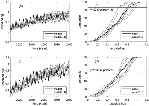
Figure 1(c) and (d) shows the same process to calculate the EV for specific humidity in the year 2080, which happens to correspond to the 73rd percentile for Model 1.

To extend the EV to include the dependence of climate variable uncertainties, this study defines the relationship between uncertainties in the climate variables as follows. In the case of the simple example of Figure 1, this requires the covariance of the uncertainties associated with the two variables shown in Figure 1(b) and (d) to be established. We define EVd as the covariance between two series of climate variables, where each series contains eight values of the same rank, as follows:

(4) $\begin{array}{rl}& \mathrm{E}\mathrm{V}{\mathrm{d}}_{\mathrm{z}\mathrm{g},\mathrm{h}\mathrm{u}\mathrm{s},\mathrm{m}{\mathrm{l}}_1,\mathrm{y}{\mathrm{r}}_{2080}}=cov\left\{\left(\mathrm{z}{\mathrm{g}}_{\mathrm{m}{\mathrm{l}}_1,p\mathrm{\_}86\mathrm{\%}},...,\mathrm{z}{\mathrm{g}}_{\mathrm{m}{\mathrm{l}}_8,p\mathrm{\_}86\mathrm{\%}}\right),\right.\\ & \left.\left(\mathrm{h}\mathrm{u}{\mathrm{s}}_{\mathrm{m}{\mathrm{l}}_1,p\mathrm{\_}73\mathrm{\%}},...,\mathrm{h}\mathrm{u}{\mathrm{s}}_{\mathrm{m}{\mathrm{l}}_8,p\mathrm{\_}73\mathrm{\%}}\right)\right\}\end{array}$(4)

The EVd is calculated separately for each point in time. The choice of which percentile to use for each variable is defined for each GCM of interest. It is also important to note that compared to the SREV, which was defined using the standard deviation of the model simulations, the EVd is defined as a covariance and, hence, the main diagonal of EVd is directly comparable to the square of the SREV (i.e. EV in the notation previously presented).

As will be explained in Section 3, in this study there are 72 simulations of four climate variables. Thus, EVd is calculated for each monthly time step using all 72 simulations. As there are four climate variables, a 4 × 4 covariance matrix defines the dependencies of the climate variables’ uncertainties for each monthly time step.

2.3 Incorporating climate variable uncertainty and dependence into statistical downscaling

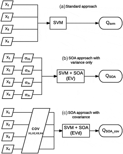
Eghdamirad et al. (2017) demonstrated the SOA framework using a support vector machine (SVM) as a regression model (Vapnik 1998) to estimate future streamflow using GCM projections. This simplified statistical downscaling process was chosen to illustrate the biases that can result if input uncertainty is ignored in a nonlinear climate system. The simplified SOA framework is now extended as an example to include the dependence of uncertainty. Details of the SVM model set-up specifically for this case study are provided in Section 3.

The process of applying SOA into the SVM model is presented in Equations (5), (6), and (7). All equations are for a single time step and the same process is performed for every monthly time step in the study period (2006–2100). In these equations, x_i is a predictor variable, $\mathrm{E}{\mathrm{V}}_{X_i}$is the uncertainty of variable x_i which is calculated from the vector of simulations X_i with the same ranking as x_i, EVd is the covariance matrix of the predictor set, and Q is the future projection of streamflow. Equation (5) shows the SVM estimated future projection of streamflow as follows:

(5) $E\left(Q\right)\approx \mathrm{S}\mathrm{V}\mathrm{M}\left(x_1,...,x_n\right)$(5)

Second-order approximation is used to modify Equation (5) by adding the second-order uncertainty term for each climate variable (Eghdamirad et al. 2017):

(6) $E\left(Q\right)\approx \mathrm{S}\mathrm{V}\mathrm{M}\left(x_1,...,x_n\right)+\frac{1}{2}\times \sum _{i=1}^n\frac{{\mathrm{\partial }}^2\mathrm{S}\mathrm{V}\mathrm{M}}{\mathrm{\partial }{x_i}^2}\times {\mathrm{E}\mathrm{V}}_{X_i}^{\hspace{0.17em}}$(6)

In this study, Equation (6) is expanded to include the dependence of the climate variable uncertainty which is measured by EVd as derived in the Section 2.2. The complete SOA implementation in the SVM model is as follows:

(7) $E\left(Q\right)\approx \mathrm{S}\mathrm{V}\mathrm{M}\left(x_1,...,x_n\right)+\frac{1}{2}\sum _{i=1}^n\sum _{j=1}^n\frac{{\mathrm{\partial }}^2\mathrm{S}\mathrm{V}\mathrm{M}}{\mathrm{\partial }{x}_i\mathrm{\partial }{x}_j}|\mathrm{E}\mathrm{V}\mathrm{d}\left[X_i,X_j\right]$(7)

Figure 2 shows the schematic of the standard SVM approach (Equation (5) in Fig. 2(a)), the SVM approach with SOA (Equation (6) in Fig. 2(b)), and finally the SVM approach with SOA considering the dependence of uncertainties across climate variables (Equation (7) in Fig. 2(c)).

Figure 2. Comparison of statistical downscaling of streamflow (Q) using: (a) the standard SVM approach; (b) the SVM approach with SOA and only uncertainties of climate variables; and (c) the SVM approach with SOA and dependence of uncertainties of climate variables.

To implement the expanded SOA analysis, a second derivative (or Hessian) of the SVM model is required. Because the analytical derivative of the SVM is complex (Lázaro et al. 2005), a numerical approximation of the derivative was implemented in this study. A numerical approximation of the Hessian matrix is calculated as the second derivative of the SVM, using the R computing platform. The numerical approximation of the Hessian is calculated as the Jacobian of the gradient using the R function “hessian” in the package “numDeriv”.

3 Case study

3.1 SVM model set-up

To demonstrate the new proposed framework in a sample case study, the SVM model used by Eghdamirad et al. (2017) is adopted in this study. The SVM regression model is calibrated with monthly streamflow and re-analysis data for two locations in Australia. An SVM has been proven to be effective in downscaling streamflow (Ghosh and Mujumdar 2008, Joshi et al. 2013, Sachindra et al. 2013). Following Eghdamirad et al. (2017), the SVM is used via the package “e1071” in the R computing platform using a radial basis function (RBF) as the kernel function. To avoid overfitting in the SVM, a 10-fold cross-validation is adopted by tuning the SVM with a grid-search method (Gold and Sollich 2003) with a range of values for epsilon of 0.01 to 1 and for cost 2 to 512. The root mean square error (RMSE) is used to select the best performance of the SVM.

The streamflow for two Australian Bureau of Meteorology (BOM) feature hydrological reference stations (Ajami et al. 2017) is used in this study and was chosen based on the different-sized catchments and different climate zones. The BOM has introduced seven feature reference stations to cover contrasting hydro-climate regions in Australia. The two stations were chosen in this study because of the good performance of the SVM model in predicting streamflow using current climate predictors at these two locations. The unregulated streamflow data (with minimal effects of water-resource development and land-use change) used here are available from http://www.bom.gov.au/water/hrs/feature.shtml. Details of the chosen hydrological reference stations and the time period of the SVM calibration are presented in Table 1.

Table 1. Characteristics of the hydrological stations.

Station	ID	State	Area (km^2)	Rainfall (mm)	Study period
					Start	End
Sardine Creek O’Brien Crossing	231213	Victoria	152	950	Jan-72	Dec-05
Yarragil Formation	614044	Western Australia	80	960	Jan-72	Dec-05

The downscaling predictor variables are selected from the GCM grid points that cover the catchments of interest. Based on the findings of Eghdamirad et al. (2017), four climate variables are selected in this study as predictors: geopotential height (zg), specific humidity (hus), eastward wind (ua), and northward wind (va). Unlike Eghdamirad et al. (2017), a single pressure level (500 hPa) is adopted to simplify the investigation. Selecting climate variables as predictors for any downscaling method is a function of the physical process they convey, as well as the statistical relationship they exhibit with the predictand (Fowler et al. 2007). So, correlation of climate variables may lead to selecting some and removing other similar climate variables (Najafi et al. 2011). The innovation of this work is that it quantifies the bias of downscaling due to the dependence of the uncertainty of the climate variables rather than correlating the variables, as traditionally assessed.

Re-analysis data for calibrating the SVM regression models were provided by the National Center for Environmental Prediction – National Center for Atmospheric Research (NCEP/NCAR). The calibrated SVM is used with GCM projections for the 21st century (2006–2100) to estimate future streamflow. Consistent with other studies about uncertainty of future GCMs (Hawkins and Sutton 2011, Fischer and Knutti 2015, Hegerl et al. 2015), a period of 95 years (2006–2100) is chosen for this study. These results are expected to change regionally and globally if the simulations are extended to 2300, due to the non-monotonic change in precipitation over time (Hawkins et al. 2014).

The future streamflow projections are based on the first ensemble of scenario RCP2.6 for model CSIROI-MK3-6-0. The GCM data are bias corrected using the re-analysis data and nested bias correction (NBC) (Johnson and Sharma 2012, Mehrotra and Sharma 2015, Mehrotra et al. 2018). The SVM model is calibrated using standardized streamflow and re-analysis data (standardized by subtracting the mean and dividing by the standard deviation). Because standardized responses are used in the SVM model, the final value of the future streamflow is calculated by rescaling with the mean and standard deviation of the observed streamflow.

For the purposes of calculating EVd, all the GCMs in CMIP5 that provided results for the three RCPs (RCP2.6, RCP4.5, RCP8.5) and three ensembles (r1i1p1, r2i1p1, r3i1p1) are used. These GCMs are CCSM4, CESM1 (CAM5), CSIRO-MK3-6-0, CanESM2, HadGEM2-ES, IPSL-CM5A-LR, MIROC5, and MPI-ESM-LR. To calculate EVd, a common grid is required for all GCMs. The re-analysis grid resolution was used (2.5° × 2.5° resolution) and GCMs were regridded using bilinear interpolation (Nawaz and Adeloye 2006). For the purposes of calculating the EVd and allowing the variables to be compared, the GCM projections are standardized by the current period mean and variance, thereby ensuring consistency in moments of orders one and two between the current period model simulations and observations.

3.2 Results

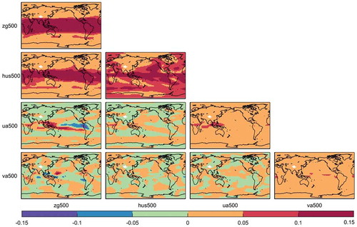
Figure 3 presents the EVd results using the described approach. The main diagonal shows the variance of each variable and is the EV. The other panels are the EVd as defined in Equation (4). As shown in Figure 3, there are strong patterns globally in the uncertainty dependence, with larger covariances at some locations. One would expect that the use of the proposed complete SOA implementation in the SVM model with covariance (SOA_cov) would be more effective in these locations. In particular, the uncertainty of geopotential height and specific humidity show strong interactions in the tropics. Figure 3 presents the EVd averaged over all of the months during the analysis period. The seasonal cycle of moisture availability is also obvious in these interactions. Average uncertainty and dependence for January and July are provided in the supplementary information (Figs S1 and S2), confirming that the temporally varying dependence seen for the study locations also occurs globally. It is clear that the EVd is small for all variables over Australia, unlike the case of northern Africa or South America. However, as previously mentioned, based on Eghdamirad et al. (2017), the same set of predictors and streamflow were adopted as an example to demonstrate the new proposed framework of this study. The main difference from this previous study is that in the former the predictors were selected from two pressure levels of 500 and 850 hPa, but in the current study all the predictors are selected at a 500-hPa pressure level to simplify the demonstration of the covariance matrix.

Figure 3. Global spatial distribution of monthly averaged uncertainty and its cross-variable dependence (EVd) for standardized climate variables of geopotential height (zg), specific humidity (hus), eastward wind (ua), and northward wind (va). The maps are for the first ensemble of scenario RCP2.6 using model CSIROI-MK3-6-0. The main diagonal shows the error variance for each variable and the lower triangle the EVd values.

The EVd is used as the basis for downscaling monthly streamflow for two study locations from the states of Victoria and Western Australia as detailed in Table 1 with the results presented in Table 2 and Figure 4. Table 2 presents the mean observed and simulated monthly streamflow (Fig. S3 of the Supplementary information compares the time series of the SVM simulation of streamflow to the observed streamflow at both locations). The mean streamflow is reasonably well represented by the SVM model. The highest monthly totals are underestimated by the SVM although the timing of the peak flows and low flows is captured well. As the focus of this study is to investigate the importance of considering dependence in uncertainty estimates for downscaling, we found that the SVM provides a simple modelling alternative that operated satisfactorily for the monthly streamflow downscaling problem under study.

Table 2. SVM, SOA, and SOA_cov approximation of mean monthly streamflow (ML) for two feature hydrological stations. For the Current, Diff (%) relates to the difference between observed and SVM values. For the Future, Diff (%) relates to the difference between the SVM with SOA and SVM with SOA_cov.

Station	Monthly discharge (ML)
	Current			Future
	Observed	SVM	Diff (%)	SVM	SOA	Diff (%)	SOA_cov	Diff (%)
231213	2312	2293	−0.8	2269	2306	1.6	2284	0.7
614044	159	147	−7.3	151	154	1.7	154	1.6

It should be noted that streamflow and GCM ensembles are not contemporaneous. It is therefore not possible to evaluate the SVM and SOA models using historical GCM simulations. The issue of evaluating SOA by comparing historical data and future data is also impacted by the multiple sources of uncertainty present, which are not all present in historical simulations. This research aims to quantify the potential bias that may occur by ignoring the uncertainty of climate variables and the implications of this dependence in uncertainty in statistical downscaling. This bias depends on the uncertainty and its characterization across variables. For historical data, there is no scenario uncertainty or ensemble uncertainty when the SVM is calibrated with re-analysis data. Thus, the sources of bias in future simulations are not the same as the historical simulations.

The future streamflow projections using the SVM, SOA, and SOA with covariance (SOA_cov) are compared as shown in Table 2. Both SOA and SOA_cov modify the mean streamflow compared to that when uncertainty is ignored (SVM base case). As can be seen in Table 2, the increases in streamflow introduced by SOA are slightly modulated by the SOA_cov method. To evaluate the impact of the SOA_cov method across the full distribution of the modelled streamflow, quantile–quantile plots (QQ plots) of future projections of monthly streamflow using the SVM, SOA, and SOA_cov were developed and are shown in Figure 4. Eghdamirad et al. (2017) showed that ignoring the uncertainty of predictors causes a noticeable bias in the low-flow estimates. Figure 4 illustrates that, when the uncertainty dependence is incorporated using the SOA_cov approach, the low flows continue to be the most affected by the uncertainty and its dependence. Table 3 shows the influence of the uncertainty and dependence of the uncertainty on low flows. For the two case-study locations, incorporating uncertainty in the predictors leads to slightly higher streamflow estimates, with greater increases in the low flow or drought period simulations. This has implications for future drought management, and highlights the need for considering the SOA or SOA_cov approach in assessing climate change impacts.

Table 3. Streamflow projections of low quantiles using the SVM, SOA, and SOA_cov simulations for streamflow stations 231213 and 614044.

	Quantile
	1%	2%	3%	4%	5%	7.5%	10%	15%	20%
Station 231213
SVM	0	0	158	248	334	474	581	769	899
SOA	0	0	236	316	389	538	646	821	959
SOA_cov	0	1	233	315	376	515	629	804	937
Station 614044
SVM	62	380	559	670	722	826	918	1069	1206
SOA	144	522	655	745	799	904	977	1137	1266
SOA_cov	110	528	660	737	793	897	979	1124	1259

Figure 4. QQ plots comparing streamflow projections using the SVM, SOA, and SOA_cov simulations for streamflow stations 231213 and 614044 (details in Table 1).

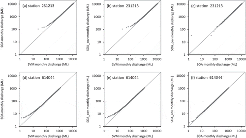
The additional changes from incorporating uncertainty dependence (Fig. 4, right column) are small compared to the biases that result from completely neglecting uncertainty (Fig. 4, middle column). There are a few interesting differences between the SOA and SOA_cov projections at the two locations considered. Table 2 shows that for average flow there are not any significant differences between SOA and SOA_cov. However, as seen in Fig. 4(c) and (f), for low flows, it was found that incorporating dependence of uncertainties causes lower streamflow in the SOA_cov simulation compared to that of the SOA simulation at station 231213. However, for station 614044, the SOA_cov simulations for low flows are higher than those of SOA.

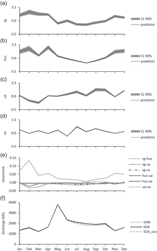
To examine the differences among the SVM, SOA, and SOA_cov simulations in more detail, Figure 5 shows the time series of the projections of SVM, SOA, and SOA_cov for 2090, as an example, at station 231213. For all input variables, the uncertainty varies throughout the year (Fig. 5(a)–(d)). The largest differences between the SVM, SOA, and SOA_cov projections occur simultaneously with the high uncertainty in the eastward wind (ua). The SOA_cov projections are slightly lower than those of the SOA simulations. Figure 5(e) shows the uncertainty covariance for all of the pairs of variables. The covariance terms including geopotential height during the early part of the year offset each other with both negative and positive interactions. However, between July and October, including dependence in the variable uncertainty leads to some differences in the projections, which seem to be due to the eastward wind component. Further work is required to separate the contribution of the model sensitivity to each of the predictors (model partial derivative in Equation (7)) to these differences from the contribution of the uncertainties and their dependences.

Figure 5. Comparison of uncertainties of predictors and dependence of uncertainty over time using simulations of streamflow at station 231213 for the year 2090. (a)–(d) predictors of geopotential height (zg), specific humidity (hus), eastward wind (ua) and northward wind (va), respectively, with their 90th percentile confidence limits; (e) dependence of uncertainties; and (f) the simulations of SVM, SOA, and SOA_cov.

4 Summary and conclusions

This research proposes a new framework to apply uncertainties of climate variables and the dependence of their uncertainties into monthly statistical downscaling of streamflow. For simplicity of demonstration, only four climate variables (geopotential height, specific humidity, eastward wind, and northward wind) were used as predictors at only one pressure level of 500 hPa to downscale monthly streamflow for two hydrological stations in Australia. This study provides a framework to investigate and quantify the importance of the bias that results from ignoring the uncertainties of predictors and their dependence. It is expected the obtained results would change if a broader range of climate variables was used and the study was applied to regions of different hydroclimatology. A new metric termed EVd has been introduced to estimate the dependence of the climate variables’ uncertainties. These new estimates of climate variable uncertainties can be incorporated into the SVM projection of streamflow for the 21st century using an expanded SOA approach that accounts for the covariance of input variable uncertainty. Although the extended SOA only leads to small differences in the streamflow projections compared to a case assuming independent uncertainty, these small differences are due to the relatively low dependence found over the study region. In other parts of the world there are strong interactions in the uncertainties of different climate variables, in particular in the tropics. Ignoring these interactions might lead to additional biases in downscaling simulations, because of the nonlinearity of the relationship between predictors and streamflow. It is therefore recommended that the SOA with covariance be adopted to ensure that climate change impact assessments are not biased by ignoring climate variable uncertainty and its dependence.

Acknowledgements

We acknowledge the World Climate Research Programme’s Working Group on Coupled Modelling, which is responsible for the CMIP, and we would like to thank the climate modelling groups for producing and making available their model output. For the CMIP, the US Department of Energy’s Program for Climate Model Diagnosis and Intercomparison provided coordinating support and led development of software infrastructure in partnership with the Global Organization for Earth System Science Portals. NCEP re-analysis data were provided by the National Oceanic and Atmospheric Administration, Office of Oceanic and Atmospheric Research, Earth System Research Laboratory, Physical Sciences Division Boulder, Colorado, USA (http://www.esrl.noaa.gov/psd/data/gridded). Hydrological data were provided by the Australian Bureau of Meteorology (http://www.bom.gov.au/water/hrs/feature.shtml).

Disclosure statement

No potential conflict of interest was reported by the authors.

Supplementary material

Supplementary data for this article can be accessed here.

Additional information

Funding

This work was supported by a grant from National Research Foundation (NRF) of Korea, funded by the Korean government (MSIP) (No. 2016R1A2A1A05005306).

References

- Ajami, H., et al., 2017. On the non-stationarity of hydrological response in anthropogenically unaffected catchments: an Australian perspective. Hydrology and Earth System Sciences, 21, 281–294. doi:10.5194/hess-21-281-2017
- Alvisi, S. and Franchini, M., 2010. Pipe roughness calibration in water distribution systems using grey numbers. Journal of Hydroinformatics, 12, 424. doi:10.2166/hydro.2010.089
- Benjamin, J. and Cornell, C., 1970. Reliability, statistics and decision for civil engineers. New York: McGraw Hill.
- Bergant, K. and Kajfež-Bogataj, L., 2005. N–PLS regression as empirical downscaling tool in climate change studies. Theoretical and Applied Climatology, 81, 11–23. doi:10.1007/s00704-004-0083-2
- Braunisch, V., et al., 2013. Selecting from correlated climate variables: a major source of uncertainty for predicting species distributions under climate change. Ecography, 36, 971–983. doi:10.1111/j.1600-0587.2013.00138.x
- Dettinger, M.D. and Wilson, J.L., 1981. First order analysis of uncertainty in numerical models of groundwater flow part: 1. Mathematical development. Water Resources Research, 17, 149–161. doi:10.1029/WR017i001p00149
- Eghdamirad, S., Johnson, F., and Sharma, A., 2017. Using second-order approximation to incorporate GCM uncertainty in climate change impact assessments. Climatic Change, 142, 37–52. doi:10.1007/s10584-017-1944-x
- Eghdamirad, S., et al., 2016. Quantifying the sources of uncertainty in upper air climate variables. Journal of Geophysical Research: Atmospheres, 121, 3859–3874.
- Fischer, E.M. and Knutti, R., 2015. Anthropogenic contribution to global occurrence of heavy-precipitation and high-temperature extremes. Nature Climate Change, 5, 560–564. doi:10.1038/nclimate2617
- Fowler, H.J., Blenkinsop, S., and Tebaldi, C., 2007. Linking climate change modelling to impacts studies: recent advances in downscaling techniques for hydrological modelling. International Journal of Climatology, 27, 1547–1578. doi:10.1002/(ISSN)1097-0088
- Fowler, K.J.A., et al., 2016. Simulating runoff under changing climatic conditions: revisiting an apparent deficiency of conceptual rainfall-runoff models. Water Resources Research, 52, 1820–1846. doi:10.1002/2015WR018068
- Ghosh, S. and Mujumdar, P.P., 2008. Statistical downscaling of GCM simulations to streamflow using relevance vector machine. Advances in Water Resources, 31, 132–146. doi:10.1016/j.advwatres.2007.07.005
- Gold, C. and Sollich, P., 2003. Model selection for support vector machine classification. Neurocomputing, 55, 221–249. doi:10.1016/S0925-2312(03)00375-8
- Haan, C.T., 2002. Statistical methods in hydrology (2nd ed.). Iowa State: Blackwell Publishing.
- Hawkins, E., Joshi, M., and Frame, D., 2014. Wetter then drier in some tropical areas. Nature Climate Change, 4, 646–647. doi:10.1038/nclimate2299
- Hawkins, E., et al., 2015. Irreducible uncertainty in near-term climate projections. Climate Dynamics, 46, 3807–3819. doi:10.1007/s00382-015-2806-8
- Hawkins, E. and Sutton, R., 2009. The potential to narrow uncertainty in regional climate predictions. Bulletin of the American Meteorological Society, 90, 1095–1107. doi:10.1175/2009BAMS2607.1
- Hawkins, E. and Sutton, R., 2010. The potential to narrow uncertainty in projections of regional precipitation change. Climate Dynamics, 37, 407–418. doi:10.1007/s00382-010-0810-6
- Hawkins, E. and Sutton, R., 2011. The potential to narrow uncertainty in projections of regional precipitation change. Climate Dynamics, 37, 407–418. doi:10.1007/s00382-010-0810-6
- Hegerl, G.C., et al., 2015. Challenges in quantifying changes in the global water cycle. Bulletin of the American Meteorological Society, 96, 1097–1115. doi:10.1175/BAMS-D-13-00212.1
- Johnson, F. and Sharma, A., 2012. A nesting model for bias correction of variability at multiple time scales in general circulation model precipitation simulations. Water Resources Research, 48.
- Joshi, D., et al., 2013. Databased comparison of sparse bayesian learning and multiple linear regression for statistical downscaling of low flow indices. Journal of Hydrology, 488, 136–149. doi:10.1016/j.jhydrol.2013.02.040
- Lázaro, M., et al., 2005. Support vector regression for the simultaneous learning of a multivariate function and its derivatives. Neurocomputing, 69, 42–61. doi:10.1016/j.neucom.2005.02.013
- Mehrotra, R., Johnson, F., and Sharma, A., 2018. A software toolkit for correcting systematic biases in climate model simulations. Environmental Modelling & Software, 104, 130–152. doi:10.1016/j.envsoft.2018.02.010
- Mehrotra, R. and Sharma, A., 2015. Correcting for systematic biases in multiple raw GCM variables across a range of timescales. Journal of Hydrology, 520, 214–223. doi:10.1016/j.jhydrol.2014.11.037
- Najafi, M., Moradkhani, H., and Jung, I., 2011. Assessing the uncertainties of hydrologic model selection in climate change impact studies. Hydrological Processes, 25, 2814–2826. doi:10.1002/hyp.v25.18
- Nawaz, N.R. and Adeloye, A.J., 2006. Monte Carlo assessment of sampling uncertainty of climate change impacts on water resources yield in Yorkshire, England. Climatic Change, 78, 257–292. doi:10.1007/s10584-005-9043-9
- Panda, D.K., et al., 2008. Improved estimation of soil organic carbon storage uncertainty using first-order Taylor series approximation. Soil Science Society of America Journal, 72, 1708. doi:10.2136/sssaj2007.0242N
- Sachindra, D.A., et al., 2013. Least square support vector and multi-linear regression for statistically downscaling general circulation model outputs to catchment streamflows. International Journal of Climatology, 33, 1087–1106. doi:10.1002/joc.v33.5
- Tebaldi, C. and Knutti, R., 2007. The use of the multi-model ensemble in probabilistic climate projections. Philosophical Transactions of the Royal Society A: Mathematical, Physical and Engineering Sciences, 365, 2053–2075. doi:10.1098/rsta.2007.2076
- Van Vuuren, D.P., et al., 2011. The representative concentration pathways: an overview. Climatic Change, 109, 5–31. doi:10.1007/s10584-011-0148-z
- Vapnik, V.N., 1998. Statistical learning theory Wiley. New York, 156–160.
- Wang, S.-J. and Hsu, K.-C., 2009. The application of the first-order second-moment method to analyze poroelastic problems in heterogeneous porous media. Journal of Hydrology, 369, 209–221. doi:10.1016/j.jhydrol.2009.02.049
- Woldemeskel, F.M., et al., 2012. An error estimation method for precipitation and temperature projections for future climates. Journal of Geophysical Research: Atmospheres, 117.
- Woldemeskel, F.M., et al., 2016. Quantification of precipitation and temperature uncertainties simulated by CMIP3 and CMIP5 models. Journal of Geophysical Research: Atmospheres, 121, 3–17.
- Xue, D., et al., 2010. Error assessment of nitrogen and oxygen isotope ratios of nitrate as determined via the bacterial denitrification method. Rapid Commun Mass Spectrom, 24, 1979–1984. doi:10.1002/rcm.4604
- Xue, J., Leung, Y., and Ma, J.-H., 2015. High-order Taylor series expansion methods for error propagation in geographic information systems. Journal of Geographical Systems, 17, 187–206. doi:10.1007/s10109-014-0207-x
- Yip, S., et al., 2011. A simple, coherent framework for partitioning uncertainty in climate predictions. Journal of Climate, 24, 4634–4643. doi:10.1175/2011JCLI4085.1