Numerical modelling-based comparison of longitudinal dispersion coefficient formulas for solute transport in rivers

ABSTRACT

River water quality models usually apply the Fischer equation to determine the longitudinal dispersion coefficient (D_x) in solving the advection–dispersion equation (ADE). Recently, more accurate formulas have been introduced to determine D_x in rivers, which could strongly affect the accuracy of the ADE results. A numerical modelling-based approach is presented to evaluate the performance of various D_x formulas using the ADE. This approach consists of a finite difference approximation of the ADE, a MATLAB code and a MS Excel interface; it was tested against the analytical ADE solution and demonstrated using eight well-known D_x formulas and tracer study data for the Chattahoochee River (USA), the Severn (UK) and the Athabasca (Canada). The results show that D_x has an important effect on tracer concentrations simulated with the ADE. Comparison between the simulated and measured concentrations confirms the appropriate performance of Zeng and Huai’s formula for D_x estimation. Use of the newly proposed equations for D_x estimation could enhance the accuracy of solving the ADE.

KEYWORDS:

• advection–dispersion equation
• longitudinal dispersion coefficient
• real-field cases
• water quality modelling

Editor S. Archfield Associate editor X. Fang

1 Introduction

Rivers play a significant role in water supply for municipal, agricultural and industrial purposes. In the meantime, rivers also receive pollutants from diverse sources in drainage basins. These pollutants have led to the degradation of river water quality (RWQ). Thus, having reliable information about RWQ is a prerequisite for appropriately managing rivers (Noori et al. 2019). While pollutants are dispersed longitudinally, laterally and vertically through diffusive and advective transport processes, longitudinal dispersion is the governing process for the concentration gradient along rivers where the cross-sectional mixing is completed (Fischer et al. 1979, Seo and Cheong 1998). In this regard, one-dimensional (1D) mathematical models, which allow the fate of pollutants to be simulated, are widely used to address RWQ degradation (Rauch et al. 1998). Mass and pollutant transport in natural open channels is generally governed by the advection–dispersion equation (ADE). There are analytical and numerical approaches to predict pollutant transport by solving the ADE. To that end, hydraulic conditions should be correctly simulated. In addition, the Fickian-type assumptions under the ADE (e.g. there is a balance between diffusion and advection) should be valid (Fischer et al. 1979, Seo and Cheong 1998). However, analytical solutions are valid under prismatic and simple channel geometries and flow and solute conditions. Solute transport in a natural river is governed by a suite of complex hydraulic and geochemical processes, such as mixing, exchange with storage zones and biogeochemical reactions (Deng et al. 2002). These factors make the dispersion process different in idealized cases compared to real rivers. Therefore, the application of analytical solutions is just limited to the idealized cases with simple geometrics. Unlike the analytical approaches, numerical solutions have been widely applied to simulate RWQ in real-world engineering problems. In this regard, many 1D executive codes and commercial water quality programs, such as QUAL2K (Chapra et al. 2003), WASP (Di Toro et al. 1983), MIKE11 (Havnø et al. 1995), MASCARET (Goutal et al. 2012) and HEC-RAS (USACE 1986), have been introduced.

A major parameter involved in the 1D models is the longitudinal dispersion coefficient (D_x). The parameter D_x, involved in all RWQ models, is generally treated as an unknown parameter to be determined (El Kadi Abderrezzak et al. 2015, Parsaie and Haghiabi 2017a). In other words, when the ADE model is applied to predict pollutants in natural streams, the selection of a proper D_x value is required. Measurements have shown that D_x commonly has large variations (Seo and Cheong 1998). Since D_x cannot be measured directly, and tracer injection tests for indirect estimation of D_x are often time consuming and costly, empirical equations have been widely employed to calculate D_x for natural open channels (Park and Lee 2001, El Kadi Abderrezzak et al. 2015). These equations have mainly been formulated based on some available hydraulic-geometric parameters, such as the cross-sectional averaged velocity (U), shear velocity (U*), flow depth (d) and channel width (W) (Balf et al. 2018).

In spite of the availability of a large number of empirical equations for D_x estimation, some of the most well-known RWQ models apply, by default, the original formula proposed by Fischer (1975) to determine D_x in the ADE solution process. Since the publication of Fisher’s equation in 1975, new and more accurate formulas have been introduced for determining D_x (Park and Lee 2001, Deng et al. 2002, Kashefipour and Falconer 2002, Sahay and Dutta 2009, Etemadshahidi and Taghipour 2012, Zeng and Huai 2014, Sattar and Gharabaghi 2015, Haghiabi 2016, Alizadeh et al. 2017a). Therefore, there is a need to assess the formulas and identify the most effective ones with a computational program. In this regard, the overall goal of this study is to evaluate the effect of application of different formulas for D_x estimation on the ADE performance. To achieve this goal, a variety of well-known formulas for D_x estimation (Fischer 1975, Iwasa and Aya 1991, Seo and Cheong 1998, Deng et al. 2001, Kashefipour and Falconer 2002, Sahay and Dutta 2009, Etemadshahidi and Taghipour 2012, Zeng and Huai 2014) were considered. All of these formulas are based on some effective hydraulic-geometric parameters on D_x. Seo and Cheong (1998), by conducting a dimensional analysis, showed that D_x is highly influenced by five parameters, including the Reynolds number, W∕d, U∕U* and lateral and vertical irregularities. By considering turbulent flow in natural rivers, the Reynolds number can be ignored (Chow 1973). In addition, the parameter U∕U* can properly represent the effect of lateral and vertical irregularities (Seo and Cheong 1998). Thus, almost all researchers have tried to present an empirical formula for D_x estimation based on the same variables: W, d, U and U*.

However, different researchers applied different regression techniques to tune their formulas for D_x estimation. In addition, they did not use the same datasets, resulting in different D_x formulas with varying performance. While several formulas for D_x estimation have been proposed, few published papers have aimed to evaluate how the application of different formulas affects the results from an ADE-based model. El Kadi Abderrezzak et al. (2015) developed a computational control volume approach for simulating the non-reactive solute transport process in 1D streams in both steady and unsteady conditions. Also, an extension of the Telemac-Mascaret (an integrated open source computational software), developed by Goutal et al. (2012), was used to apply some D_x formulas. While their study provided interesting results in the field of RWQ modelling, there are still some barriers to remove. For example, dozens of D_x formulas have been published in recent years (Alizadeh et al. 2017b). Here we aim to use some of the new formulas that have not been evaluated in previous studies. It is important to develop a proper RWQ model to simulate pollutant transport in 1D water bodies by using the new formulas for estimating D_x.

In the following section, the ADE is discussed regarding analytical and numerical approaches, the structure of the developed code and the user-interface of the model are described, and three real-field cases are introduced. The findings are given in Section 3, followed by our conclusions in Section 4.

2 Materials and methods

2.1 Advection–dispersion equation (ADE)

The transport process of dissolved conservative materials in 1D water bodies is considered as a superposition of two fundamental physical processes: advection and dispersion. Mathematically, the advection and dispersion processes of a reactive solute after passing the initial mixing length can be described with the following advection and dispersion equation (Ghane et al. 2016, Noori et al. 2016, 2017, Parsaie and Haghiabi 2017b):

(1) $\frac{\mathrm{\partial }C}{\mathrm{\partial }t}=-U\frac{\mathrm{\partial }C}{\mathrm{\partial }x}+\frac{\mathrm{\partial }}{\mathrm{\partial }x}\left(D_x\frac{\mathrm{\partial }C}{\mathrm{\partial }x}\right)+P-kC$(1)

where C is the cross-sectional average concentration (mg L⁻¹), U is the cross-sectional average velocity (m s⁻¹), P is the source/sink term, and k is chemical degradation rate (d⁻¹). In Equation (1), $U(\mathrm{\partial }C/\mathrm{\partial }x)$ is the advection term that causes the body movement of a constituent dissolved in water. The term $\frac{\mathrm{\partial }}{\mathrm{\partial }x}\left(D_x\frac{\mathrm{\partial }C}{\mathrm{\partial }x}\right)$ represents dispersive transport, which is the cause of the solute being spread as it passes through the water column.

In the absence of sink/source and diffusion terms, Equation (1) can be solved analytically for the pure advection process as a plug flow, as shown in Equation (2) (Chapra 1997). The basic assumptions for Equation (2) include uniform flow and fully mixing solute in the channel:

(2) $C=C_0\mathrm{e}\mathrm{x}\mathrm{p}(kt)$(2)

where t = x/U is the travel time downstream of the source injection point, x is the distance to the point source (m), and C₀ is the concentration at t = 0.

Equation (1) can be solved analytically in the form of Equation (3) under the assumptions that: (a) the sink/source term is neglected (Chapra 1997); (b) the flow is uniform; and (c) the solute is fully mixed with a constant D_x in the channel.

(3) $C=\frac{m_p}{2\sqrt{\pi D_{x}t}}\mathrm{e}\mathrm{x}\mathrm{p}\left[\frac{{\left(x-Ut\right)}^2}{4D_{x}t}-kt\right]$(3)

where m_p is the total mass of solute passing through a unit area of cross-section (g m⁻²). In this solution, the substance is initially fully mixed across the section and released at x = 0. Accordingly, the solution for a pure diffusion process (e.g. Fick’s second law), is described by series of bell-shaped curves that spread out over time symmetrically. Moreover, the effect of advection (for ADE) is to shift the dispersion solution bodily downstream at velocity U.

2.2 Numerical scheme

The numerical solution space is discretized in Figure 1, where the concentration c_i^l+1 is the target. The ADE (Equation (1)) is discretized using a first-order forward difference scheme for the time derivative, a first-order backward difference for the first spatial derivative (assumed), and a second-order symmetric difference for the second spatial derivative. After plugging them into Equation (1) and collecting terms, the process yields Equation (4) (Chapra 1997):

(4) $\begin{array}{rl}& C_i^{l+1}=\frac{P_i^l}{V_i}-\frac{\mathrm{\Delta }t}{V_i}\left(-Q_{i-1,i}{\alpha }_{i-1,i}-E_{i-1,i}\right)C_{i-1,i}^l\\ & +\left[1-\frac{\mathrm{\Delta }t}{V_i}\left(-Q_{i-1,i}{\beta }_{i-1,i}+Q_{i,i+1}{\alpha }_{i,i+1}+E_{i-1,i}+E_{i,i+1}+k_i{V}_i\right)\right]C_i^l\\ & -\frac{\mathrm{\Delta }t}{V_i}\left(Q_{i,i+1}{\beta }_{i,i+1}-E_{i,i+1}\right)C_{i+1}^l\end{array}$(4)

Figure 1. Computational space for the explicit method considered in this research.

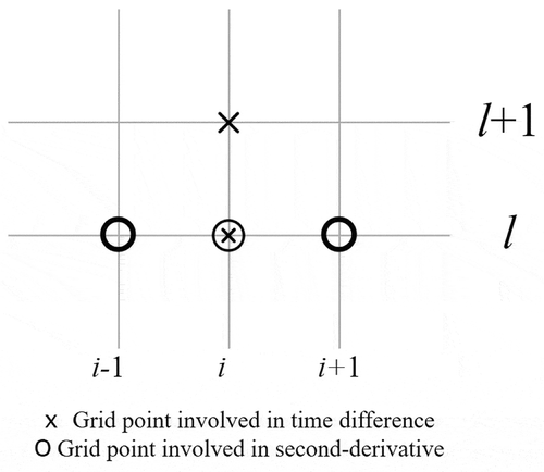
In Equation (4), l refers to the time step, i denotes the spatial step, V is the segment volume (m³), Q = U.A is river discharge (m³ s⁻¹), α and β are dimensionless weighting parameters ranging from 0 to 1 for manipulating the numerical errors, and $E=\left(D_x\times A\right)/\mathrm{\Delta }x$ where A is cross-sectional area of flow (m²).

This discretization is based on a forward time and backward space scheme for α = 1.0 and forward time and central space scheme for α = 0.5. Double subscript terms refer to interfaces between two adjacent volumes; e.g. the term Q_i-1,i refers to the flow between volumes i – 1 and i.

To satisfy the stability condition, the following criterion is used (Chapra 1997, Szymkiewicz 2010):

(5) $\mathrm{\Delta }t<\frac{{\left(\mathrm{\Delta }x\right)}^2}{U\mathrm{\Delta }x\left(\alpha -\beta \right)+2D_x+k{\left(\mathrm{\Delta }x\right)}^2}$(5)

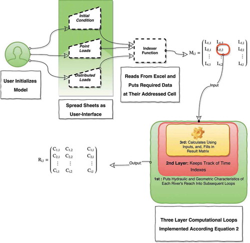
To implement Equation (4) in MS Excel, a MATLAB code was constructed. For this purpose, a matrix of solutions was considered for this equation. The matrix consists of rows (equal spatial steps) and columns (equal time steps). The number of columns is equal to the travel time divided by the selected time step and the number of rows is the result of dividing the length of river by the chosen spatial step. The first row of the resulting matrix practically includes initial conditions and the first and last columns represent the boundary conditions. Performed tests indicated that the developed MATLAB code was able to solve the ADE under complex initial conditions of steady timed point loadings (STPL), impulse point loadings (IPL), distributed loadings (DL) and point-distributed loadings, simultaneously. In this regard, first, the user should specify the beginning and the end times of loading, the amount of discharging mass within the channel and other information that is required for solving Equation (1), such as loading type, geometric–hydraulic characteristics of the river, assigning a formula for D_x, initial and boundary conditions, and minimum and maximum of ∆t and ∆x. In this study, a variety of well-known formulas for D_x estimation were considered (Table 1).

Table 1. Summary of the selected D_x formulas.

Author(s)	Formula
Fischer (1975)	$\frac{D_x}{d{U}^{\ast }}=0.11{\left(\frac{W}{d}\right)}^2{\left(\frac{U}{U^{\ast }}\right)}^2$
Iwasa and Aya (1991)	$\frac{D_x}{d{U}^{\ast }}=2{\left(\frac{W}{d}\right)}^{1.5}$
Seo and Cheong (1998)	$\frac{D_x}{d{U}^{\ast }}=5.195{\left(\frac{W}{d}\right)}^{0.62}{\left(\frac{U}{U^{\ast }}\right)}^{1.428}$
Deng et al. (2001)	$\frac{D_x}{d{U}^{\ast }}=\left(\frac{0.15}{8\epsilon }\right){\left(\frac{W}{d}\right)}^{1.67}{\left(\frac{U}{U^{\ast }}\right)}^2$$\frac{D_x}{d{U}^{\ast }}=\left(\frac{0.15}{8\epsilon }\right){\left(\frac{W}{d}\right)}^{1.67}{\left(\frac{U}{U^{\ast }}\right)}^2\frac{-b\pm \sqrt{b^2-4ac}}{2a}$
Kashefipour and Falconer (2002)	$\frac{W}{d}\ge 50\to \frac{D_x}{d{U}^{\ast }}=10.612{\left(\frac{U}{U^{\ast }}\right)}^2$$\frac{W}{d}\le 50\to \frac{D_x}{d{U}^{\ast }}=\left(7.428+1.775{\left(\frac{W}{d}\right)}^{0.62}{\left(\frac{U^{\ast }}{U}\right)}^{0.572}\right){\left(\frac{U}{U^{\ast }}\right)}^2$
Sahay and Dutta (2009)	$\frac{D_x}{d{U}^{\ast }}=2{\left(\frac{W}{d}\right)}^{0.96}{\left(\frac{U}{U^{\ast }}\right)}^{1.25}$
Etemadshahidi and Taghipour (2012)	$\frac{W}{d}<30.6\to \frac{D_x}{d{U}^{\ast }}=15.49{\left(\frac{W}{d}\right)}^{0.78}{\left(\frac{U}{U^{\ast }}\right)}^{0.11}$$\frac{W}{d}\ge 30.6\to \frac{D_x}{d{U}^{\ast }}=14.12{\left(\frac{W}{d}\right)}^{0.61}{\left(\frac{U}{U^{\ast }}\right)}^{0.85}$
Zeng and Huai (2014)	$\frac{D_x}{dU}=5.4{\left(\frac{W}{d}\right)}^{0.7}{\left(\frac{U}{U^{\ast }}\right)}^{0.13}$

In the next step, considering the travel time and spatial step, the code organizes the entered data as two matrices, the matrix of discharged mass and the matrix of initial conditions. Then, the developed MATLAB code goes through the iterative numerical solution process. For this purpose, a MATLAB function, called the INDEXER, was developed. Given the time and position of the calculating cell, this function reads the related number from the above matrices (STPL, IPL and DL) and transfers the result to the computation cycle. Figure 2 presents a schematic view of the calculation workflow of the code developed in the MATLAB environment.

Figure 2. Components and architecture of the proposed model.

2.3 User-interface of model

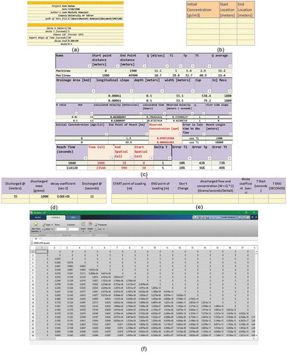
A user-friendly working interface was developed in MS Excel for modelling solute transport in uniform flow under STPL and DL loadings. The interface consists of five different worksheets.

1. Setting sheet (Fig. 3(a)): Completing some parts of this sheet is optional and just a few required cells should be filled: one may define the project name, implementation date, user name, the directory for saving the results and the company name. However, one must define ∆t, ∆x, α and the decay coefficient, and choose a formula for D_x (here shown by LDC), as well.

2. Initial condition sheet (Fig. 3(b)): Under initial conditions, the user should specify the initial concentration and injection end points.

3. Reach properties sheet (Fig. 3(c)): To properly simulate the solute concentration variation along a river, the user must complete all parts of this sheet on the hydraulic–geometric characteristics of the river and its tributaries. The sections highlighted in red are the ones that will be calculated by the model.

4. IPL loading sheet (Fig. 3(d)): The discharge mass, decay coefficient, and the time and location of discharge from the starting point are defined here. The model can simulate more than one solute constituent simultaneously. In this case, the decay coefficients for other solutes, if any, need to be defined. If not, the model will allocate the introduced decay coefficient in the setting sheet.

5. STPL and DL loadings sheet (Fig. 3(e)): This sheet provides the simulation of solute transport under the conditions of STPL and DL loadings and should be completed by the user. As the model could simulate more than one solute simultaneously, the decay coefficients for other solutes, if any, should be defined. If not, the model uses the introduced decay coefficient in the setting sheet.

6. Results sheet (Fig. 3(f). Finally, the results sheet presents the outcome.

Figure 3. Schematic view of the different parts of the working space of the model in the MS Excel environment.

2.4 Case studies

Three case studies were chosen to check the performance of the developed model: (a) the Athabasca River, Canada, for checking the model robustness on the solute transport resulting from the STLP condition; (b) the Chattahoochee River, and (c) the River Severn, located, respectively, in the USA and the UK, to evaluate the model performance on solute transport resulting from the IPL condition. These three rivers have different hydraulic, hydrological and geometric conditions. Solute transport in these rivers is governed by a suite of complex processes, such as mixing, exchange with storage zones, shearing advection, lateral mixing, hyporheic exchange, and effective diffusion in bottom sediment. Also, the average relative error (ARE) and the Nash-Sutcliffe efficiency criterion (NSE; Nash and Sutcliffe 1970) were used to check the performance of the developed models. Values of ARE and NSE equal to 0 and 1, respectively, correspond to a perfect match of the simulated concentrations to the measured ones, while values of −∞ and +∞ determine the worst model performance.

2.4.1 Athabasca River

The Athabasca River, the longest river in Alberta, originates from the Columbia Mountains, Canada (Shakibaeinia et al. 2016). Putz and Smith (2000) conducted a tracer study on the Athabasca River under STPL conditions. A fixed concentration of 2.3 × 10⁵ mg L⁻¹ of the tracer Rhodamine, with a constant rate of 1.3 × 10^–4 mg L⁻¹ s⁻¹, was gradually introduced into the river during a period of 5 h. Table 2 shows the peak solute concentrations measured at several stations along a 26-km reach of the river downstream of the injection point. According to Table 2, there is a decreasing trend in concentration in the equilibrium zone (near-field and mid-field of injection point) due to vertical and transverse mixing in the river. About 11 km downstream of the injection point (stations 14–18), the concentration becomes constant. This means that the solute becomes well mixed in the vertical and transverse directions.

Table 2. Flow and tracer test data collected on the Athabasca River (flow rate: 363.6 m³ s⁻¹). Dist.: distance from injection point.

Station	Dist. (km)	Flow (m^3/s)	Time (h)	Slope (1/100)	Depth (m)	Width (m)	Observed concentration (ppm)
St1	0.1	364	0.0217	1.3	2.88	102	0.00205
St2	0.3	364	0.0651	1.29	2.6	100	0.00164
St3	0.5	364	0.1085	1.5	1.58	162	0.001558
St4	0.925	364	0.2007	1.3	1.13	202	0.001476
St5	1.875	364	0.4069	1.46	2.33	147	0.001435
St6	2.425	364	0.5263	1.4	2.58	137	0.0010988
St7	3	364	0.651	1.23	1.06	185	0.001066
St8	3.725	364	0.8084	1	1.61	192	0.001025
St9	4.725	364	1.0254	0.7	1.68	158	0.000984
St10	6.075	364	1.2424	0.15	1.83	170	0.000984
St11	7.425	364	1.3184	0.4	1.9	174	0.0009758
St12	8.575	364	1.6113	0.5	1.4	225	0.000943
St13	9.675	364	1.8609	0.5	3.43	75	0.000861
St14	11	364	2.0996	0.43	2.06	120	0.00082
St15	11.850	364	2.3872	0.45	1.92	136	0.00082
St16	13.025	364	2.5716	0.38	2.21	134	0.00082
St17	14.55	364	2.8266	0.34	1.37	232	0.00082
St18	17.675	364	3.1576	0.28	1.72	157	0.00082

2.4.2 Chattahoochee River

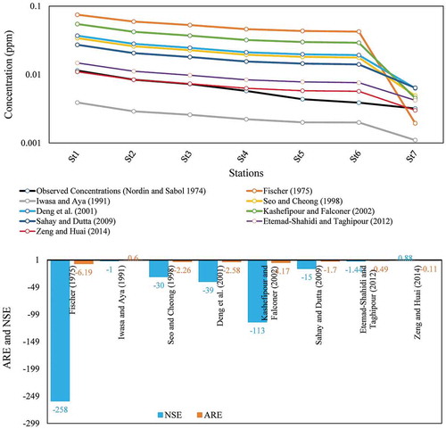
The Chattahoochee River is an important river in the southeast USA which supplies water for the Atlanta metropolitan areas (Tsivoglou and Wallace 1972). Nordin and Sabol (1974) conducted a tracer study by injection of dye material (mass: 7813 g) to the upstream of the river under IPL conditions. The peak concentration was detected at seven sampling sites, located about 16–76 km downstream of the injection point, revealing a mean velocity of 0.7 m s⁻¹ between the measurement stations (Atkinson and Davis 2000). The results of the measured concentrations at the stations are presented in Table 3.

2.4.3 River Severn

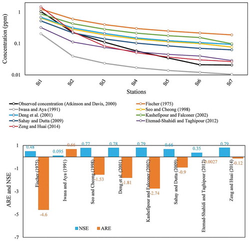
The River Severn, Britain’s longest river, is about 354 km long. Atkinson and Davis (2000) considered a reach of about 14 km of the river to study the pollution transport mechanism. Dye injection was carried out and water samples subsequently taken at seven downstream stations. The last sample was collected six and a half hours after discharging the material at the injection site. The results of the measured peak concentrations at different stations are presented in Table 3.

3 Results and discussion

No computational model can be used as a reliable tool unless its robust performance has been proved by numerous examinations. Hence, three extreme cases were considered: (a) comparison of the numerical results with analytical solutions; (b) model implementation under specific conditions (pure advection, advection–reaction and advection–dispersion–reaction); and (c) model performance in real case studies (i.e. the Athabasca, Chattahoochee and Severn rivers) under different scenarios in terms of different D_x estimation formulas.

3.1 Numerical vs analytical solution

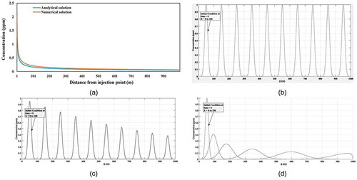
A comparison was carried out between two alternative solutions (numerical vs analytical) for an instantaneous loading at a completely uniform flow through a rectangular straight channel with the following characteristics: channel length: 1000 m, width and flow depth: 1 m, ∆t = 1 s, ∆x = 1 m, Q = 1 m³ s⁻¹, α = 0.5, C₀ = 2.3 mg L⁻¹ and k = 0.12 d⁻¹. The results presented in Figure 4(a) illustrate a good agreement between the numerical and analytical solutions.

Figure 4. (a) Comparison between analytical solution and numerical solution results from the developed model, and model performance (b) considering pure advection situation, (c) with simultaneous advection and reaction and (d) under advection–dispersion reaction conditions.

3.2 Model implementation under specific conditions

To test the model accuracy under pure advection (k = 0 d⁻¹ and D_x = 0 m² s⁻¹), the model was used with an initial Gaussian distribution of concentration along 100 m river distance and maximum solute concentration of C = 1 mg L⁻¹ (Fig. 4(b)) within a 1000-m long prismatic channel. In this solution, α = 1, ∆t = 1 s, ∆x = 1 m, U = 1 m s⁻¹, so that the Courant number is one. Figure 4(b) shows the simulated results under pure advection conditions. As expected, the initial conditions have been transferred to the downstream without any changes in the Gaussian distribution of the solute cloud. As is known, advection causes “sliding” of the initial solute distribution by moving the concentration curve with the flow velocity. It does not change the initial distribution of the dissolved material at all. Hence, there is an acceptable conformity between the model outputs and the proven hypothesis regarding the solute transport under pure advection conditions.

Another scenario was simulated, in which the solute was under advection–reaction conditions (Fig. 4(c)), with k = 0.12 d⁻¹. Theoretically, given the mentioned condition, results are anticipated to show a gradual decrease in the peak concentration of solute, while the cloud is transferring downstream without any spreading in the Gaussian shape (D_x = 0 m² s⁻¹). According to the results presented in Figure 4(c), it is clear that the model results are valid.

Finally, the developed model was implemented under advection–reaction–dispersion conditions, with D_x = 83 m² s⁻¹. In this situation, a gradual decrease in peak solute concentration should be observed when the cloud is transferring downstream, with spreading in the Gaussian shape. Figure 4(d) depicts this situation.

3.3 Model performance in real cases

The developed model was applied to simulate the solute transport resulting from STLP in the Athabasca River, and IPL in both the Chattahoochee and Severn. Also in this step, the developed numerical model was evaluated regarding several D_x estimation formulas. Note that at t = 0 the concentration value of the tracer is zero along the river for all the following cases.

3.3.1 Test case 1: STPL in the Athabasca River

The developed model was implemented to simulate the solute transport in the Athabasca River under STPL conditions. A fixed conservative Rhodamine concentration of 2.3 × 10⁵ mg L⁻¹, with a constant rate of 1.3 × 10^–4 mg L⁻¹ s⁻¹ was gradually introduced in the upstream river over a period of 5 hours. To check the effect of D_x, the model was evaluated by comparison with eight different D_x estimation formulas, and the calculated D_x values for all stations along the river are given in Table 4. The calculated D_x values vary between 110 and 13 403 m² s⁻¹ (Table 4). While these formulas were developed based on the same parameters W, d, U and U*, the authors used different regression techniques to tune their models for D_x estimation. In addition, these formulas were not developed with the same dataset. Therefore, it is easy to understand that these formulas resulted in different D_x values, although they used the same hydraulic and geometric characteristics at the same section along the river. However, Figure 5 shows the model performance with different D_x formulas, where ∆x = 100 m and α = 0.5. The downstream Rhodamine concentration is considered to be equal to the nearest upstream grid concentration because the solute becomes well mixed in the vertical and transverse directions in far-fields from the equilibrium zone.

Table 3. Flow and tracer test data collected on the Chattahoochee and Severn rivers. Injected mass at the beginning of the river: 7813 and 1000, respectively. Dist.: distance from injection point.

Station	Dist. (km)	Flow (m^3/s)	Time (h)	Slope (1/10 000)	Depth (m)	Width (m)	Observed concentration (ppm)
Chattahoochee River
St1	16	136	4.830	5.0	2.3	74.1	0.0114595
St2	27.9	180	8.080	2.8	2.9	65.8	0.0084092
St3	36.5	175	10.33	6.1	2.3	74.1	0.0072881
St4	49.6	170	14.80	3.1	2.3	77.7	0.0057677
St5	57.1	108	19.83	0.2	2.4	84.7	0.0043641
St6	60.5	108	21.50	4.4	2.4	84.7	0.0038850
St7	76.6	108	28.82	9.9	2.0	75.6	0.0031907
River Severn
St1	1.175	7	0.0833	142.8	0.462414	17.48697	1.0510314
St2	2.1	7	0.4333	51.81	0.385529	17.58157	0.2252745
St3	2.875	7	1.1333	11.76	0.572695	16.58974	0.1105359
St4	5.275	8	2.4667	16.67	0.621612	17.83409	0.0580027
St5	7.775	9	3.7333	24.00	0.527938	34.91049	0.0346054
St6	10.275	10	5.0333	44.00	0.423558	31.00417	0.0210800
St7	13.775	10	6.5369	25.71	0.624381	23.58682	0.0206550

Table 4. Comparison of D_x values for the Athabasca River calculated using different formulas.

Station	Dx estimation formula
	Fischer (1975)	Iwasa and Aya (1991)	Seo and Cheong (1998)	Deng et al. (2001)	Kashefipour and Falconer (2002)	Sahay and Dutta (2009)	Etemadshahidi and Taghipour (2012)	Zeng and Huai (2014)
St1	411	178	418	451	316	370	320	266
St2	595	173	488	515	388	431	337	269
St3	3341	362	614	524	307	724	364	290
St4	10994	506	795	520	332	1076	397	305
St5	861	311	407	442	209	444	320	279
St6	608	279	381	426	208	397	314	276
St7	13403	443	909	558	425	1183	411	302
St8	3146	467	525	464	213	675	348	294
St9	2740	348	587	522	299	679	360	289
St10	2040	389	498	476	228	594	343	289
St11	1756	402	460	454	202	555	333	287
St12	5138	594	552	442	192	778	354	301
St13	232	110	440	433	467	326	325	258
St14	1329	229	562	554	378	555	353	277
St15	1691	277	553	532	325	587	351	281
St16	1044	270	472	491	274	491	335	279
St17	5544	622	554	437	187	794	355	302
St18	2463	345	563	512	285	649	353	287
St19	1822	325	522	503	272	586	346	284
St20	507	326	327	379	155	358	299	276
St21	2606	413	494	448	211	618	330	278
St22	1864	478	429	426	165	550	327	291
St23	3723	236	808	651	572	822	396	286
St24	1390	286	509	509	289	543	344	282
St25	2714	213	758	648	569	741	387	281

Figure 5. Comparison of measured and simulated Rhodamine concentrations along the Athabasca River, Canada.

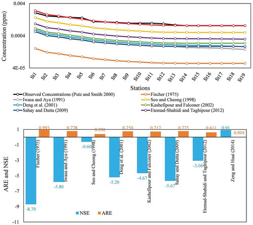
It was found that D_x has a great effect on the ADE performance. According to the results, the Zeng and Huai (2014) formula provides the best performance, with ARE and NSE of 0.004 and 0.909, respectively. Fischer’s (1975) formula resulted in the worst agreement with the measured values, as demonstrated by the ARE and NSE values of 0.993 and −8.7, respectively. The results support the conclusion drawn by Zeng and Huai (2014), who reported that most of equations underestimated D_x. However, Figure 5 indicates that, in the Zeng and Huai (2014) equation, there is some minor incompatibility between the simulated results and measured data (from injection point to station 13). This disagreement may be due to the effects of vertical and transverse mixing in the equilibrium zone. However, the model performance after the equilibrium zone (stations 14–18) is excellent. It is noted that when a solute resulting from a STPL is introduced into a river, the concentration in the far-fields of solute injection remains constant (Rutherford 1994). This situation occurs only after the equilibrium zone, where the solute becomes well mixed across the river. In other words, the concentration gradient of the solute in the longitudinal direction of the river becomes very small and negligible after the equilibrium zone. Consequently, it can be concluded that the developed model in combination with the Zeng and Huai (2014) formula appropriately supports the theoretical concepts and provides the best outputs compared to the measured data in the Athabasca River.

3.3.2 Test case 2: IPL in the Chattahoochee River

Similar to Test case 1, the developed model was evaluated using eight different D_x estimation formulas and data from the Chattahoochee River. Again ∆x = 500 m, α = 0.5, and the dye material is a conservative tracer, i.e. k = 0 d⁻¹. For the downstream boundary condition, it should be noted that the concentration at far downstream from Station 7 (St7) was considered equal to zero in any time step, as suggested by Chapra (1997).

Table 5 shows that the D_x values calculated with different formulas for stations 1–7 along the Chattahoochee River vary between 0.47 and 328 m² s⁻¹. Similar to the Test case 1, the different formulas resulted in different D_x values, although the same hydraulic and geometric characteristics are used in the formulas for the same section along the river. Figure 6 shows the simulated results from different D_x formulas at several downstream stations vs measured concentrations. The results indicate that when the model employs the Zeng and Huai (2014) formula, the best performance is achieved. The ARE and NSE are −0.11 and 0.88, respectively. There are considerable differences between the simulated results and field data on the Chattahoochee River for the Fischer (1975) formula (ARE: −6.19, NSE: −258).

Table 5. Comparison of D_x values for the Chattahoochee River calculated using different formulas.

Station	Dx estimation formula
	Fischer (1975)	Iwasa and Aya (1991)	Seo and Cheong (1998)	Deng et al. (2001)	Kashefipour and Falconer (2002)	Sahay and Dutta (2009)	Etemadshahidi and Taghipour (2012)	Zeng and Huai (2014)
St1	216	87	242	257	223	205	179	160
St2	177	54	282	279	328	204	184	172
St3	222	96	254	271	231	217	192	167
St4	308	73	280	288	278	231	180	167
St5	17	21	24	26	17	23	25	50
St6	0.47	100	2.81	1.52	1.21	4.32	13	26
St7	5.9	126	17	15	8.59	22	40	53

Figure 6. Comparison of measured and simulated solute concentrations along the Chattahoochee River, USA.

3.3.3 Test case 3: IPL in the River Severn

The model was run for the River Severn, with ∆x = 100 m, α = 0.5, and the dye material was conservative. The D_x values calculated with different formulas for all stations vary between 1.77 and 71 m² s⁻¹ (Table 6). Similar to Test cases 1 and 2, the use of different formulas resulted in different D_x values at all stations along the river. The downstream boundary condition is the same as that in the previous case. Figure 7 displays the model performance for this test case. Again, the results indicate that the Zeng and Huai (2014) formula achieved the best performance, with ARE and NSE values of −0.12 and 0.79, respectively. Also, the worst performance of the model was again obtained with Fischer’s (1975) equation (ARE: −4.6, NSE: 0.48).

Table 6. Comparison of D_x values for the River Severn calculated using different formulas.

Station	Dx estimation formulas
	Fischer (1975)	Iwasa and Aya (1991)	Seo and Cheong (1998)	Deng et al. (2001)	Kashefipour and Falconer (2002)	Sahay and Dutta (2009)	Etemadshahidi and Taghipour (2012)	Zeng and Huai (2014)
St1	14	53	25	28	15	27	36	22
St2	25	33	25	30	17	27	28	18
St3	12	14	20	21	16	18	20	17
St4	4.22	19	11	10	7.16	11	16	15
St5	8.0	62	8.60	11	4.17	13	17	17
St6	3.56	71	4.41	5.70	1.96	7.27	11	12
St7	1.77	35	5.0	4.58	2.54	6.37	12	12

Figure 7. Comparison of measured and simulated solute concentrations along the River Severn, UK.

4 Conclusions

In this study a numerical model was developed for simulating the solute transport of instantaneous and step loadings in rivers by solving the advection–dispersion equation (ADE). An integrated numerical code was developed using MATLAB and MS Excel as a user-friendly interface. Tracer study data in the Athabasca River (Canada), Chattahoochee River (USA) and River Severn (UK) were used. The most important findings of the research can be summarized as follows:

• The dispersion coefficient D_x estimated with the Zeng and Huai (2014) and Fischer (1975) formulas achieved, respectively, the best and worst performance in terms of agreement with the ADE results in all three case studies.

• Due to the effects of vertical and transverse mixing in the equilibrium zone, there were some discrepancies between the simulated results for the selected model that incorporates the Zeng and Huai (2014) equation for D_x estimation and the measured data in the Athabasca River. However, the selected model performance downstream of the equilibrium zone was excellent.

• The proposed numerical scheme in the developed water quality model showed that it was capable of accurately predicting tracer concentrations in 1D natural channels such that the simulated tracer concentrations were close to the observed data for all three case studies.

• The results of this study may be useful for water quality modelling where the RWQ models usually apply the proposed Fischer equation for determining D_x in ADE solutions. Meanwhile, incorporating the newly proposed equations for D_x estimation could improve the accuracy of ADE results.

• It is worth noting that the model was run for each river under the same conditions, except for the use of different D_x formulas. Therefore, the other error sources (e.g. accuracy of the hydraulic calibration, the restrictive Fickian assumption, the limited mixing downstream of inputs and through multi-channel systems) are the same for all scenarios of the ADE solution. Further studies on the effects of the other error sources on the ADE solution are needed, but were not within the scope of the present research.

• By linking the MATLAB software to MS Excel, the developed model provides a user-friendly platform for researchers. It is easy to use and applicable for RWQ modelling.

Disclosure statement

No potential conflict of interest was reported by the authors.

References

- Alizadeh, M.J., et al., 2017a. Prediction of longitudinal dispersion coefficient in natural rivers using a cluster-based Bayesian network. Environmental Earth Sciences, 76 (2), 86. doi:10.1007/s12665-016-6379-6
- Alizadeh, M.J., Ahmadyar, D., and Afghantoloee, A., 2017b. Improvement on the existing equations for predicting longitudinal dispersion coefficient. Water Resources Management, 31 (6), 1777–1794. doi:10.1007/s11269-017-1611-z
- Atkinson, T.C. and Davis, P.M., 2000. Longitudinal dispersion in natural channels: 1. Experimental results from the River Severn, U.K. Hydrology and Earth System Sciences, 4 (3), 345–353. doi:10.5194/hess-4-373-2000
- Balf, M.R., et al., 2018. Evolutionary polynomial regression approach to predict longitudinal dispersion coefficient in rivers. Journal of Water Supply: Research and Technology-Aqua, 67 (5), 447–457. doi:10.2166/aqua.2018.021
- Chapra, S.C., 1997. Surface Water-Quality Modeling. New York: Waveland Press.
- Chapra, S.C., Pelletier, G.J., and Tao, H., 2003. QUAL2K: A modeling framework for simulating river and stream water quality: documentation and user’s manual. Medford, MA: Civil and Environmental Engineering Department, Tufts University.
- Chow, V.T., 1973. Open Channel Hydraulics. New York: McGraw-Hill Company.
- Deng, Z., et al., 2002. Longitudinal dispersion coefficient in single-channel streams. Journal of Hydraulic Engineering, 128 (10), 901–916. doi:10.1061/(ASCE)0733-9429(2002)128:10(901)
- Deng, Z., Singh, V.P., and Bengtsson, L., 2001. Longitudinal dispersion coefficient in straight rivers. Journal of Hydraulic Engineering, 127 (11), 919–927. doi:10.1061/(ASCE)0733-9429(2001)127:11(919)
- Di Toro, D.M., Fitzpatrick, J.J., and Thomann, R.V., 1983. Water Quality Analysis Simulation Program (WASP) and Model Verification Program (MVP)-Documentation. Westwood, NY: Hydroscience, Inc., for US EPA, Duluth, MN. Contract, (68-01), 3872.
- El Kadi Abderrezzak, K., Ata, R., and Zaoui, F., 2015. One-dimensional numerical modelling of solute transport in streams the role of longitudinal dispersion coefficient. Journal of Hydrology, 527, 978–989. doi:10.1016/j.jhydrol.2015.05.061
- Etemadshahidi, A. and Taghipour, M., 2012. Predicting longitudinal dispersion coefficient in natural streams using M5′ model tree. Journal of Hydraulic Engineering, 138 (6), 542–554. doi:10.1061/(ASCE)HY.1943-7900.0000550
- Fischer, B.H., et al., 1979. Mixing in Inland and Coastal Waters. New York: Academic Press, Inc..
- Fischer, H.B., 1975. Discussion of “Simple method for predicting dispersion in streams”. Journal of Environmental Engineering Division - ASCE, 101 (3), 453–455.
- Ghane, A., Mazaheri, M., and Samani, J.M.V., 2016. Location and release time identification of pollution point source in river networks based on the Backward Probability Method. Journal of Environmental Management, 180, 164–171. doi:10.1016/j.jenvman.2016.05.015
- Goutal, N., et al., 2012, October. MASCARET: a 1D open-source software for flow hydrodynamic and water quality in open channel networks. In: R. Murillo Munoz, ed. River flow (Vol. 1). London: Taylor & Francis Group, 1169–1174.
- Haghiabi, A.H., 2016. Prediction of longitudinal dispersion coefficient using multivariate adaptive regression splines. Journal of Earth System Science, 125 (5), 985–995. doi:10.1007/s12040-016-0708-8
- Havnø, K., Madsen, M.N., and Dørge, J., 1995. MIKE 11–a generalized river modelling package. In: VJ. Singh, ed. Computer models of watershed hydrology. 733–782.
- Iwasa, Y. and Aya, S., 1991. Predicting longitudinal dispersion coefficient in open-channel flows. In: J. Lee and Y. Cheung, ed. Proceeding of International Symposium on Environmental Hydraulics. Hong Kong: International Association for Hydro-Environment Engineering and Research, 505–510.
- Kashefipour, M.S. and Falconer, R.A., 2002. Longitudinal dispersion coefficients in natural channels. Water Research, 36 (6), 1596–1608. doi:10.1016/S0043-1354(01)00351-7
- Nash, J.E. and Sutcliffe, J.V., 1970. River flow forecasting through conceptual models part I – A discussion of principles. Journal of Hydrology, 10 (3), 282–290. doi:10.1016/0022-1694(70)90255-6
- Noori, R., et al., 2019. A critical review on the application of the National Sanitation Foundation Water Quality Index. Environmental Pollution, 244, 575–587. doi:10.1016/j.envpol.2018.10.076
- Noori, R., et al., 2016. How reliable are ANN, ANFIS, and SVM techniques for predicting longitudinal dispersion coefficient in natural rivers? Journal of Hydraulic Engineering, 142, 4015039. doi:10.1061/(ASCE)HY.1943-7900.0001062
- Noori, R., et al., 2017. Estimation of the dispersion coefficient in natural rivers using a granular computing model. Journal of Hydraulic Engineering, 143, 4017001. doi:10.1061/(ASCE)HY.1943-7900.0001276
- Nordin, C.F. and Sabol, G.V., 1974. Empirical data on longitudinal dispersion in rivers. USA: US Geological Survey, Water-Resources Investigations, Report USGS/74-20.
- Park, S.S. and Lee, Y.S., 2001. A water quality modeling study of the Nakdong River, Korea. Ecological Modelling, 152 (1), 65–75. doi:10.1016/S0304-3800(01)00489-6
- Parsaie, A. and Haghiabi, A.H., 2017a. Numerical routing of tracer concentrations in rivers with stagnant zones. Water Science and Technology: Water Supply, 17 (3), 825–834. doi:10.2166/ws.2016.175
- Parsaie, A. and Haghiabi, A.H., 2017b. Computational modeling of pollution transmission in rivers. Applied Water Science, 7 (3), 1213–1222. doi:10.1007/s13201-015-0319-6
- Putz, G. and Smith, D.W., 2000. Two-dimensional modelling of effluent mixing in the Athabasca River downstream of Weldwood of Canada Ltd., Hinton, Alberta: development and verification of a two-dimensional hydraulic and kinetic model for the prediction of effluent transport in rivers. Edmonton: Sustainable Forest Management Network, Report2000-7/ERA.
- Rauch, W., et al., 1998. River water quality modelling: I. State of the art. Water Science and Technology, 38 (11), 237–244. doi:10.1016/S0273-1223(98)00660-X
- Rutherford, J., 1994. River Mixing. UK: John Wiley & Son Ltd., Chichester.
- Sahay, R.R. and Dutta, S., 2009. Prediction of longitudinal dispersion coefficients in natural rivers using genetic algorithm. Hydrology Research, 40 (6), 544–552. doi:10.2166/nh.2009.014
- Sattar, A.M.A. and Gharabaghi, B., 2015. Gene expression models for prediction of longitudinal dispersion coefficient in streams. Journal of Hydrology, 524, 587–596. doi:10.1016/j.jhydrol.2015.03.016
- Seo, I.W. and Cheong, T.S., 1998. Predicting longitudinal dispersion coefficient in natural streams. Journal of Hydraulic Engineering, 124 (1), 25–32. doi:10.1061/(ASCE)0733-9429(1998)124:1(25)
- Shakibaeinia, A., et al., 2016. An integrated numerical framework for water quality modelling in cold-region rivers: a case of the lower Athabasca River. Science of the Total Environment, 569-570, 634–646. doi:10.1016/j.scitotenv.2016.06.151
- Szymkiewicz, R., 2010. Numerical Modeling in Open Channel Hydraulics. New York: Springer.
- Tsivoglou, E.C. and Wallace, J.R., 1972. Characterization of stream reaeration capacity. USA: Office of Research and Monitoring, U.S. Environmental Protection Agency, Report-R3-72-012/EPA.
- USACE (US Army Corps of Engineers), 1986. HEC-RAS river analysis system.
- Zeng, Y. and Huai, W., 2014. Estimation of longitudinal dispersion coefficient in rivers. Journal of Hydro-Environment Research, 8 (1), 2–8. doi:10.1016/j.jher.2013.02.005