Performance evaluation of AR5-CMIP5 models for the representation of seasonal and multi-annual variability of precipitation in Brazilian hydropower sector basins under RCP8.5 scenario

ABSTRACT

Representations of precipitation from CMIP5 models over the 1950–1999 period in hydrographic basins that are relevant to the Brazilian electricity sector are evaluated in this study. The majority of ensemble members adequately represented seasonal variability, although they differed about the patterns of high-frequency interannual variation. The models did not adequately represent seasonal-scale precipitation in the southern region of Brazil. Relative to other models, the CNRM_CM5 and HadGEM2-ES models demonstrated good seasonal and interannual representation over most basins, while the global CanESM2, GFDL-ESM2M and IPSL_CM5A-LR models demonstrated relatively poor performance. The models concur on the impact of the RCP8.5 scenario in the Southeast/Midwest and South sectors over the period 2015–2044, suggesting that precipitation will decrease up to 15% in the basin supplying the Furnas hydropower plant and by 12% in the basin supplying the Itaipú plant, which represents 25% of the hydroelectric production in Brazil.

KEYWORDS:

• CMIP5 model
• hydroelectric sector
• climate change
• Brazil

Editor A. Castellarin Associate editor N. Ilich

1 Introduction

The Brazilian energy matrix has a very high level of clean energy, mostly due to high levels of hydroelectric production. Of the 116 618.4 MW authorized to the Brazilian electric sector, 68% is derived from hydroelectric power (ANEEL 2011). As a renewable energy source, hydropower offers significant advantages in terms of greenhouse gas emissions when compared to thermoelectric power generation, but it is sensitive to climate variables such as precipitation. Consequently, climate-informed management of hydropower in the Brazilian electric power matrix requires careful temporal variability analysis, considering the significant impact that variations in precipitation can have on the power supply and, consequently, on the national economy.

This has led to a high demand for climate information for decision-making at regional and local levels in both the public and private sectors. Accurate projections of climate change and climate variability are needed to improve the efficiency of energy planning and to minimize potential impacts on this resource availability (World Bank 2010).

Precipitation and streamflow projections provide important information for the hydroelectric sector by defining potential impacts on power generation. Further, the possibility to forecast climate change allows decision makers to prepare adaptation strategies, thus reducing the vulnerability of the Brazilian power supply. This information improves the understanding, sensitivity and limitations of these projections, making them tools for defining planning and management policies (Quiggin 2008, Van Vilet et al. 2012, 2016).

The basins of the Brazilian electricity sector are characterized by a climate with strong temporal and spatial variability of rainfall (Albuquerque et al., 2009). This complexity makes the region vulnerable to hydrological stress, and can lead to significant social and economic impacts in many sectors, such as during the “Brazilian electricity sector blackout” episode in 2001 (Watts and Ariztia 2002). Linking climate changes in the region to possible impacts on the flow regime is therefore a prerequisite to the development of optimal public policy.

Research on climate change and variability has focused on identifying the causes (Nobre 2005, IPCC 2007a), potential environmental, social and economic impacts (IPCC 2007b), and strategies to minimize the adverse consequences thereof. A particularly interesting branch of research is related to the efforts to identify the combination of planet temperature increases combined with changes in precipitation fields (Marengo and Soares 2005, Marengo and Valverde 2007).

The Intergovernmental Panel on Climate Change (IPCC) is a leading international scientific body on climate change assessments and its Fifth Assessment Report (AR5) reiterates that the warming of the climate system is unequivocal, and since the 1950s, many of the observed changes are unprecedented over time periods of decades to millennia. Moreover, the AR5 report included findings such as the increase of the global average air and ocean temperatures, the widespread melting of snow and ice, and the rising global average sea level. In addition, the level of greenhouse gas (GHG) concentrations has been higher and the temperature of the Earth’s surface in each of the last three decades has been successively warmer than any previous decade since 1850. The AR5 also points out that several parts of the world will find it difficult to find sources of drinking water and that the Andean communities, which depend on seasonal icemelt, will be adversely affected if glaciers continue to melt at an accelerated rate. Another AR5 highlight is the acceleration of climate variability. This means that, in recent years, scientists have observed higher occurrence of extreme events such as extreme floods, prolonged droughts and intense storms.

Despite the significant developments in the knowledge of climate change assessment, there are still many uncertainties associated with the various climate forecasts or projection systems. Some examples are the adopted physical parameterizations, the numerical methods applied to discretize boundary conditions of differential equations, the carbon cycle, clouds and aerosols representation, and the behaviour of the atmosphere itself (Meehl et al. 2005, Soden, Held 2006, Hargreaves 2010, Qian et al. 2016), which is considered as a chaotic system (Lorenz 1965). The unknown trajectory of future GHG concentrations is another process that is inherently uncertain. In the fifth phase of the Coupled Model Intercomparison Project (CMIP5), this uncertainty was addressed primarily through ensemble methods (Hou et al. 2001, Silveira et al. 2013).

Given alarge number of models and their highly divergent projections, especially over the Northeast region of Brazil and the Amazon (Lázaro 2011, Silveira and Souza Filho 2013), an evaluation methodology is needed to help to identify models that adequately represent the precipitation in the river basins relevant to the Brazilian hydroelectric sector. This evaluation should consist of two aspects: first identification of the best models by arguing that better representation of the twentieth century would lead to a more coherent representation of the future, and secondly identification of the worst models in order to remove them from the future statistical analysis.

Silveira et al. (2011) evaluated how the models of the IPCC fourth assessment report (IPCC-AR4) represent the seasonality of rainfall in the twentieth century in the northern Northeast of Brazil and indicated that most of the models adequately represent the climate in the region. Lázaro (2011) evaluated how the IPCC-AR4 models represent the multi-annual variation patterns for the northern Northeast of Brazil using wavelet transform and found that nearly one-fifth of the global IPCC-AR4 models represent satisfactorily the interannual and, in some cases, lower-frequency variations.

Previous studies have addressed evaluating how climate models represent precipitation over South America (e.g. Vera et al. 2006, Jones and Carvalho 2013, Yin et al. 2013), with a focus on synoptic and mesoscale alpha systems (2000 km). Vera et al. (2006) showed that a subset of CMIP3 models hardly represent the spatial pattern of precipitation over southeastern Brazil. The precipitation maximum in the South Atlantic Convergence Zone (SACZ) region during the winter is not well represented. However, seasonal cycle features are captured over the northern sector of South America. The simulation ability of CMIP5 models was evaluated by Yin et al. (2013), who showed that some models still present dry bias for the Amazon region and overestimate rainfall in the Intertropical Convergence Zone (ITCZ) over northeast South America. Jones and Carvalho (2013) assessed, in a historical experiment, how CMIP5 models represent large-scale features of the South America Monsoon System (SAMS). The main results showed that some models have improved their representation of the SAMS relative to the corresponding CMIP3 models. In general, previous studies have focused on a large-scale or regional patterns of atmospheric systems, such as ITCZ, SACZ and cold fronts.

In this paper, we address the Brazilian hydropower sector with analysis of the main reservoirs of different subsystems. The new approach here is relevant due to the high dependence on Brazil’s supply of hydroelectricity both at present and for long-term investment. The aim of this study is to develop a methodology for evaluating the ability of CMIP5 models to predict the regime of future seasonal and interannual rainfall and to apply this to the basins of the Brazilian electricity sector.

2 Method

2.1 Study region

The Brazilian electricity sector consists of more than 200 hydroelectric plants and several thermoelectric plants throughout the country. The planning of the Brazilian electrical system (generation and transmission), the National Interconnected System (NIS), attempts to scale up the demand and supply of future electric power configurations in the country. To do so, it is necessary to measure future energy needs, as well as adjust the schedules of entry of new generation projects, among other things. These adjustments are made following criteria that aim to ensure energy supply and minimize investment and operating costs. Information that allows a greater understanding of the aspects that affect the energy generation can provide a greater knowledge about risk in the decision-making and make the system’s water and energy allocation more efficient.

Figure 1 shows the basins of the NIS. Other than the Santo Antonio Basin, they are fully contained within Brazil. The extensive system of electricity production and transmission in Brazil implies a great diversity of regions, which are under the climatic influences of various meteorological phenomena. Because of this, several basins have distinct seasonal behaviour (see Section 3.1). Due to differences in hydrological seasonality and to produce synergetic gains, the system is divided into four sectors: the Southeast/Midwest, South, North and Northeast. These are interconnected by an extensive transmission network that enables the transfer of energy surpluses enabling the optimization of supply stored in the reservoirs of hydroelectric plants.

Figure 1. Map of the Brazilian hydropower sector (NIS) basins studied.

The nature of the NIS requires a spatial and temporal coupling of the decisions made in its energy operation. In this work, the studied basins were selected for the main hydroelectric projects in the country.

The Northeast sector is formed by the Três Marias, Sobradinho and Xingó basins (Fig.1). The Brazilian Northeast region has a well-defined annual cycle of precipitation, in which two distinct periods predominate: the rainy season and the dry season. The rainy season is concentrated between December and July, and the main rainfall system is the ITCZ.

The North sector is formed by the Serra da Mesa, Lajeado, Tucuruí, Belo Monte, Teles Pires, São Luiz do Tapajós and Santo Antônio basins (Fig.1). The seasonality of the North region is practically coincident with that of the Northeast region: during the rainy season, the flows of Tucuruí are extremely high, indicating that part of the energy generated can be taken to another region. The main rainfall climate system influencing this region is the SACZ.

The Southeast/Midwest sector has the country’s largest demand and imports energy from other regions for most of the year. The Southeast region consists of the basins Emborcação, Nova Ponte, Itumbiana, São Simão, Furnas, Água Vermelha, Nova Avanhandava, Porto Primavera, Rosana and Santa Cecilia (Fig.1). This region is also heavily influenced by the SACZ.

The South sector is comprised of the Itaipu, Salto Caxias, Itá and Dona Francisca basins (Fig.1). This region has great storage variability, and the Southeast/Midwest sector is extremely dependent on this sector. The climatology of the South region is heavily influenced by the incursion of cold fronts from high latitudes.

2.2 Observational data

The observational database is the reference used to determine the capabilities of the IPCC models in the continent. A comparison between two observed rainfall datasets is made in order to choose the more reliable one regarding monthly rainfall variability and climatology over the main basins of the NIS. The CRU monthly rainfall product of the Climate Research Unit (University of East Anglia, UK) (New et al. 2001) and the GPCC product of the Global Precipitation Climatology Centre of the German weather service (Deutscher Wetterdienst, Germany) (Schneider et al. 2011) are considered in this study. Both CRU and GPCC datasets have a resolution of 0.5 × 0.5 degrees and are calculated using raingauge data without having removed the bias correction. The datasets cover the period 1950–1999.

2.3 CMIP5 models

The data from the CMIP5 are the results of climate model simulations at various research centres that contributed to the reports of the IPCC, and the details are presented in Table 1. The models were driven by the observed concentrations of greenhouse gases during the twentieth century. For each model, one member was considered.

Table 1. The CMIP5 models analysed in this study. The models are identified in some figures by the ID number in column 1.

ID	Models	Institution	Reference
1	ACCESS1-0	Commonwealth Scientific and Industrial Research Organization (CSIRO) and Bureau of Meteorology (BOM), Australia	Bi et al. (2013b), Dix et al. (2013)
2	ACCESS1-3
3	bcc-csm1-1	Beijing Climate Centre, China Meteorological Administration, China	Wu (2012), Xin et al. (2012, 2013)
4	bcc-csm1-1-m
5	BNU-ESM	College of Global Change and Earth System Science, Beijing Normal University, China	Dai et al. (2003, 2004)
6	CanESM2	Canadian Centre for Climate Modelling and Analysis, Canada	Arora et al. (2011), von Salzen et al. (2013)
7	CESM1-CAM5	Community Earth System Model Contributors, USA	Hurrell et al. (2013)
8	CMCC-CM	Centro Euro-Mediterraneo per i Cambiamenti Climatici, Italy	Fogli et al. (2009), Scoccimarro et al. (2011)
9	CMCC-CMS		Fogli et al. (2009)
10	CNRM-CM5	Centre National de Recherches Meteorologiques/Centre Europeen de Recherche et Formation Avancees en Calcul Scientifique, France	Voldoire et al. (2013)
11	CSIRO-Mk3-6–0	CSIRO in collaboration with Queensland Climate Change Centre of Excellence, Australia	Rotstayn et al. (2012)
12	GFDL-CM3	Geophysical Fluid Dynamics Laboratory – NOAA, USA	Delworth et al. (2006), Donner et al. (2011),
13	GFDL-ESM2G		Dunne et al. (2012, 2013)
14	GFDL-ESM2M
15	GISS-E2-H	NASA Goddard Institute for Space Studies, USA	Schmidt et al. (2006)
16	GISS-E2-H-CC
17	GISS-E2-R
18	GISS-E2-R-CC
19	HadGEM2-AO	National Institute of Meteorological Research/Korea Meteorological Administration, South Korea	Collins et al. (2011), Martin et al. (2011)
20	HadGEM2-CC	Met Office Hadley Centre, UK
21	HadGEM2-ES
22	inmcm4	Institute for Numerical Mathematics, Russian Academy of Sciences	Volodin et al. (2010)
23	IPSL-CM5A-LR	Institut Pierre-Simon Laplace, France	Dufresne et al. (2012)
24	IPSL-CM5A-MR
25	IPSL-CM5B-LR
26	MIROC-ESM	Japan Agency for Marine-Earth Science and Technology, Atmosphere and Ocean Research Institute (The University of Tokyo), and National Institute for Environmental Studies	Watanabe et al., 2011
27	MIROC-ESM-CHEM
28	MIROC5	Atmosphere and Ocean Research Institute (The University of Tokyo), National Institute for Environmental Studies, and Japan Agency for Marine-Earth Science and Technology	Watanabe et al., 2010
29	MPI-ESM-LR	Max Planck Institute for Meteorology, Germany	Stevens et al., 2012
30	MPI-ESM-MR
31	MRI-CGCM3	Meteorological Research Institute, Japan	Yukimoto et al., 2011; Yukimoto et al., 2012
32	NorESM1-M	Norwegian Climate Centre, Norway	Iversen et al., 2013

The scenario of the projection simulations analysed here follows the RCP8.5 protocol: Representative Concentration Pathways with a target radiative forcing of 8.5 W/m² in 2100. This possible future scenario is consistent with high energy intensity and high dependence on fossil fuels, besides a continuous growth in the population. The RCP8.5 scenario has heavy greenhouse gas emissions associated with slow technological development and no implementation of climate policies (Riahi et al. 2011).

2.4 Evaluation criteria

To identify the models that best represent the 20th-century patterns of variation, the seasonal evaluation proposed by Silveira et al. (2011) was adopted together with an adaptation of the multi-annual evaluation proposed by Lázaro (2011). The evaluation consists of three steps that analyse variation patterns of different scales: seasonal, inter-annual and inter-decadal. Rainfall variability from climate models is evaluated against the observed time series over the hydrological basins.

For seasonal evaluation (AVAL_s) of the models, the average monthly weather in the study area for all of the IPCC models was compared to the observations (CRU) based on the selected statistical indices. The purpose is to define the models that best represent each relevant basin.

The inter-annual evaluation (AVAL_i) is based on the wavelet transform (Torrence and Compo 1998), especially when comparing the overall spectrum of power variation of the observed and modelled series. Each evaluation is assigned 0 or 1, representing, respectively, the worst and the best model for all the indexes of that analysis. From the calculation of AVAL_s and AVAL_i of all models, a general index, AVAL_g, is suggested, obtained by the sum of the evaluation weighted by ${\gamma }_j$ (which has values between 0 and 1), as follows:

(1) ${\mathrm{A}\mathrm{V}\mathrm{A}\mathrm{L}}_{\mathrm{g}}=\sum _{j=1}{\gamma }_j.{\mathrm{A}\mathrm{V}\mathrm{A}\mathrm{L}}_{\mathrm{i}}$(1)

(2) $\sum _{j=1}^{j=N}{\gamma }_j=1$(2)

The weighting can be done according to the interests of the evaluator: assigning an equal value of γ_j for all evaluations results in the same weight for each assessment in the overall index; assigning different values to the three evaluations results in different weights in the overall analysis. The general assessment of the CMIP5 models follows the hierarchical method of equations (1) and (2).

The workflow of the model evaluation is summarized in Figure 2. Seasonal assessment is performed by correlation analysis of the annual cycle and error analysis (equation (3)). Interannual assessment is performed by wavelet analysis based on a power spectrum of the time series between model and observation. The evaluation of the models is in the period 1950–1999.

Figure 2. Scheme of evaluation of the CMIP5 models for the period 1950–1999. All indexes are explained in the text.

2.4.1 Performance evaluation criteria for seasonality

We have used monthly precipitation as an evaluation criterion for seasonal representation of regional climate. Seasonal representation is highly relevant to assessing climate impact on water resources and agriculture. The beginning of crop cultivation and river regimes depends on how rainfall is distributed over time. Unsatisfactory representation of seasonality compromises the assessment of the impact of climate changes on those two important areas. Additionally, one can consider that monthly precipitation totals and their seasonality are an indication of the ability of the model to represent rain-generating systems and their occurrence.

To assess the models, we obtained the monthly mean climatological data of the studied region for all IPCC models and the historical observations (CRU continent and GPCC, no interpolation). Next, we compared models based on statistical indices to determine which models are most appropriate for northern Northeast Brazil.

The statistical measures used, as defined below, are: the root mean square error of the monthly percentage contribution concerning annual rainfall (RMSE) and correlation (CORREL) (Wilks 1995). The percentage RMSE (RMSE_PC) is the square root of the individual squared differences in means between the monthly percentage contribution of modelled rainfall in annual totals and the monthly percentage contribution of observed rainfall in annual totals, and is defined as:

(3) $\mathrm{R}\mathrm{M}\mathrm{S}{\mathrm{E}}_{\mathrm{P}\mathrm{C}}=\sqrt{\frac{1}{n}\sum _{i=1}^n{\left(\frac{100P_i}{{\sum }_{j=1}^n{P}_j}-\frac{100A_i}{{\sum }_{j=1}^n{A}_j}\right)}^2}$(3)

where n is the number of months, P is the CMIP5 model precipitation output for each month and the A is the observed value.

High values of RMSE_PC represent greater errors in forecast fields and values approaching zero point to a nearly perfect forecast. By squaring the difference term, the RMSE_PC tends to give more weight to the largest discrepancies between the observed and forecast fields.

The correlation can have values between – 1 and 1, which indicate, respectively, a perfect anti-correlation and perfect correlation; there is also the total lack of correlation which is determined when the result equals zero. The CORREL index can detect a phase correspondence between the time series:

(4) $\mathrm{C}\mathrm{O}\mathrm{R}\mathrm{R}\mathrm{E}\mathrm{L}=\frac{{\sum }_{i=1}^n\left(A_i-\bar{A}\right)\left(P_i-\bar{P}\right)}{\sqrt{{\sum }_{i=1}^n{\left(P_i-\bar{P}\right)}^2{\sum }_{i=1}^n{\left(A_i-\bar{A}\right)}^2}}$(4)

After calculating those two indexes, a weighted assessment is made so that the models can be ranked. This assessment is given by:

(5) $\mathrm{A}\mathrm{V}\mathrm{A}{\mathrm{L}}_{\mathrm{s}}={\alpha }_c\left(\frac{\mathrm{C}\mathrm{O}\mathrm{R}\mathrm{R}\mathrm{E}\mathrm{L}-\mathrm{C}\mathrm{O}\mathrm{R}\mathrm{R}\mathrm{E}{\mathrm{L}}_{\mathrm{m}\mathrm{i}\mathrm{n}}}{\mathrm{C}\mathrm{O}\mathrm{R}\mathrm{R}\mathrm{E}{\mathrm{L}}_{\mathrm{m}\mathrm{a}\mathrm{x}}-\mathrm{C}\mathrm{O}\mathrm{R}\mathrm{R}\mathrm{E}{\mathrm{L}}_{\mathrm{m}\mathrm{i}\mathrm{n}}}\right)+{\alpha }_r\left(\frac{\mathrm{R}\mathrm{M}\mathrm{S}{\mathrm{E}}_{\mathrm{P}\mathrm{C}\mathrm{m}\mathrm{a}\mathrm{x}}-\mathrm{R}\mathrm{M}\mathrm{S}{\mathrm{E}}_{\mathrm{P}\mathrm{C}}}{\mathrm{R}\mathrm{M}\mathrm{S}{\mathrm{E}}_{\mathrm{P}\mathrm{C}\mathrm{m}\mathrm{a}\mathrm{x}}-\mathrm{R}\mathrm{M}\mathrm{S}{\mathrm{E}}_{\mathrm{P}\mathrm{C}\mathrm{m}\mathrm{i}\mathrm{n}}}\right)$(5)

(6) ${\alpha }_c+{\alpha }_r=1$(6)

The choice of the coefficients ${\alpha }_c$ and ${\alpha }_r$ is based on the relevance of correlation and error, weighting the evaluation against the metrics.

The index CORREL_min is the smallest correlation obtained between the IPCC models and CORREL_max is the maximum correlation. Additionally, RMSE_PCmax is the maximum mean square percentage error of the IPCC models and RMSE_PCmin is the minimum.

The variables α_c and α_r have values between 0 and 1 (according to equation (6)), for α_c > α_r; therefore, the correlation has greater influence over the model assessment. However, for α_r > α_c the RMSE_PC of the models has greater weight in the assessment. When α_r= α_c = 0.5, the two metrics have the same weight on the AVAL_s value, and we considered α_r = α_c = 0.5 in this paper.

The AVAL_s variable has values between 0 and 1, which indicate, respectively, the worst and the best among the assessed models.

2.4.2 Performance assessment criteria of IPCC models – inter-annual variability

2.4.2.1 Time series analysis methods – wavelets

The wavelet term WT is defined in terms of a convolution integral between the analysed signal f(t) and a known wavelet function, expressed by:

(7) $\mathrm{C}\left(a,b\right)=\underset{-\mathrm{\infty }}{\overset{+\mathrm{\infty }}{\int }}\mathrm{f}\left(t\right){\psi }_{a,b}\left(t\right)\mathrm{d}t$(7)

in which parameters a and b vary continuously in R with a ≠ 0, and

(8) ${\psi }_{a,b}\left(t\right)=\frac{1}{\sqrt{a}}\psi \left(\frac{t-b}{a}\right)a\in R^{+}\mathrm{a}\mathrm{n}\mathrm{d}b\in R$(8)

The ψ_a,b functions are called daughter wavelets and are generated from dilations and translations of the mother wavelets ψ(t). The Morlet wavelet function was considered for analysis and is represented by:

(9) $\psi \left(t\right)={\pi }^{-1/4}{\mathrm{e}}^{i{w}_0\eta }{\mathrm{e}}^{-{\eta }^2/2}\mathrm{w}\mathrm{i}\mathrm{t}\mathrm{h}{w}_0=6\mathrm{a}\mathrm{n}\mathrm{d}\eta =t/s$(9)

where t is the time and s is the wavelet scale. This is a complex function and has features similar to those of the analysed time series, such as symmetry or asymmetry, and abrupt or soft time variation. The algorithm used was that developed by Torrence and Compo (1998).

2.4.2.2. Evaluation criteria

To evaluate the models, the global annual precipitation spectra are calculated for the studied regions in all CMIP5 models and the observations (CRU/GPCC). A comparison is made between the CRU spectrum regions having significance higher than 95% with the same spectral region of rounds of CMIP5 models.

The statistical measures used are correlation between power spectrums (CORREL) (equation (4)) and the distance of the variance variability of the simulations (DIST). Assuming the ratio between significant spectral variance and global spectrum variance of annual rainfall time series f_P and f_A, such that:

(10) $f_p=\frac{\mathrm{V}{\mathrm{P}}_s}{\mathrm{V}{\mathrm{P}}_G}\mathrm{a}\mathrm{n}\mathrm{d}{f}_a=\frac{\mathrm{V}{\mathrm{A}}_s}{\mathrm{V}{\mathrm{A}}_G}$(10)

where VP_s is the variance of the “predicted” precipitation in the wavelet spectrum significant region, VP_G is the variance of the entire global spectrum of the modelled power series, VA_s is the variance analysis of a significant region, and VA_G is the variance of the overall spectrum of wavelets of the observed data.

The Euclidean distance (DIST) indicates the variability of the variances of the runs of the models. It is related to the variance of observed data for bands and is defined by:

(11) $\mathrm{D}\mathrm{I}\mathrm{S}{\mathrm{T}}^2={\left(f_p-f_a\right)}^2$(11)

Large values indicate a greater distance DIST between the variances of the models and the variance of observed data.

After calculation of these indices, a weighted evaluation is made for the inter-representation, defined by:

(12) $\mathrm{A}\mathrm{V}\mathrm{A}{\mathrm{L}}_{\mathrm{i}}={\beta }_c\left(\frac{\mathrm{C}\mathrm{O}\mathrm{R}\mathrm{R}\mathrm{E}\mathrm{L}-\mathrm{C}\mathrm{O}\mathrm{R}\mathrm{R}\mathrm{E}{\mathrm{L}}_{\mathrm{m}\mathrm{i}\mathrm{n}}}{\mathrm{C}\mathrm{O}\mathrm{R}\mathrm{R}\mathrm{E}{\mathrm{L}}_{\mathrm{m}\mathrm{a}\mathrm{x}}-\mathrm{C}\mathrm{O}\mathrm{R}\mathrm{R}\mathrm{E}{\mathrm{L}}_{\mathrm{m}\mathrm{i}\mathrm{n}}}\right)+{\beta }_d\left(\frac{\mathrm{D}\mathrm{I}\mathrm{S}{\mathrm{T}}_{\mathrm{m}\mathrm{a}\mathrm{x}}-\mathrm{D}\mathrm{I}\mathrm{S}\mathrm{T}}{\mathrm{D}\mathrm{I}\mathrm{S}{\mathrm{T}}_{\mathrm{m}\mathrm{a}\mathrm{x}}-\mathrm{D}\mathrm{I}\mathrm{S}{\mathrm{T}}_{\mathrm{m}\mathrm{i}\mathrm{n}}}\right)$(12)

with

(13) ${\beta }_c+{\beta }_d=1$(13)

where DIST_max is the maximum distance of variabilities in the bands of model rounds and DIST_min is the minimum distance.

Variables β_c and β_r have values between 0 and 1 (according to equation (12)). For values β_c > β_r, the correlation has greater influence over the model assessment, while for β_c < β_r the distance between model variabilities has greater weight in the assessment. For β_c = β_r = 0.5 the two metrics have the same effect over the AVAL_i value. The AVAL_i variable has values between 0 and 1 which indicate, respectively, the worst and best among the assessed models.

2.5 Analysis of projections

For the calculation of seasonal anomalies, projections provided by global CMIP5 models for the RCP8.5 scenario for the period 2010–2099 are considered. A comparison is made with the models of the twentieth century for the period 1984–2003. In this analysis, only the models that pass the evaluation criteria are considered. To calculate the anomaly in the annual average, we use the following equation:

(14) $A_{\mathrm{a}\mathrm{n}\mathrm{n}\mathrm{u}\mathrm{a}\mathrm{l}}=\frac{P_{\mathrm{X}\mathrm{X}\mathrm{I}}^a-P_{\mathrm{X}\mathrm{X}}^a}{P_{\mathrm{X}\mathrm{X}}^a}\times 100$(14)

where $P_{\mathrm{X}\mathrm{X}\mathrm{I}}^a$ and $P_{\mathrm{X}\mathrm{X}}^a$ are the average annual rainfall for the scenarios of the twenty-first and twentieth centuries, respectively.

3 Results and discussion

3.1 Observed data

As mentioned, Brazilian river basins exhibit high spatial and temporal variation of rainfall. Distinctly different amounts of annual precipitation occur in similar basins at the same latitudes; for instance, as shown in Figure 3, São Luiz de Tapajós basin (23 in Fig.1) has an average annual rainfall of 2000 mm and that of Xingó basin (17 in Fig.1) is 500 mm/year.

A comparison of the annual precipitation of 24 basins from GPCC and CRU data for the period 1950–1999 is shown in Figure 3. The average long-term mean annual rainfall from the two datasets in each basin is quite similar; however, the GPCC shows higher coefficients of variation¹ in almost all catchments (Fig.3(b)). This is highlighted in Teles Pires, São Luíz do Tapajós, Tucuruí, and Belo Monte basins (North of Brazil), and in the Southeast region, for Embarcação, Nova Ponte and Itumbiara basins, as well as Itaipú (South region), which presents the largest divergences. This aspect is essentially relevant when looking at the statistical distribution of annual events in the twentieth century, where the dataset might not satisfactorily represent the inter-annual variability of total precipitation over the basin.

Figure 3. Comparison between GPCC and CRU datasets of the basins in the NIS for (a) mean total annual rainfall and (b) coefficient of variation.

Monthly climatology and the evolution of annual precipitation in São Luiz do Tapajós basin for GPCC and CRU datasets are shown in Figure 4. The average annual mean is approximately the same (2000 mm); however, the variance of the series is quite different. The CRU data present values between 1900 and 2300 mm, while the GPCC data show a range of 1600–2500 mm (Fig.4(a)). During the austral summer (December–February), the peak of the rainy season is in January for the GPCC data, whereas it is March for CRU (Fig.4(b)). The rainfall variability in this basin is modulated by Amazon convection activity from November to March, where the peak precipitation occurs in January based on raingauge data (Figueroa and Nobre 1990, Marengo 1995), which agrees with the GPCC dataset.

Figure 4. (a) Annual precipitation time series and (b) monthly precipitation climatology over São Luiz do Tapajós basin.

The CRU data cannot capture the annual rainfall variability (Reboita et al. 2010) for some regions, as seen in Figures 3 and 4. The problem possibly comes from issues in data consistency and spatial coverage of the raingauge stations providing the data. Therefore, the GPCC dataset is selected as the observational dataset in this paper to evaluate the CMIP5 models.

3.2 Seasonal assessment

Figure 5 shows the precipitation of the three best and three worst CMIP5 models (according to the seasonal assessment proposed herein) and GPCC data for Furnas, Itaipú, Sobradinho and Tucurui basins (these four power plants are representative of power generation in each NIS subsystem) for the period 1950–1999. Most models adequately represent the annual precipitation cycle. However, the models differ in the amount of rainfall, especially during the rainy season. Additionally, the models show great difficulty in representing the seasonality of the Itaipú basin, particularly in the months of April, May and June.

Figure 5. Climatology in terms of precipitation (1950–1999) from six CMIP5 global models and GPCC data (dashed line) for the Furnas, Itaipú, Sobradinho and Tucuruí basins. The models are chosen according to the AVAL_s criterion. The three best and three worst models are shown.

The NorESM1_M model underestimates the precipitation in most of the assessed basins, which is evident for Furnas basin, where the annual rainfall average is more than 50% lower than the observed data. Further, this model presented the poorest performance in representing the seasonal variability of rainfall in southern Brazil.

The GFDL_ESM2G model shows phase errors in the annual rainfall distribution over most of the basins. In Itaipú, for instance, it overestimates rainfall between April and November and underestimates it in the other months.

In addition, the IPSL_CM5A-LR and IPSL_CM5A-MR models do not represent the seasonality of precipitation in Northern and Northeastern basins. These results indicate how hard it is for climate models to represent precipitation in regions that are predominantly convective. Better results rely on higher resolution and improvements in the cumulus parameterization (Alves et al. 2016).

The HadGEM-AO model was found to be one of the best regarding seasonal precipitation in most basins, in the Southeast, South and North regions of Brazil.

The highest (max) and lowest (min) scores obtained for the proposed statistical indexes in the evaluation of the CMIP5 models at the seasonal scale for the Brazilian electricity sector basins are shown in Table 2. The models indicate a good representation of the seasonal variation patterns, with a minimum correlation greater than 0.7 in almost all basins. For the Itá and Dona Francisca basins the models show lower correlations compared to basins in other regions, indicating that there is poor seasonal representation for these basins; this is possibly due to the spatial scale of the models, since these are the two basins with smallest areas, or it may be due to the poor seasonal representation of South Brazil.

Table 2. Values of the proposed statistical indices for the evaluation of the CMIP5 models at the seasonal scale for the Brazilian electricity sector (NIS) basins. Bold values of the Pearson correlation coefficient (CORREL) are not significant at the 95% level.

	CORREL			RMSE
Basin	Max	Med	Min	Max	Med	Min
Emborcação	0.992	0.974	0.874	5.177	1.699	0.912
Nova Ponte	0.995	0.980	0.908	4.301	1.437	0.764
Itumbiana	0.993	0.971	0.855	5.602	1.948	0.805
São Simão	0.997	0.975	0.885	5.192	1.896	0.491
Furnas	0.995	0.979	0.867	3.663	1.519	0.788
Água Vermelha	0.993	0.978	0.923	4.004	1.668	0.716
N. Avanhandava	0.989	0.967	0.868	4.273	1.930	0.814
Porto Primavera	0.965	0.939	0.744	5.663	2.849	1.251
Rosana	0.987	0.972	0.921	5.098	2.565	0.857
Itaipú	0.870	0.820	0.692	7.158	4.093	1.443
Santa Cecília	0.992	0.964	0.836	3.373	1.660	0.712
Salto Caxias	0.816	0.681	0.492	6.371	3.508	1.100
Itá	0.823	0.581	0.404	5.272	3.140	1.181
Dona Francisca	0.651	0.050	–0.401	6.302	3.731	1.498
Três Marias	0.997	0.979	0.872	4.085	1.520	0.596
Sobradinho	0.982	0.925	0.707	7.605	2.866	1.635
Xingó	0.978	0.926	0.797	6.318	3.715	1.549
Serra da Mesa	0.994	0.963	0.808	6.671	2.279	0.754
Lageado	0.993	0.958	0.774	7.354	2.762	0.831
Tucuruí	0.994	0.974	0.839	5.993	2.079	0.735
Belo Monte	0.989	0.963	0.760	5.209	1.921	1.043
Teles Pires	0.997	0.977	0.835	5.182	1.863	0.630
S. L. do Tapajós	0.996	0.972	0.713	4.525	1.747	0.515
Santo Antônio	0.997	0.983	0.928	3.780	1.626	0.404

The AVAL_s and the classification (CLAS) of the CMIP5 models for the main basins of the Brazilian electricity sector (Furnas, Itaipú, Sobradinho and Tucuruí), with α_c equal to 0.5, are shown in Table 3. Different members of the same global model set (see Table 1) show very similar results for all the basins when compared to other models.

Table 3. AVAL_s of the CMIP5 models tested for the Furnas, Itaipu, Sobradinho and Tucuruí basins.

Model	Basin
	Furnas	Itaipu	Sobradinho	Tucurui
ACCESS1-0	0.802	0.883	0.926	0.880
ACCESS1-3	0.967	0.747	0.921	0.824
bcc-csm1-1	0.850	0.591	0.993	0.947
bcc-csm1-1-m	0.803	0.544	0.995	0.719
BNU-ESM	0.951	0.576	0.923	0.923
CanESM2	0.877	0.780	0.607	0.655
CESM1-CAM5	0.986	0.653	0.790	0.950
CMCC-CM	0.517	0.660	0.655	0.809
CMCC-CMS	0.688	0.703	0.753	0.838
CNRM-CM5	0.857	0.863	0.800	0.991
CSIRO-Mk3-6–0	0.743	0.516	0.962	0.823
GFDL-CM3	0.605	0.395	0.276	0.461
GFDL-ESM2G	0.108	0.115	0.157	0.263
GFDL-ESM2M	0.307	0.117	0.291	0.359
GISS-E2-H	0.243	0.519	0.648	0.698
GISS-E2-H-CC	0.089	0.573	0.682	0.764
GISS-E2-R	0.818	0.633	0.689	0.636
GISS-E2-R-CC	0.799	0.652	0.680	0.657
HadGEM2-AO	0.979	0.973	0.971	1.000
HadGEM2-CC	0.851	0.734	0.940	0.943
HadGEM2-ES	0.864	0.929	0.869	0.922
inmcm4	0.796	0.406	0.499	0.715
IPSL-CM5A-LR	0.703	0.063	0.158	0.060
IPSL-CM5A-MR	0.608	0.000	0.000	0.000
IPSL-CM5B-LR	0.988	0.511	0.352	0.563
MIROC-ESM	0.777	0.644	0.862	0.722
MIROC-ESM-CHEM	0.772	0.632	0.843	0.717
MIROC5	0.947	0.781	0.997	0.876
MPI-ESM-LR	0.864	0.876	0.856	0.839
MPI-ESM-MR	0.821	0.909	0.908	0.811
MRI-CGCM3	0.917	0.564	0.736	0.857
NorESM1-M	0.126	0.466	0.816	0.783

The members of the IPSL_CM5A_MR global model presented the worst runs, with AVAL_s near to zero in Itaipú, Tucurui and Sobradinho basins. The GFDL-ESM2M model was the worst model in most basins, showing AVAL_s lower than most other models. This indicates that the IPSL_CM5A_MR and GFDL-ESM2M global models do not represent the seasonality of the Brazil electricity sector basins adequately.

The AVAL_s for members of the CNRM-CM5, HADGEM2-AO and HADGEM2-ES models was higher than 0.750 in almost every NIS sector (Table 3). In contrast, despite having AVAL_s greater than 0.85 in the Northeast sector, as shown for the Sobradinho basin (Table 3), the NorESM1_M and CSIRO-MK-3–6-0 models have difficulty in representing seasonality in the South sector (Itaipú basin).

The difficulties the climate models have in representing the annual precipitation cycle on land may be due to inconsistencies in computing the energy budget on the ocean (Wild et al. 2015), as well as issues in the atmosphere–ocean interactions, such as variation modes of sea-surface temperature (SST) anomalies in the Atlantic and Pacific oceans. Once the downward solar and thermal radiation response by the incoming energy into the Oceans has occurred, recurrent bias is found over the Atlantic warm pool motivated by a radiative effect due to misrepresentation of high clouds and lower clouds in the atmospheric component of the models (Liu et al. 2013). In addition, this bias has been documented by Amaya et al. (2017) as a driver for errors in surface wind and latent heat flux anomalies throughout the tropical Atlantic and also the evolution of Atlantic Meridional Mode events among CMIP5 models. Further, the existence of systematic bias in simulating meridional width in El Nino-Southern Oscillation (ENSO) events has been demonstrated (Zhang et al. 2013). The CMIP5 models produce erroneous changes in trade winds and an imbalance of cross-equatorial flow in northern South America (Wang and Fu 2002). Problems in representing physical and dynamical processes in ocean and atmosphere have decreased from CMIP3 to CMIP5 models; however, some problems, such as clouds, surface fluxes, etc., remain, although they no longer reduce the confidence in the suitability of the models for detection studies and quantitative projections (IPCC 2013).

3.3 Inter-annual evaluation

3.3.1 Wavelet analysis

The overall spectrum of the observed series and the best and worst models for Furnas, Itaipú, Sobradinho and Tucuruí basins are shown graphically in Figure 6. The series of Tucuruí shows a strong dependence of the low-frequency variability with a wider range of 3 to 5 years band and with a significance level greater than 95%. Although it estimates a lower power, the INMCM4 member efficiently represents the standard spectrum considered significant and still captures reasonably well other patterns of the global power spectrum from the observed series. Meanwhile, the GFDL_ESM2M member has a very small spectral variance because it does not give proper weight to the main variation pattern. For the Furnas basin, the global spectrum of wavelets shows three well-defined patterns of variation, in which the highest power is between 13 and 25 years. The INMCM4 member obtained the highest rating, while the HadGEM2_CC member obtained the worst, which is evident when analysing the entire spectrum and observing that the HadGEM2-CC gives a much larger variance than the observed for the second pattern of variation (between 6 and 12 years).

Figure 6. Global wavelet spectrum of the best and worst CMIP5 models for Furnas, Itaipu, Sobradinho and Tucuruí basins in comparison with GPCC data. “o” indicates the best model, while “$\gamma$” indicates the worst; $\gamma$ is the observation data.

In Itaipú basin, precipitations of the GPCC show a high participation of the high frequency in the variability of the time series. The ACCESS1-0 model represents the inter-annual variability and shows a very high spectral correlation within the region of the spectrum considered significant.

For the Sobradinho basin, although it did not present a good seasonal review, the GFDL-ESM2G member had the highest inter-annual review, showing a very high correlation between the significant part of the spectrum. Simultaneously the CSIRO-MK-3–6-0 member had the worst rating, due to its low correlation with the entire global spectrum of wavelets and for presenting a much greater variance to high-frequency variation.

Table 4 shows the highest and lowest values of statistics (correlation and distance) for the CMIP5 models evaluation on an inter-annual scale, considering the Brazil’s electricity sector basins. The models indicate large dispersion compared to the overall spectrum of wavelets observed with correlations and distances between extremely different variances.

Table 4. Best and worst values obtained from the proposed statistical indexes for the seasonal CMIP5 models evaluation on a inter-annual scale, considering the Brazilian electricity sector basins. Bold values of Pearson’s Correlation coefficient are not significant at 95%.

	CORREL			DIST
Basin	Max	Med	Min	Max	Med	Min
Emborcação	0.929	0.798	0.594	1.160	1.084	0.971
Nova Ponte	0.956	0.795	0.418	1.170	1.091	0.949
Itumbiana	0.939	0.747	0.499	1.200	1.111	1.012
São Simão	0.949	0.844	0.628	1.171	1.095	0.917
Furnas	0.937	0.808	0.423	1.187	0.096	0.925
Água Vermelha	0.957	0.855	0.661	1.167	1.085	0.959
Nova Avanhandava	0.919	0.835	0.654	1.121	1.045	0.968
Porto Primavera	0.910	0.745	0.413	1.140	1.059	0.905
Rosana	0.960	0.784	0.452	1.170	1.091	0.950
Itaipú	0.897	0.787	0.591	1.218	1.137	1.023
Santa Cecília	0.966	0.845	0.498	1.157	1.074	0.981
Salto Caxias	0.921	0.750	0.454	1.168	1.109	1.007
Itá	0.943	0.809	0.547	1.145	1.088	0.992
Dona Francisca	0.951	0.857	0.481	1.134	1.060	0.948
Três Marias	0.935	0.778	0.381	1.154	1.069	0.870
Sobradinho	0.940	0.635	0.293	1.199	1.118	1.008
Xingó	0.957	0.696	0.101	1.122	1.024	0.836
Serra da Mesa	0.942	0.783	0.470	1.193	1.103	0.975
Lageado	0.908	0.746	0.366	1.124	1.064	0.932
Tucuruí	0.939	0.747	0.348	1.155	1.036	0.872
Belo Monte	0.948	0.828	0.684	1.096	0.963	0.843
Teles Pires	0.967	0.801	0.571	1.108	0.989	0.877
São Luiz do Tapajós	0.971	0.811	0.586	1.068	0.919	0.758
Santo Antônio	0.976	0.592	0.390	0.974	0.906	0.828

The AVAL_i and a classification of the CMIP5 models for the main basins (Furnas, Itaipú, Sobradinho and Tucuruí) with βc equals to 0.5 are shown in Table 5. The different group members of the same global model show different results for most of the basins when compared to one another.

Table 5. AVAL_i of the CMIP5 models for the Furnas, Itaipú, Sobradinho and Tucuruí basins.

Model	Basin
	Furnas	Itaipu	Sobradinho	Tucurui
ACCESS1-0	0.615	0.811	0.371	0.386
ACCESS1-3	0.632	0.616	0.617	0.578
bcc-csm1-1	0.709	0.191	0.647	0.472
bcc-csm1-1-m	0.213	0.198	0.509	0.527
BNU-ESM	0.279	0.447	0.597	0.474
CanESM2	0.390	0.570	0.665	0.499
CESM1-CAM5	0.469	0.489	0.379	0.591
CMCC-CM	0.314	0.398	0.514	0.718
CMCC-CMS	0.496	0.776	0.453	0.630
CNRM-CM5	0.464	0.566	0.424	0.516
CSIRO-Mk3-6–0	0.693	0.366	0.234	0.436
GFDL-CM3	0.407	0.601	0.345	0.588
GFDL-ESM2G	0.351	0.443	0.862	0.743
GFDL-ESM2M	0.685	0.737	0.498	0.342
GISS-E2-H	0.454	0.272	0.327	0.553
GISS-E2-H-CC	0.410	0.348	0.485	0.783
GISS-E2-R	0.434	0.657	0.711	0.845
GISS-E2-R-CC	0.412	0.064	0.475	0.768
HadGEM2-AO	0.566	0.593	0.407	0.507
HadGEM2-CC	0.201	0.211	0.277	0.355
HadGEM2-ES	0.222	0.364	0.718	0.731
inmcm4	0.749	0.319	0.838	0.885
IPSL-CM5A-LR	0.547	0.503	0.858	0.714
IPSL-CM5A-MR	0.618	0.778	0.332	0.541
IPSL-CM5B-LR	0.686	0.311	0.342	0.507
MIROC-ESM	0.617	0.532	0.744	0.432
MIROC-ESM-CHEM	0.676	0.459	0.472	0.442
MIROC5	0.514	0.222	0.465	0.532
MPI-ESM-LR	0.538	0.792	0.310	0.539
MPI-ESM-MR	0.580	0.669	0.398	0.498
MRI-CGCM3	0.854	0.944	0.355	0.456
NorESM1-M	0.492	0.688	0.413	0.501

In Tucurui and Sobradinho, the INMCM4 run shows AVAL_i greater than 0.8, which indicates that the members of this global model represent well the annual growth cycle of high frequency on the observed data. Moreover, in Furnas the members of the HadGEM2-CC model have AVAL_i slightly lower than the most members of the set. Likewise, in Itaipú the GISS-E2-R-CC model also does not adequately represent the patterns of annual precipitation variation, with AVAL_i near to 0.1.

3.3.2. Taylor diagram

Most models have rainfall variability similar to the GPCC observational database, with the observed standard deviation for the Sobradinho hydrographic basin ranging between 0.5 and 1.5 (Fig.7(a)). This basin has an area of 448 217 km², providing a greater capacity of the models to capture the monthly variation of precipitation observed during the twentieth century; at least 80% of the models had time correlation above 0.6 for the period 1950–1999. This result suggests that global climate models with a spatial resolution of around 150 × 150 km are able to simulate precipitation variability over this basin. However, there are issues in the simulated series variance from some models. For example, the variability intensity presented by the NorESM1-M model is lower and the RMSE is 1 SD, as opposed to the IPSL-CM5B-LR and MIROC5 models, which are outside the envelope of 1.5 SD with a standard error of around 1.5.

Figure 7. Taylor diagrams for the Sobradinho, Tucuruí, Itaipu and Furnas hydrographic basins. The concentric arcs labelled REF represent the RMSE normalized by the standard deviation.

The extent of hydroeletric plants in the Tucuruí basin, located in the centre of Brazil, resembles that of the Sobradinho basin (Fig.1). In this basin, the precipitation was simulated with temporal coherence compared to the historical regime, and the models had good correlation to the GPCC dataset (Fig.7(b)). While the correlation of most of the models is above 0.8, the results match the variability of the observational data series, and the precipitation simulations have a standard deviation that is distributed around the observed value, without disaggregating with high values of RMSE.

The issue of obtaining more reasonable results from large hydrographic basins is related to the horizontal resolution of the global models. This was seen in the cases of the Itaipú and Furnas basins, with areas of 150 685 and 51 734 km², respectively. These basins are dramatically smaller than the Tucuruí and Sobradinho basins (see also Fig.1). It may be seen in Figure 7(c) that the models have greater difficulty to be precise for the Itaipú precipitation, with correlation values in the sector of between 0.2 and 0.4. These values are show less reliability, although valid results for the hydrographic region for the longest duration climate feature continue to be noticed, once discrepancy in terms of variance and RMSE does not compromise the ensemble models results.

For the watershed that discharges into the Furnas hydroelectric plant (Fig.7(d)), the models are not representative of the GPCC data in terms of the variance, for which the results show errors of SD between 0.5 and 0.75 (RSME > 1) for many of the models. The monthly variability was better captured; the correlation for rainfall estimation over the basin had values of between 0.6 and 0.8 for most of the simulations.

3.4 General assessment

The AVAL_g of the CMIP5 models for major basins in the Southeast/Midwest of the Brazilian electricity sector is shown in Figure 8. The members of the CNRM_CM5 global model present the best AVAL_g values, followed by the runs of the HadCM3 and HadGEM2-ES models. Meanwhile, the GFDL-ESM2M and IPSL_CM5A_LR global models are clearly inferior to the others, with AVAL_g values below 0.5.

Figure 8. Total AVAL_g of the major basins in the Southeast/Midwest of the Brazilian electricity sector (NIS).

In the same way, general assessment of the models shows good performance over most of the basins in the South region of Brazil (Fig.9(a)). The models show difficulty when representing the variability patterns of the basins in this sector, with most models indicating AVAL_g below 0.5. Members of the MRI_CGCM3, CNRM_CM5, HadCM3 and HadGEM2-ES global models have the best AVAL_g values, while global models CSIRO-MK-3–6-0, GFDL-ESM2M and IPSL_CM5A_LR clearly have poor performance, with AVAL_g lower than 0.5.

Figure 9. AVAL_g of the major basins in (a) the South, (b) the Northeast and (c) the North of the Brazilian electricity sector.

The AVAL_g of the CMIP5 models for major basins in the Northeast of the Brazilian electricity sector is shown in Figure 9(b). The runs of the CanESM2, GFDL_ESM2M and IPSL_CM5A_LR global models show lower AVAL_g than the others, with values that do not exceed 0.5. The runs of the GISS-E2-R and CNRM-CM5 models in the Xingó basin, gave the highest AVAL_g values, while for the Sobradinho basin the CSIRO-MK-3–6-0, HadCM3 and HadGEM2-ES models had better performance.

The AVAL_g of the CMIP5 models for major basins in the North of the Brazilian electricity sector is shown in Figure 9(c). The HadGEM2-ES_r1i1p1 member shows AVAL higher than 0.8 in all basins of the region.

3.5 Projections of the models

Figure 10 shows the comparison between the reference period (1984–2003) and projected 2015–2044, 2045–2074 and 2075–2098 periods in the Brazilian hydroelectricity sector basins using the RCP8.5 scenario. The medians of annual mean precipitation anomalies from global model projections indicate that the impact is not uniform throughout Brazil. The occurrence of more moist conditions is projected over southernmost Brazil at the end of twenty-first century, while other regions of the country will probably present reduced precipitation (Fig.10(a) and (b)).

Figure 10. Impact on the average annual rainfall in the twentieth century for CMIP5 models with a RCP8.5 scenario in relation to the reference period (1984–2003) for (a) 2015–2044; (b) 2045–2074 and (c) 2075–2098. The models with AVAL_g below 0.2 were removed from this analysis.

There is a light dispersion in the projections for the North sector, although most models pointed to a decrease in annual precipitation at the end of the twentieth century (Fig.10(c)). For Santo Antonio basin, the slight reduction indicates that there is a major influence on climate change in the tropical sector (São Luiz dos Tapajós, Teles Pires and Belo Monte basins).

For the Northeast sector, the models indicate significant uncertainty, with no convergence in the results (Silveira et al. 2013). In the Xingó basin, for example, the models show increased precipitation of up to 20% for the three periods. Yet, the models indicate reductions in precipitation of over 30% for all three periods.

On the Southeast/Midwest region of Brazil, the models show anomalies with different patterns in regions that respond differently to climate change, for instance, the most of centre-west region and the coastal region of the Southeast of the country. This is seen in Figure 10(b), which shows more intense negative anomalies in the Midwest of Brazil, in Emborcação, Nova Ponte and Itumbiara basins. Southeast Brazil is a region that presents a widespread projection of future changes in climate, with divergence among the models increasing from the beginning to the end of the century, most notably in Itá and Salto Caxias basins (Fig.10(a), (b) and (c)).

The seasonal changes demonstrated by the climate models are analysed based on anomalies departing from recent climate data. These anomalies are projected on the climatology of the annual cycle observed for each basin. The standard deviation between the projections is indicated in the grey shaded parts of Figure 11.

Figure 11. Seasonal projection (2070–2098 relative to 1984–2003) under the RCP8.5 scenario. The grey shaded area is computed by standard deviation anomaly of the models projected onto observational monthly precipitation for (a) Furnas, (b) Itaipú, (c) Sobradinho and (d) Tucuruí basins.

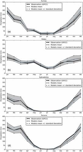
For Furnas basin, the models indicate a greater possibility of reduced rainfall at the beginning of the season (August and September), associated with a higher probability of an increase in other periods of the year. This characteristic can delay the recharge of reservoirs and requires a greater amount of water to be stored for a greater part of the year. This situation can have an impact on the generation of energy in this sector, since it depends on the streamflow regulated by the reservoirs (Fig.11(a)).

For Itaipú basin, an increase in annual precipitation is likely; however, in August and September, most of the models indicate a reduction in rainfall. This behaviour indicates that the precipitation climatology can be altered with greater contributions in the rainfall amount in April–July (Fig.11(b)).

Sobradinho (Northeast sector) and Tucuruí (North sector) basins have similar projection behaviour, showing decreasing precipitation through the demise and onset of the wet season (Fig.11(c) and (d)). In general, during peak of the rainy period present high uncertainty in the projections with widespread of the anomalies, this characteristic is emphasized in Sobradinho basin (Northeast sector) (Figure 11c).

4 Conclusions

The evaluation proposed in this study identified the best and worst models in the representation of the variation of the rainfall patterns in the twentieth century in the basins of the Brazilian hydroelectric sector. This information can be used by managers seeking the most likely projections for the twenty-first century and by scientists looking for a possible statistical treatment of all the projections. The latter group may use the results of this study to assess the impact on streamflow and evapotranspiration with the largest number of possible models for treating and sizing the existing uncertainty in climate projections.

The regional aspects of runoff can vary substantially based on surface land use and topography, which lead to problematic issues of modelling land processes in the inherent spatial and temporal scales in which they occur (Thomas and Sellers 1991). However, current improvements in the physical representation of surface–atmosphere interaction enable most global climate models to capture general features such as precipitation and evapotranspiration pattern (Pitman 2003; Flato et al. 2013). In fact, at the scale of large basins, the regional hydrology might not be relevant at the monthly timescale where the mean characteristics captured by the climate models take place.

As for the seasonal evaluation of CMIP5 models, some features are highlighted:

• Most IPCC-AR4 global models showed high correlation with respect to climatological precipitation in the period 1950–1999 for the evaluated areas, showing that the models are able to represent the patterns of seasonal variations.

• The IPSL_CM5A-LR and GFDL-ESM2M models did not adequately represent the average climatology of most basins in the electricity sector of Brazil.

• In general, the models did not accurately represent the seasonal cycle of precipitation over the south of the country, with lower correlation than basins in other domains.

• For the inter-annual evaluation of CMIP5 models, some features are highlighted: (i) the wavelet transform shows that there are variations at various time scales in the observed data for rainfall behaviour in the twentieth century, due to the random characteristic of large-scale circulation of the atmosphere (Lorentz 1975). This restricts the use of some CMIP5 models for some regions, as these models are approximate representations of a very complex system, and as shown in the results, some are not able to represent the random nature of precipitation in the twentieth century. (ii) Spectral analysis of the runs of CMIP5 models showed large differences in the representation of the inter-annual variability of rainfall in the basins. (iii) The runs of the CanESM2 model did not adequately represent the annual variation of rainfall patterns in most of the electricity sector basins.

For most basins, the runs of the CNRM_CM5 and HadGEM_ES models showed AVAL_g greater than 0.7, which indicates that for a possible dynamic downscaling in using a regional model they would be a good choice for the evaluation of the Brazilian electric sector. Due to the high computational cost demanded by this technique, the use of a large number of global models is limited.

The runs of CanESM2, GFDL-ESM2M and IPSL_CM5A-LR models are clearly inferior to the others, with AVAL_g below 0.5 in nearly all basins. This indicates that, for a possible analysis of the projections using the ensemble technique, these members can make the set noisy and divergent from future weather conditions, increasing the level of calculated uncertainty associated with projections of the set.

For the projections of the CMIP5 models analysed under the RCP8.5 scenario for the twentieth century, there are differences in the future precipitation in the different regions of the electricity sector. This scattering may be associated with uncertainty itself from meteorological phenomena involving precipitation – “the atmosphere is a chaotic system”, as stated by Lorenz (1965) – and/or misrepresentation of micro- and meso-scale phenomena that need to be resolved at a higher resolution.

In the South and Southeast/Midwest sectors, the models indicate margins suggesting a greater possibility of reductions in rainfall or a slight increase, but in the Northeast sector, there is greater uncertainty among models and there is no convergence regarding the results.

The CMIP5 models converge in their assessment of the impact on the electricity sector in the Southeast/Midwest and South sectors in the period 2015–2044, showing that precipitation is expected to reduce by up to 15% in Furnas basin and approximately 12% in Itaipu basin. This reduction suggests quite an impact on power generation in these sectors, which requires planning measures to minimize the possible losses if these projections are confirmed. For the North and Northeast sectors, the divergence between models indicates significant uncertainty, but suggests a margin in which the infrastructure planning should occur.

The divergences of the CMIP5 models analysed demonstrate a high level of uncertainty in their projections. However, this information defines a margin of possible future scenarios of rainfall in the Brazilian electricity sector and should be used for the adoption of policies and management.

Obviously, projections with less uncertainty would be more interesting for decision makers; however, this does not occur in regional projections of CMIP5 models, especially for smaller areas. Forcing the reduction of these uncertainties may induce strategies that lead to great regret, to borrow terminology from the risk management literature. Hence, robust strategies need to consider the uncertainties in the current level of knowledge.

Disclosure statement

No potential conflict of interest was reported by the authors.

Notes

¹ The coefficient of variation is defined as the ratio of the standard deviation to the mean.

References

- Alburquerque, I.F., et al., 2009. Tempo e Clima no Brasil. São Paulo:Oficina de Textos, 280.
- Alves, J., et al., 2016. Evaluation of the AR4 CMIP3 and the AR5 CMIP5 model and projections for precipitation in Northeast Brazil. Frontiers in Earth Science, 4.
- Amaya, D. J., et al., 2017. WES feedback and the Atlantic Meridional Mode: observations and CMIP5 comparisons. Climate Dynamics, 49 (5–6), 1665–1679.
- ANEEL. Banco de Geração de Informações – capacidade de Geração do Brasil. Available from: http://www.aneel.gov.br/aplicacoes/capacidadebrasil/capacidadebrasil.asp [Accessed 03 Apr 2011].
- Arora, V.K., et al., 2011. Carbon emission limits required to satisfy future representative concentration pathways of greenhouse gases. Geophysical Research Letters, 38, L05805. doi:10.1029/2010GL046270
- Bi, D., et al., 2013b. The ACCESS coupled model: description, control climate and evaluation. Australian Meteorological and Oceanographic Journal, 63, 41–64. doi:10.22499/2.6301.004
- Collins, W.J., et al., 2011. Development and evaluation of an earth-system model-HadGEM2. Geoscientific Model Development, 4, 1051–1075. doi:10.5194/gmd-4-1051-2011
- Costa, F.S., Maceira, M.E.P., and Damázio, J.M., 2007. Modelos de Previsão Hidrológica Aplicados ao Planejamento da Operação do Sistema Elétrico Brasileiro. RBRH, Revista Brasileira de Recursos Hídricos, 12 (3), 21–30. doi:10.21168/rbrh.v12n3.p21-30
- Dai, Y.J., et al., 2003. The common land model. Bulletin of the American Meteorological Society, 84, 1013–1023. doi:10.1175/BAMS-84-8-1013
- Dai, Y.J., Dickinson, R.E., and Wang, Y.P., 2004. A two-big-leaf model for canopy temperature, photosynthesis, and stomatal conductance. Journal of Climate, 17, 2281–2299. doi:10.1175/1520-0442(2004)017<2281:ATMFCT>2.0.CO;2
- Delworth, T.L., et al., 2006. GFDL’s CM2 global coupled climate models. Part I: formulation and simulation characteristics. Journal of Climate, 19, 643–674. doi:10.1175/JCLI3629.1
- Dix, M., et al., 2013. The ACCESS coupled model: documentation of core CMIP5 simulations and initial results. Australian Meteorological and Oceanographic Journal, 63, 83–99. doi:10.22499/2.6301.006
- Donner, L.J., et al., 2011. The dynamical core, physical parameterizations, and basic simulation characteristics of the atmospheric component AM3 of the GFDL global coupled model CM3. Journal of Climate, 24, 3484–3519. doi:10.1175/2011JCLI3955.1
- Dufresne, J.-L., et al., 2012. Climate change projections using the IPSL-CM5 earth system model: from CMIP3 to CMIP5. Climate Dynamics. doi:10.1007/s00382-012-1636-1
- Dunne, J.P., et al., 2012. GFDL’s ESM2 global coupled climate-carbon earth system models. Part I: physical formulation and baseline simulation characteristics. Journal of Climate, 25, 6646–6665. doi:10.1175/JCLI-D-11-00560.1
- Dunne, J.P., et al., 2013. GFDL’s ESM2 global coupled climate-carbon earth system models part II: carbon system formulation and baseline simulation characteristics. Journal of Climate. doi:10.1175/JCLI-D-12-00150.1
- Figueroa, S.N. and Nobre, C.A., 1990. Precipitation distribution over central and western tropical South America. CLIMANÁLISE- Boletim de Monitoramento e Análise Climática, 5 (6), 36–45.
- Flato, G., et al., 2013. Evaluation of climate models. In: Climate change 2013: the physical science basis. Contribution of working group I to the fifth assessment report of the intergovernmental panel on climate change. Climate Change, 5 (2013), 741–866. Cambrigde University Press.
- Fogli, P.G., et al.2009. INGV-CMCC carbon (ICC): a carbon cycle earth system model. CMCC Research Papers. Bologna, Italy: Euro-Mediterranean Centre on Climate Change, 31.
- Hargreaves, J.C., 2010. Skill and uncertainty in climate models. Wiley interdisciplinary reviews. Climate Change, 1 (4), 556–564.
- Hou, D., et al., 2001. Objective verification of the Samex’98 Ensemble forecast. Monthly Weather Review, 129, 73–91. doi:10.1175/1520-0493(2001)129<0073:OVOTSE>2.0.CO;2
- Hurrell, J., et al., 2013. The community earth system model: A framework for collaborative research. Bulletin of the American Meteorological Society. doi:10.1175/BAMS-D-12–00121
- IPCC (Intergovernmental Panel on Climate Change), 2007a. Climate change 2007: the physical science basis. Cambridge, UK: Cambridge University Press.
- IPCC (Intergovernmental Panel on Climate Change), 2007b. Climate change 2007: impacts, adaptation and vulnerability. Cambridge, UK: Cambridge University Press.
- IPCC (Intergovernmental Panel on Climate Change), 2013. Climate change 2013: the physical science basis. Contribution of working group I to the fifth assessment report of the intergovernmental panel on climate change [eds. T.F. Stocker, et al.]. Cambridge, UK and New York, NY: Cambridge University Press, 1535pp.
- Iversen, T., et al., 2013. The Norwegian earth system model, NorESM1–M. Part 2: climate response and scenario projections. Geoscience and Model Development, 6, 1–27.
- Jones, C. and Carvalho, L.M.V., 2013. Climate change in the South American monsoon system: present climate and CMIP5 projections. Journal of Climate, 26 (17), 6660–6678. doi:10.1175/JCLI-D-12-00412.1
- Kundzewicz, Z.W., et al., 2007. Freshwater resources and their management. In: Climate change 2007: impacts, adaptation and vulnerability. Contribution of Working Group II to the Fourth Assessment Report of the Intergovernmental Panel on Climate Change [eds. M.L. Parry, et al.]. Cambridge, UK: Cambridge University Press, 173–210.
- Lázaro, Y.M.C., 2011. Avaliação dos modelos do IPCC – AR4 quanto à sazonalidade e à variabilidade plurianual de precipitação no século XX em três regiões da América do Sul - projeções e tendência para o século XXI. Masters Dissertation. Fortaleza, Ceará : Departamento de Engenharia Hidráulica e Ambiental (DEHA), Universidade Federal do Ceará (UFC).
- Liu, H., et al., 2013. Atlantic warm pool variability in the CMIP5 simulations. Journal of Climate, 26 (15), 5315–5336.
- Lorentz, E.N., 1975. Nondeterministic theories of climate change. Quarternary Research, 6, 495–506. doi:10.1016/0033-5894(76)90022-3
- Lorenz, E.N., 1965. A study of the predictability of a 28-variable atmospheric model. Tellus, 17 (3), 321–333. doi:10.3402/tellusa.v17i3.9076
- Marengo, J., 1995. Interannual variability of deep convection in the tropical South American sector as deduced from ISCCP C2 data. International Journal of Climatology, 15 (9), 995–1010. doi:10.1002/joc.3370150906
- Marengo, J.A. and Soares, W.R., 2005. Impacto das mudanças climáticas no Brasil e Possíveis Cenários Climáticos: síntese do Terceiro Relatório do IPCC de 2001. CPTEC-INPE, p. 29.
- Marengo, J.A. and Valverde, M.C., 2007. Caracterização do clima no Século XX e Cenário de Mudanças de clima para o Brasil no Século XXI usando os modelos do IPCC-AR4. Revista Multiciência Campinas No. 8.
- Martin, G.M., et al., 2011. The HadGEM2 family of met office unified model climate configurations. Geophysical Model Development, 4, 723–757. doi:10.5194/gmd-4-723-2011
- Meehl, G.A., et al., 2005. Overview of the coupled model intercomparison project. Bulletin of the American Meteorological Society, 86 (1), 89–93.
- New, M., et al., 2001. A high-resolution data set of surface climate over global land areas. Climate Research, 21, 1–25. doi:10.3354/cr021001
- New, M., Hulme, M., and Jones, P.D., 1999. Representing 20th century space-time climate variability. Part 1: development of a 1961–90 mean monthly terrestrial climatology. Journal of Climate, 12, 829–856. doi:10.1175/1520-0442(1999)012<0829:RTCSTC>2.0.CO;2
- Nobre, C.A., 2005. Vulnerabilidade, impactos e adaptação à mudança no clima. Brasil, Presidência da Republica. Núcleo de Assuntos Estratégicos. Mudança do clima: Negociações Internacionais sobre a Mudança do Clima. Brasília. Núcleo de Assuntos Estratégicos da Presidência da Republica. Secretaria de Comunicação de Governo e Gestão Estratégica. V. 1 parte 2, 147–216.
- Pitman, A.J., 2003. The evolution of, and revolution in, land surface schemes designed for climate models. International Journal of Climatology, 23 (5), 479–510. doi:10.1002/joc.893
- Qian, Y., et al., 2016. Uncertainty quantification in climate modeling and projection. Bulletin of the American Meteorological Society, 97 (5), 821–824. doi:10.1175/BAMS-D-15-00297.1
- Quiggin, J., 2008. Uncertainty and climate policy. Economics Analysis and Policy, 38 (2), 203–210. doi:10.1016/S0313-5926(08)50017-8
- Reboita, M. S., et al., 2010. Regimes de precipitação na América do Sul: uma revisão bibliográfica. Revista Brasileira De Meteorologia, 25 (2).
- Riahi, K., et al., 2011. RCP 8.5 – A scenario of comparatively high greenhouse gas emissions. Climatic Change, 109 (1–2), 33. Available from: https://link.springer.com/article/10.1007/s10584-011-0149-y
- Rosa, L.P. and Lomardo, L.L.B., 2004. The Brazilian energy crisis and a study to support building efficiency legislation. Energy and Buildings, 36 (2), 89–95. doi:10.1016/j.enbuild.2003.09.001
- Rotstayn, L.D., et al., 2012. Aerosol- and greenhouse gas-induced changes in summer rainfall and circulation in the Australasian region: A study using single-forcing climate simulations. Atmospheric Chemistry and Physics, 12, 6377–6404. doi:10.5194/acp-12-6377-2012
- Schmidt, G.A., et al., 2006. Present day atmospheric simulations using GISS ModelE: comparison to in-situ, satellite and reanalysis data. Journal of Climate, 19, 153–192. doi:10.1175/JCLI3612.1
- Schneider, U., et al., 2011. Monthly land-surface precipitation from rain-gauges built on GTS-based and historic data. Global Precip. Climatol. Cent. (GPCC), Deutscher Wetterdienst.
- Scoccimarro, E., et al., 2011. Effects of tropical cyclones on ocean heat transport in a high resolution Coupled General Circulation Model. Journal of Climate, 24, 4368–4384. doi:10.1175/2011JCLI4104.1
- Silveira, C.S. et al. 2010b. Previsão de tempo por conjuntos para a região Nordeste do Brasil: uma avaliação para precipitação. In: XVI Congresso Brasileiro de Meteorologia. Belém: Modelagem Atmosférica.
- Silveira, C.S., Souza Filho, F.A., and Cabral, S.L. 2013. Análise das projeções de precipitação do IPCC-AR4 para os cenários A1B, A2 E B1 para o século XXI para Nordeste Setentrional do Brasil. Revista Brasileira de Recursos Hídricos, 18 (2), 117–134.
- Silveira, C.S., Souza Filho, F.A., and Lázarro, Y.M., 2011. Avaliação de desempenho dos modelos de mudança climático do IPCC-AR4 quanto a sazonalidade e os padrões de variabilidade interanual da precipitação sobre a Nordeste do Brasil, bacia da Prata e Amazônia. Revista Brasileira de Recursos Hídricos.
- Soden, B.J. and Held, I.M., 2006. An assessment of climate feedbacks in coupled ocean–atmosphere models. Journal of Climate, 19 (14), 3354–3360. doi:10.1175/JCLI3799.1
- Stevens, B., et al., 2012. The atmospheric component of the MPI-M Earth System Model: ECHAM6. Journal of Advances in Modeling Earth Systems. doi:10.1002/jame.20015
- Thomas, G. and Henderson-Sellers, A., 1991. An evaluation of proposed representations of subgrid hydrologic processes in climate models. Journal of Climate, 4 (9), 898–910. doi:10.1175/1520-0442(1991)004<0898:AEOPRO>2.0.CO;2
- Torrence, C. and Compo, G.P., 1998. A practical guide to wavelet analysis. Bulletin of the American Meteorological Society, 79 (1), 61–78. doi:10.1175/1520-0477(1998)079<0061:APGTWA>2.0.CO;2
- Uvo, C.R.B. and Nobre, C.A., 1987. A Zona de Convergência Intertropical (ZCIT) e sua relação com a precipitação da região norte do Nordeste brasileiro. II Congress Interamer. Meteor. (30 nov.-04 dez., Buenos Aires, Argentina), 6 (9), 1–6.
- van Vliet, M.T., et al., 2012. Vulnerability of US and European electricity supply to climate change. Nature Climate Change, 2, 676–681. doi:10.1038/nclimate1546
- van Vliet, M.T., et al., 2016. Power-generation system vulnerability and adaptation to changes in climate and water resources. Nature Climate Change, 6, 375–380. doi:10.1038/nclimate2903
- Vera, C., et al., 2006. Climate change scenarios for seasonal precipitation in South America from IPCC‐AR4 models. Geophysical Research Letters, 33 (13). doi:10.1029/2006GL025759
- Voldoire, A., et al., 2013. The CNRM-CM5.1 global climate model: description and basic evaluation. Climate Dynamics, 40, 2091–2121. doi:10.1007/s00382-011-1259-y
- Volodin, E.M., Dianskii, N.A., and Gusev, A.V., 2010. Simulating present-day climate with the INMCM4.0 coupled model of the atmospheric and oceanic general circulations. Izvestiya Atmospheric and Oceanic Physics, 46, 414–431. doi:10.1134/S000143381004002X
- von Salzen, K., et al., 2013. The Canadian fourth generation atmospheric global climate model (CanAM4). Part I: representation of physical processes. Atmosphere-Ocean, 51 (1), 104–125. doi:10.1080/07055900.2012.755610
- Wang, H. and Fu, R., 2002. Cross-equatorial flow and seasonal cycle of precipitation over South America. Journal of Climate, 15, 1591–1608.
- Watanabe, M., et al., 2010. Improved climate simulation by MIROC5: mean states, variability, and climate sensitivity. Journal of Climate, 23, 6312–6335. doi:10.1175/2010JCLI3679.1
- Watanabe, M., et al., 2011. Convective control of ENSO simulated in MIROC. Journal of Climate, 24, 543–562. doi:10.1175/2010JCLI3878.1
- Watts, D. and Ariztia, R., 2002. The electricity crises of California. Brazil and Chile: lessons to the Chilean market. IEEE.
- Wild, M., et al., 2015. The energy balance over land and oceans: an assessment based on direct observations and CMIP5 climate models. Climate Dynamics, 44 (11–12), 3393–3429.
- Wilks, D.S., 1995. Statistical methods in the atmospheric science. San Diego, CA: Academic Press.
- World Bank. 2010. Relatório sobre o desenvolvimento mundial de 2010: desenvolvimento e mudança climática/Banco Mundial. São Paulo: UNESP, 418.
- Wu, T., 2012. A mass-flux cumulus parameterization scheme for large-scale models: description and test with observations. Climate Dynamics, 38, 725–744. doi:10.1007/s00382-011-0995-3
- Xin, X., et al., 2012. How well does BCC_CSM1.1 reproduce the 20th century climate change over China? Atmospheric and Oceanic Science Letters, 6, 21–26.
- Xin, X., et al., 2013. Climate change projections over East Asia with BCC_CSM1.1 climate model under RCP scenarios. Journal of the Meteorological Society of Japan, 91, 413–429. doi:10.2151/jmsj.2013-401
- Yin, L., et al., 2013. How well can CMIP5 simulate precipitation and its controlling processes over tropical South America? Climate Dynamics, 41 (11–12), 3127–3143.
- Yukimoto, S., et al.2011. Meteorological research institute-earth system model v1 (MRI-ESM1)—model description. Technical Report of MRI. Ibaraki, Japan, 88 pp.
- Yukimoto, S., et al., 2012. A new global climate model of the Meteorological Research Institute: MRI-CGCM3–model description and basic performance. Journal of the Meteorological Society of Japan, 90A, 23–64. doi:10.2151/jmsj.2012-A02
- Zhang, W., et al., 2013. On the bias in simulated ENSO SSTA meridional widths of CMIP3 models. Journal of Climate, 26 (10), 3173–3186.