Evaluation and bias correction of SNODAS snow water equivalent (SWE) for streamflow simulation in eastern Canadian basins

ABSTRACT

In snow-dominated basins, collection of snow data while capturing its spatio-temporal variability is difficult; therefore, integrating assimilation products could be a viable alternative for improving streamflow simulation. This study evaluates the accuracy of daily snow water equivalent (SWE) provided by the SNOw Data Assimilation System (SNODAS) of the National Weather Service at a 1-km² resolution for two basins in eastern Canada, where SWE is a critical variable intensifying spring runoff. A geostatistical interpolation method was used to distribute snow observations. SNODAS SWE products were bias-corrected by matching their cumulative distribution function to that of the interpolated snow. The corrected SWE was then used in hydrological modelling for streamflow simulation. The results indicate that the bias-correction method significantly improved the accuracy of the SNODAS products. Moreover, the corrected SWE improved the simulation performance of the peak values. Although the uncertainty of SNODAS estimates is high for eastern Canadian basins, they are still of great value for regions with few snow stations.

KEYWORDS:

• SNODAS
• SWE
• eastern Canadian basins
• spatial interpolation
• bias correction
• streamflow simulation

Editor A. Fiori Associate editor K. Ryberg

1 Introduction

Snow cover plays a crucial role in the hydrological cycle and the surface energy balance (Sospedra-Alfonso et al. 2016). Snow is the most significant single component of the cryosphere, covering an average of about 46 × 10⁶ km² of the Earth’s surface in the Northern Hemisphere (Robinson et al. 1993, NOAA 2018). Snow water equivalent (SWE), defined as the depth of water contained within the snowpack, is a major quantity describing the snow cover (Fierz et al. 2009). The SWE is a critical hydrological variable for weather forecasting, since it contains information about previous regional climate anomalies and influences future climate interactions (Kolstad 2017). As the frozen portion of the water balance, SWE is an essential water resource for water supply, irrigation, industry, energy production and ecosystems, and provides an important source of freshwater recharge in the spring, which influences runoff, soil moisture and groundwater (Barnett et al. 2005). Understanding SWE and its subsequent runoff is vital for improved water supply planning and water resources management, especially in basins where snowpack is the dominant component of the water cycle (Brown 2000, Dressler et al. 2006).

The Northern Hemisphere contains approximately 98% of the Earth’s snow (Armstrong and Brodzik 2001). Snowmelt water carries the fluxes of nutrients and pollutants through northern ecosystems and supplies freshwater to the Arctic Ocean (Aagaard and Carmack 1989). In Canada, runoff is largely controlled by snow processes (Marsh and Woo 1984). During the winter, most of the precipitation in Canada is simply stored as snow or ice on the ground. Spring freshet (due to snow and ice melt in rivers) is a common type of flooding in much of Canada (Andrews 1993), where the melt of snowpacks could result in significant flood events (e.g. flooding of the Fraser River in British Columbia in 1894, and the Saint John River flood in New Brunswick in 1973 and 2008 that were intensified by snowmelt). Such floods can also be accompanied by heavy rainfall and occur in watersheds of all sizes (Shrubsole et al. 2003).

Snow water equivalent plays an important role in improving streamflow simulation and flood forecasting (Anctil et al. 2004, Berg and Mulroy 2006, Van Steenbergen and Willems 2013). Capturing the spatial variability of SWE is essential to spring flood forecasting in large basins. For water resources and reservoir management, the water contributed by the snowpack is a critical component to be estimated prior to the snowmelt. This is even more important for regions, such as Quebec in eastern Canada, where hydro-electricity is considered a significant source (almost 95%) of domestic energy (Hydro-Québec 2015, Brown et al. 2018). In Canada, more specifically in snow-dominated basins, hydropower accounts for more than half of the total consumed electricity (BP 2015). Nevertheless, one of the major constraints in capturing the variability of SWE and estimation of snowmelt is the uneven distribution of the ground snow stations across the country, specifically in mountainous areas and at high latitudes.

There have been significant efforts to improve the observation and modelling of the SWE. In line with these efforts, in addition to observed estimates from snow courses and snow pillows, gridded satellite-derived products for SWE are also used. This data is provided by modelling and data assimilation systems, such as the Snow Data Assimilation System (SNODAS). Released by the National Weather Service (NWS) National Operational Hydrologic Remote Sensing Center (NOHRSC), SNODAS combines a physically-based energy and mass balance snow model with satellite, airborne and automated ground measured observations in order to provide daily estimates of snowpack properties, such as snow depth, average temperature, sublimation and solid precipitation (Hedrick et al. 2015). Ground-based snow data from the British Columbia Ministry of Environment is among the datasets collected daily at the NOHRSC (Carroll et al. 2006). Estimates of SNODAS SWE (for grids with 1 km² resolution) have been available since 2004 for the conterminous USA, and since 2009 for southern Canada. These products have the potential to improve the calibration and performance of spatially distributed hydrological models in snow-dominated catchments (Clow et al. 2012).

Prior to using the SNODAS data products in hydrological modelling efforts, a comparison of these products against local observations and evaluation of their accuracy is necessary. Assimilated snow may have a significant bias due to uncertainties in atmospheric forcing, model structure, assimilation technique and satellite remote sensing products (Zhang and Yang 2016). Thus, the ground-measured observations are often used for bias correction of assimilated products (Liu et al. 2015). There have been a few studies on the assessment of accuracy and correction of SNODAS estimates. Clow et al. (2012), for example, compared SNODAS snow depth and SWE estimates with ground-based snow survey data in the Colorado Rocky Mountains, western USA. They showed that SNODAS performs well in forested areas, however, it has poor agreement with measurements in alpine areas. They developed a method based on the relationships between prevailing wind direction, terrain and vegetation for adjusting SNODAS SWE estimates in alpine areas, which improved the agreement between measurements and SNODAS products.

Most studies on SNODAS products have focused more on the comparison of SNODAS estimates with other sources of snow in regions with different land cover and elevation. Barlage et al. (2010), for example, interpolated SNODAS snow products to the High-Resolution Land Data Assimilation System (HRLDAS) 2-km grids, through bilinear interpolation for the Colorado Headwater region, and compared them against the system’s simulations for the region. They found that SNODAS SWE volume is larger than the HRLDAS SWE. Anderson (2011) compared winter SWE from a field campaign for three sites in Idaho, USA, with SNODAS SWE. The comparison showed that SNODAS does not represent ground conditions very well as estimates are either under- or over-predictive. Guan et al. (2013) compared reconstructed SWE, obtained from combining remotely sensed snow information with a spatially distributed snowmelt model, and blended SWE, obtained from combining the reconstructed SWE with filled snow sensor measurements, with SNODAS over 17 watersheds in Sierra Nevada, California, USA. Evaluation against field observations showed that, on average, the bias in SNODAS SWE is more than the other sources. Bair et al. (2015) compared SNODAS, microwave radiometer, and reconstructed SWE (from melt to peak SWE) against Airborne Snow Observatory as filled measurement, in a basin in the Sierra Nevada, California, USA, and observed that SNODAS SWE is overestimated in comparison to the other sources. Hedrick et al. (2015) evaluated snow depth estimates of SNODAS for south and east of the town of Steamboat Springs in northern Colorado, USA, using regional-scale LIDAR-derived measurements. They used 600 manual snow depth measurements within 12 distinctive 500 m × 500 m study areas and compared them with the SNODAS estimates for the dates of the LIDAR flights. Their results indicated that, in three areas with specific physiographic factors, the differences between LIDAR observations and SNODAS estimates were most drastic. Dozier et al. (2016) compared SNODAS estimates of SWE with interpolations from remotely sensed and ground-based sensors, reconstructed SWE from snow cover and melt, as well as SWE estimations from passive microwave sensors for mountainous areas in Sierra Nevada, western USA. They suggested that depending on the location, SNODAS could produce similar or more SWE.

In some other studies, SNODAS has been used as an independent source of snow for modelling purposes. Wrzesien et al. (2017), for example, compared SNODAS snow against interpolation of site observations of SWE as well as the Sierra Nevada Snow Reanalysis (SNSR) estimates of SWE for Sierra Nevada, California, and concluded that, on average, they are consistent. Then, they used them as the reference product to evaluate simulations from the regional Weather Research and Forecasting model as well as global remote sensing models. Keum et al. (2018) used raw and geospatially corrected SNODAS SWE to investigate the applicability of SNODAS data for snow monitoring network design in the Columbia River Basin, western Canada. Their assessment showed that monitoring maps obtained from the application of the SNODAS data were able to identify locations in which the monitoring efforts are needed more. The use of SNODAS products for hydrological modelling is also reported in the literature. One example is Gyawali and Watkins (2013), in which raw SNODAS SWE is utilized for calibration of the temperature index snowmelt model in HEC-HMS model for three watersheds in Ohio, Indiana and Michigan, USA. Comparison of the snowmelt from SNODAS SWE with the results of HEC-HMS snowmelt module showed that contribution of the average annual SNODAS SWE to the runoff is more than the estimations from HEC-HMS.

The SNODAS products are provided in grids of 1-km² resolution. In this study, for a fair comparison of in situ measurements of snow with SWE estimates of SWE, a geostatistical interpolation technique, called kriging with external drift (Brown et al. 2018), was employed for transferring of data from point measurements to neighbouring unsampled areas. Several methods have been previously used for the interpolation of regional snow data such as ordinary kriging, cokriging, modified residual kriging and cokriging, binary regression trees and geostatistical methods (Erxleben et al. 2002), inverse distance weighting (IDW), regression nonexact techniques (Fassnacht et al. 2003), linear models, non-parametric classification tree models, and non-parametric generalized additive models (Metsämäki et al. 2002, Moreno et al. 2009, Harshburger et al. 2010), and kriging with external drift (Tapsoba et al. 2005).

The majority of the previous studies on SNODAS products evaluated the accuracy of these products against snow observations/estimates for watersheds in the USA, or used raw SNODAS products as an independent source of data for comparison purpose, this study, however, validates the credibility of SNODAS SWE estimates, in a distributed fashion, for two large snow-dominated basins in eastern Canada. Additionally, this study investigates if the bias-corrected SNODAS SWE could improve streamflow simulation in the selected basins. For this purpose, first, raw SNODAS SWE estimates were compared against credible point-based ground observations (which are not used in the SNODAS assimilation process). Given that SNODAS products are provided in grids of 1-km resolution, a geostatistical interpolation approach was utilized for spatial distribution of snow observations, with grids of 1km×1km resolution, over the basins. The SNODAS SWE estimates were then compared with the interpolated data at the corresponding grids. Thereafter, a bias-correction method was applied to adjust SWE estimates to the interpolated data on a daily basis. Finally, McMaster University-Hydrologiska Byråns Vattenbalansavdelning (MAC-HBV) and SACramento Soil Moisture Accounting (SAC-SMA) hydrological models were employed with the SNODAS SWE estimates before and after bias correction as well as with no SWE data as input, to investigate if the bias-corrected SNODAS SWE could improve the accuracy of streamflow simulation.

2 Methodology

2.1 Study sites

Two basins across eastern Canada, the La Grande River basin (LGRB) in Quebec, and the Ottawa River basin (ORB) in Quebec and Ontario, are considered for the evaluation of the SNODAS estimates of SWE (Fig. 1). In these basins, SWE plays an important role in the generation of spring freshet and extreme runoff events. In Quebec, the most important floods result from spring snowmelt (Javelle et al. 2003). In southern Ontario, historically, snowmelt and rain-on-snow have been the most frequent flood-generating processes (Irvine and Drake 1987, Beard 1992, Gingras et al. 1994).

Figure 1. Location of the study sites on the map of Canada and the DEMs of the basins.

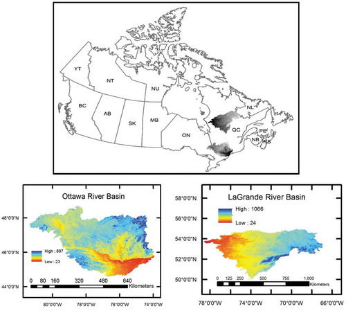
The LGRB drains into La Grande River. It is in north-central Quebec (see Fig. 1), with the total drainage area of nearly 209 000 km². According to the Advanced Very-High-Resolution Radiometer (AVHRR) land cover product for Quebec, 97% of the basin area is covered by forest, with waterbodies composing the other 3%; hence, almost the entire basin is undeveloped. Snow monitoring stations in the LGRB are either snow course sites operated by Hydro-Quebec, or from Environment and Climate Change Canada (ECCC). Stations have monthly visits in winter months (i.e. January–April); however, due to the availability and accessibility, maintaining regular measurements is often limited (Coulibaly and Keum 2016).

The ORB is located on the Ontario-Quebec border northwest of Ottawa. The basin has a drainage area of 146 300 km². The Ottawa River has many tributaries including the Outaouais River, the Montreal River, the Kipawa River, the Madawaska River, the Gatineau River and the Lievre River. Almost 75% of the basin is covered in forest, about 6% of the basin is farmland and less than 2% of the land area has been developed. A digital elevation model of the basin is shown in Fig. 1.

2.2 Data gathering and preparation

2.2.1 Observed snow data

The main source for SWE data was the historical snow course compilation for Canada prepared by the ECCC, supplemented with the Quebec snow course data maintained by the Quebec Ministère du Développement durable, de l’Environnement et des Parcs (MDDEP), which includes observations from Hydro-Quebec, Alcan and the Churchill Falls Power Corporation. Data for stations up to 10 km outside the basins were also included for the interpolation of SWE.

Most of the observations are made at the beginning and the middle of each month, meaning that snow data from the 1st and 15th of January–May in 2010–2016 are considered for the analysis. When more observations are recorded, the snow values for these two days (1st and 15th) in each month are estimated by averaging the daily snow observations over a ± 5-day window.

2.2.2 SNODAS SWE estimates

Snow water equivalent products of SNODAS are downloaded from the National Snow and Ice Data Center (NOHRSC 2004). The temporal resolution of data is one day. For evaluation and comparison with the interpolated/observed SWE, data are averaged considering a ± 5-day window.

2.2.3 Historical hydro-meteorological data for streamflow modelling

For streamflow simulation incorporating the SWE data, two hydrological models, which have been already calibrated for some of the sub-basins in the LGRB (Keum et al. 2018), are used. The models are driven for 2013–2014 with a daily time step considering the availability of historical and SNODAS data. Input data to the models include maximum and minimum temperature, precipitation and SWE. Historical streamflow, temperature and precipitation for the stations in the sub-basins are obtained from Hydro-Quebec. To build up the time-series of SWE data, average values for SNODAS estimates of SWE corresponding to the grids that cover the sub-basins is calculated and used.

2.3 Methods

This section provides details on the proposed methodology for evaluating the potential benefit of SNODAS SWE in hydrological modelling. First, the interpolation technique employed for spatial distribution of snow observations is described. Then, the method used for bias correction of SNODAS SWE based on the interpolated data is explained. Finally, the hydrological models used for streamflow simulation, as well as the criteria used for performance evaluation of the models, are presented.

2.3.1 Interpolation of SWE: geostatistical simulation

To compare gridded SWE products of SNODAS with filled observations, a Gaussian geostatistical simulation technique, called turning band method with external drift, is used (Christakos 1992). This method interpolates in situ measurements of SWE to develop 1-km gridded SWE product. The turning band method is a powerful mathematical operator (Christakos 1992), which reduces two-dimensional simulation to several independent one-dimensional simulations defined on a line equally distributed in two dimensions (Brooker 1985). The idea is to simulate a target variable using an auxiliary linear correlated variable known at the nodes of the result grid file (Bourennane et al. 2000). Geostatistical simulation results in many realizations that, while keeping the sample data characteristics, regenerate the associated statistical and spatial features (Vann et al. 2002). The method represents a reasonable trade-off between quality and computational time effort. This makes the analysis even more efficient for river basins in Canada given that the snow data are sparse in these basins. This geostatistical technique has been successfully used in previous studies for the interpolation of SWE over basins in eastern Canada (Tapsoba et al. 2005, Brown and Tapsoba 2007, Brown et al. 2018) to develop gridded SWE products with a spatial resolution (i.e. 10 km) lower than the resolution targeted in this study. Detailed analysis of the employed interpolation method shows that the impact of the interpolation error on the product evaluation statistics is relatively small (Brown et al. 2018).

To explain the distribution of a variable such as SWE, geostatistics can be defined according to the concept of random function, e.g. $F\left(x\right)$ (Buttafuoco et al. 2012). Then, a set of unknown values is constituted as a set of spatially dependent random variables shown by $F\left(x_{\alpha }\right)$, where $\alpha$ represents sampling points in the range of $1,\dots ,n$. Each observed (measured) value of the variable at location $x_{\alpha }$, is considered as a unique realization of a random variable $F\left(x_{\alpha }\right)$. Variation in the variable $\mathrm{S}\mathrm{W}\mathrm{E}\left(x\right)$, is composed of a deterministic ($m\left(x\right)$) and a stochastic ($ϵ\left(x\right)$) component (Buttafuoco et al. 2010):

(1) $\mathrm{S}\mathrm{W}\mathrm{E}\left(x_{\alpha }\right)=m\left(x\right)+ϵ\left(x\right)$(1)

with $E\left[\mathrm{S}\mathrm{W}\mathrm{E}\left(x\right)\right]=m\left(x\right)$, where E represents expected value. The deterministic component is called the drift, and the stochastic component has a mean value of zero and variogram ${\gamma }_{\epsilon }\left(h\right)$. In the kriging method with an external drift, the deterministic component is usually estimated as a linear regression model of smoothly varying k external variables $y_i\left(x\right),i=1,\dots .,k$:

(2) $m\left(x\right)=a_0\left(x\right)+{\sum }_{i=1}^k{a}_i\left(x\right)y_i\left(x\right)$(2)

where $a_0\left(x\right)$ and$a_i\left(x\right)$are the intercept and coefficients corresponding to the variables of the linear function. The unknown coefficients are considered constant within the search domain and obtained by the kriging method (Goovaerts 1997). Detailed information on the geostatistical simulation algorithm can be found in the previous studies such as Goovaerts (1997) and Chiles and Delfiner (1999), among others.

The SWE cannot be assumed stationary at the regional scale. The idea is to perform SWE simulation using auxiliary linear correlated variables, as explained above, which are known at the nodes of the resultant grid file. The auxiliary correlated variables considered in this study included latitude, longitude, land cover classification generated by the Laurentian Forestry Centre of Natural Resources Canada¹ and surface elevation above sea level obtained from the US Geological Survey (USGS).² The surface elevation is the most important variable describing large-scale snow variability with a good linear correlation with SWE. Surface elevation varies smoothly in space, and this avoids instability of the kriging method with external drift (Goovaerts 1997).

Simulations using geostatistics can be unconditional or conditional. Unconditional simulations regenerate specific statistical characteristics (e.g. mean, variance and covariance function) of a variable without taking into account the filled measurements (observations). In contrast, conditional simulation generates realizations that incorporate the correlation structure of the data and reproduce random components of the variable, which is smoothed out using the kriging method. In the turning band method, considering conditional simulation with external drift, the multi-Gaussian random field model is employed. The following steps are taken in this study as suggested by Chiles and Delfiner (1999):

Step 1. A representative distribution of SWE data is calculated, by weighting each value depending on the geometrical configuration of the associated location. This procedure, called de-clustering, aims at down-weighting the data that are spatially clustered, which contains redundant information (Deutsch and Journel 1992). For a regular sampling design, the data can be associated with the same weights.

Step 2. A linear regression model is executed between SWE data and the auxiliary variables to obtain residuals.

Step 3. The residuals are transformed into normal scores by the use of a Gaussian anamorphosis model which presents features of a non-linear Gaussian function (Rivoirard 1994, Chiles and Delfiner 1999, Wackernagel 2003), while accounting for the previously calculated de-clustering weights.

Step 4. The experimental residual variogram is computed and then fitted with a theoretical model.

Step 5. A Gaussian random field is simulated at the target data locations, conditionally to the available data (i.e. so that the simulations at the data locations match the data values) using the turning band algorithm to produce the ensemble of realizations.

Step 6. The simulations are back-transformed to the original scale (SWE values) to compute mean and standard deviation at each grid. Consequently, maps of the expected values, standard deviations, and quantiles could be generated.

2.3.2 Bias-correction for SNODAS estimates: CDF matching

To use SNODAS estimates of SWE for hydrological modelling, they need to be bias-corrected against snow ground observations. Matching the cumulative distribution functions (cdfs) of data sets based on polynomial fitting is used to remove the systematic differences between the interpolated data and SNODAS SWE. This method has been used for matching the soil moisture data by Brocca et al. (2011), Reichle and Koster (2004), and Kornelsen and Coulibaly (2014). Leach et al. (2018) successfully used a cdf-matching method to correct the SNODAS snow depth estimates based on the snow depth observations from the Environment and Climate Change Canada, for the Don River Basin in Ontario, Canada. Based on this method, the empirical cdf of the observed data is used, and then the cdf of the SNODAS estimates is matched to the cdf of historical data. A third-degree polynomial model is employed for this purpose:

(3) $\mathrm{B}\mathrm{S}=p_1{S}^3+p_2{S}^2+p_{3}S+p_4$(3)

where S is the raw SNODAS SWE data, BS is the bias-corrected SNODAS SWE and $p_1$ to $p_4$ are the coefficients of the polynomial model.

Considering the area of the basins, a large number of gridded data is analysed. To improve the performance of the bias-correction method, the grids are categorized based on their elevation using the k-means clustering method. With the number of clusters to vary between 1 (no clustering, all data to be considered at once) and 4 (classifying data to four groups), four scenarios of data clustering are investigated for bias correction. To identify the most appropriate number of clusters, the silhouette coefficient (Rousseeuw 1987) is calculated. Silhouette coefficient is a measure of the distance between the clusters. The silhouette, ranging between – 1 and 1, indicates how close each point in one cluster is to points in the neighbouring clusters. Silhouette values near +1 show that the sample is far away from the other clusters, 0 indicates that the sample is on or very close to the boundary between two neighbouring clusters and negative values indicate that samples might have been assigned to the wrong cluster. Then, the interpolated data are compared with the SNODAS estimates, before and after bias correction, considering four different clustering scenarios. For this purpose, several evaluation metrics are used to investigate which clustering scenario results in the highest performance (less error between the interpolated and bias-corrected SNODAS SWE). Moreover, for each date, the ground-based observations are compared with the SNODAS estimates of SWE corresponding to the grids closest to the stations.

2.3.3 Streamflow simulation

The McMaster University-Hydrologiska Byråns Vattenbalansavdelning (MAC-HBV) and Sacramento soil moisture accounting (SAC-SMA) models are used for streamflow simulation. The MAC-HBV model, a combined rainfall–runoff and regionalization model based on the original HBV model (Bergström 1976), was originally developed for the estimation of continuous streamflow in gauged and ungauged basins located in the province of Ontario (Samuel et al. 2011, 2012). The SAC-SMA model is a spatially continuous soil moisture accounting model to simulate runoff within a basin (Vrugt et al. 2006). Both MAC-HBV and SAC-SMA are lumped, conceptual rainfall–runoff models. The snow routine that is used in both the models to account for snowmelt is based on the degree-day method.

The MAC-HBV model (with 14 parameters) and the SAC-SMA model (with 18 parameters) have been previously calibrated for some of the sub-basins of the LGRB, for a 2-year period of daily historical data, using observed SWE, temperature and precipitation as input, and the degree-day snow routine method (Keum et al. 2018). To investigate the performance of the bias-corrected SNODAS estimates of SWE for streamflow simulation the models are set up for two sub-basins (one with a low number of ground-based snow stations and the other with a high number). The simulation performance of the models is then measured and compared considering using SWE (i.e. interpolated data, raw SNODAS estimates, bias-corrected SNODAS SWE and observed data) and without SWE. Application of the aforementioned hydrological models for streamflow simulation in the study sub-basins using the bias-corrected SNODAS SWE has not been published/reported yet.

2.3.4 Performance evaluation criteria

The standard metrics of correlation – Nash-Sutcliffe efficiency (NSE), coefficient of determination (R²) – and mean squared error are used to assess the results from matching the cdf of SNODAS SWE against the gridded local SWE values. These criteria are further utilized to measure the simulation performance of the hydrological models:

(4) $\mathrm{N}\mathrm{S}\mathrm{E}=1-\left[\sum _{i=1}^n{(O_i-S_i)}^2/\sum _{i=1}^n{(O_i-{\tilde{O}}_i)}^2]\right]$(4)

(5) $R^2=1-\left[\sum _{i=1}^n{\left|S_i-O_i\right|}^2/\sum _{i=1}^n{\left(\left|S_i-\tilde{O}\right|+\left|O_i-\tilde{O}\right|\right)}^2\right]$(5)

where O_i and S_i are interpolated data and estimated SWE in grid i, respectively. $\tilde{O}$ and $\tilde{S}$ are the mean values of interpolated and estimated SWE, respectively. The NSE represents a measure of the proportion of the initial variance accounted for by the model that ranges from – ∞ to +1 for a perfect correlation. Bias is defined as an average of all errors. The R² compares the difference between the mean of the interpolated data and estimated SNODAS SWE, indicating the degree of error (Gardner and Dorling 2000, Chaloulakou et al. 2003, Sousa et al. 2007). This value varies between 0 for complete disagreement and 1 for perfect agreement between the two sets of data, respectively (Willmott et al. 1985).

The observed SWE at the ground stations is compared with SNODAS estimates of SWE (before and after bias correction) at the nearest grids (within a distance of 400 m). Similarly, interpolated SWE at grids is compared with the corresponding gridded information of SNODAS SWE (before and after bias correction). For the performance evaluation of hydrological modelling, simulated streamflow is compared with the observed streamflow.

3 Results and discussion

It should be noted that the dates to present results in this section are randomly selected (amongst the limited dates with available observations) to show the performance of the developed models over the entire time period (given that the bias-correction method is applied on a daily basis).

3.1 Geostatistical simulation for SWE interpolation

Application of the geostatistical interpolation method for spatial estimation of 1-km gridded SWE values is illustrated for 1 April 2011 for the ORB, as an example, following the steps described in Section 2. The geostatistical analyses were done using the software package ISATIS.³ The same interpolation method has been successfully used in previous studies for the spatial distribution of SWE in Canadian basins (e.g. Tapsoba et al. 2005, Brown and Tapsoba 2007). Most recently, Brown et al. (2018) used this method to estimate 10‐km gridded maximum SWE values in February, March and April, for the Saint‐Maurice Basin in Quebec.

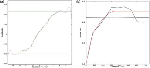
Figure 2(a) and (b) presents histograms of, respectively, the residuals and the normal transformed residuals for 1 April 2011 in the ORB. Figure 3(a) shows the normal transformed residuals, by Gaussian anamorphosis, overlain onto the experimental curve of the residual. The Gaussian variogram of residuals is depicted in Fig. 3(b). This variogram for this date is obtained by combining two model variograms. The choice of a variogram model is based on two spherical nested structures (S1: spherical range = 91.35 km, sill = 0.45; and S2: spherical range = 344.83 km, sill = 0.81).

Figure 2. Histograms of (a) the residuals and (b) the normal transformed residuals from geostatistical simulation for 1 April 2011 in the ORB.

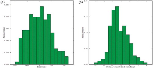
Figure 3. (a) The Gaussian anamorphosis model (line) overlies the experimental curve (dots) of the residuals, and (b) variogram of residuals from geostatistical simulation for 1 April 2011 in the ORB.

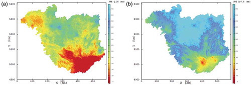
The cross-validation technique (Goovaerts 1997, Chiles and Delfiner 1999) is used to evaluate the consistency between observations and the residual variogram model. The key values of the output are the root mean square error (RMSE; close to zero is ideal) and the variance of the standardized RMSE (close to one is ideal). The goodness of fit evaluated by cross-validation was satisfactory for this date and all other dates (see Table 1 for the ORB for 1 April 2011). The simulations were generated using the conditional turning band method which is a Gaussian simulation technique requiring a multi-Gaussian framework (Matheron 1973). The only parameter of this method is the count of bands, which have been fixed to 600 in this study. The number of realizations was fixed at 100 because a high level of accuracy is reached only when the number of runs is sufficiently large. Figure 4(a) and (b) shows, respectively, the mean and standard deviation of interpolated SWE for 1 April 2011 for the ORB, and Fig. 5(a) and (b) shows the quantiles $Q2.5$ and $Q97.5$, respectively, for the same date.

Table 1. Cross-validation results for the interpolation (geostatistical simulation) of snow observation in ORB, 1 April 2011.

Metric	Mean (cm)	Variance (cm)
Error	1.89	38.71
Standard error	0.02	1.09

Figure 4. (a) Mean SWE estimation map, and (b) SWE standard deviation map of geostatistical simulation over the ORB for 1 April 2011.

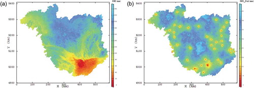
Figure 5. (a) Q2.5 quantile map, and (b) Q97.5 quantile map of geostatistical simulation for SWE over the ORB for 1 April 2011.

3.2 Bias correction of SNODAS SWE

Geostatistical simulation provides interpolated SWE over the basins for grids with a size of 1 km × 1 km. The grids are associated with latitude and longitude. Using the ArcGIS software and digital elevation models (DEMs), elevation data for the grids are extracted. This way, each grid is assigned an elevation. The grids are checked against the network of SNODAS products, where each node is associated with a latitude and a longitude, to identify the SNODAS grid and the corresponding SWE value which is closest to each interpolated cell. Then, for each grid, the snow data, including interpolated SWE and the SNODAS SWE, is categorized into 2–4 clusters based on the corresponding elevation. Table 2 shows the results for k-means clustering (silhouette coefficients) to classify the grids of the basin based on the elevation obtained from the DEMs. As indicated in Table 2, the silhouette values are positive for 2–4 clusters; therefore, bias correction is performed considering binning data to 2, 3 and 4 classes.

Table 2. Clustering results: minimum and maximum elevation in each cluster, and the corresponding silhouette coefficient, for ORB and LGRB based on the grid elevation.

ORB	1 class (no clustering)	2 classes (silhouette: 0.61)		3 classes (silhouette: 0.59)			4 classes (silhouette: 0.55)
		Class 1	Class 2	Class 1	Class 2	Class 3	Class 1	Class 2	Class 3	Class 4
Elevation (m)	Min: 19 Max: 898	Min: 19 Max: 282	Min: 283 Max: 898	Min: 19 Max: 243	Min: 244 Max: 363	Min: 364 Max: 898	Min: 19 Max: 230	Min: 231 Max: 317	Min: 318 Max: 389	Min: 390 Max: 898
LGRB	1 class (no clustering)	2 classes (silhouette: 0.61)		3 classes (silhouette: 0.57)			4 classes (silhouette: 0.53)
		Class 1	Class 2	Class 1	Class 2	Class 3	Class 1	Class 2	Class 3	Class 4
Elevation (m)	Min: 0 Max: 1077	Min: 0 Max: 404	Min: 404 Max: 1077	Min: 0 Max: 300	Min: 300 Max: 493	Min: 493 Max: 1077	Min: 0 Max: 288	Min: 288 Max: 459	Min: 459 Max: 591	Min: 591 Max: 1077

It should be noted that the bias-correction method used matches the cdf of the SNODAS SWE to the cdf of the interpolated data (obtained from the distribution of the observations). Leach et al. (2018) used a similar cdf-matching technique to bias-correct the snow depth products by SNODAS based on the snow observations for the Don River Basin in Ontario (eastern Canada). They showed that raw SNODAS snow products are overestimated, while the corrected SNODAS snow can be utilized to obtain an acceptable estimate of average value for the basin’s SWE.

In the following, for each date, bias correction is performed on SNODAS SWE considering different numbers of the clusters. To investigate how clustering can improve adjusting the SNODAS product to the interpolated SWE, observed ground-based snow data are also used. For this purpose, the nearest SNODAS grid to the location of each observation gauge (within a distance of 400 m) is identified. Then the two datasets – observed SWE from the ground stations and the corresponding identified SNODAS SWE – are compared before and after performing the bias correction on the SNODAS estimates. The performance of the bias-correction method to adjust the SNODAS data is investigated considering the interpolated SWE data for the entire basin by comparing the SWE values of the grids.

The analysis was performed on data for the 1st and 15th day of the month, for January–May 2010–2016. Among the results, for each basin, one date is randomly selected to present the findings. Table 3 compares the observations (ground-based data) against the SNODAS estimates, at the nearest grids, before and after bias correction on 15 March 2016 for the ORB and 1 April 2016 for the LGRB. Table 3 also shows the results of comparing interpolated SWE data with the SNODAS SWE before and after the bias correction.

Table 3. Performance evaluation of the bias-correction method to adjust SNODAS SWE to the interpolated data against a different number of clusters, by comparing the SNODAS grid estimates of SWE with the observed data at stations, as well as the interpolated data for ORB, 15 March 2016, and LRGB, 1 April 2016. NSE: Nash-Sutcliffe efficiency; R²: coefficient of determination.

Before bias correction		After bias correction
Metric		Number of clusters
		1	2	3	4
ORB, 15 March 2016
Observed station data vs SNODAS SWE estimates
NSE	0.14	0.38	0.40	0.64	0.61
R^2	0.78	0.80	0.81	0.89	0.88
Interpolated data vs SNODAS SWE estimates
NSE	0.15	0.40	0.46	0.64	0.66
R^2	0.80	0.83	0.85	0.91	0.91
LRGB, 1 April 2016
Observed station data vs SNODAS SWE estimates
NSE	–0.15	0.69	0.69	0.86	0.91
R^2	0.82	0.93	0.94	0.97	0.98
Interpolated data vs SNODAS SWE estimates
NSE	–0.92	0.19	0.54	0.63	0.67
R^2	0.64	0.77	0.87	0.90	0.91

Analysing the bias-corrected SNODAS SWE and comparing them with the interpolated data, from 2010 to 2016 for the ORB and from 2013 to 2016 for the LGRB, shows that clustering data into 3 or 4 classes results in the highest performance. Based on this analysis, the error in the raw estimates of SNODAS data is decreasing from 2010 to 2016. Considering the results for all dates for two basins, the bias-correction method can improve the agreement of SNODAS estimates of SWE with the observations by up to 70% based on the NSE criterion.

Figure 6 graphically compares the observed SWE data at the six snow gauge stations with the SNODAS estimates of SWE (at the closest grids) before and after bias correction for 1 May 2013. This figure is provided for the LGRB since there are few ground-based stations for this basin, which makes it possible to provide a clear graphical comparison.

Figure 6. Observed SWE at the snow stations against the SNODAS SWE before and after the bias correction for the LGRB, 1 May 2013, and location of the station on the basin map.

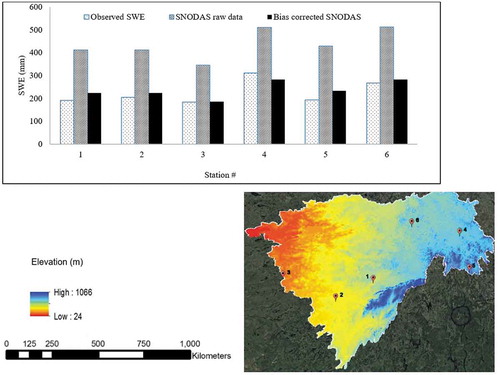
Comparing the observed and interpolated SWE data with the bias-corrected SNODAS SWE confirms that the applied method for adjusting the SNODAS products has been successful.

3.3 Streamflow simulation

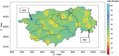
To investigate how incorporating the SWE data in hydrological modelling can affect the streamflow simulation, SNODAS SWE estimates are used in the MAC-HBV and SAC-SMA models for two LGRB sub-basins, Caniapiscau (SB1), where the accuracy of the interpolation is higher due to larger number of ground-based snow stations, and La_Grande_2_et_Lac_Sakami (SB2), where the accuracy of the interpolation is lower. Figure 7 shows these two sub-basins and the distribution of the ground-based snow stations that are used for the interpolation for a specific date, 1 April 2013. For other days, the distribution of the stations is almost the same. These two sub-basins are selected considering the availability of the calibrated hydrological models for the basins, input data and the spatial distribution of the snow gauges on the ground. It should be noted that observed historical data for these sub-basins is available up to 2014 and SNODAS estimates of SWE for this basin are available from 2013 onward. Therefore, a simulation period of 2 years (2013–2014) is used for hydrological modelling.

Figure 7. Location of the two LGRB sub-basins selected to evaluate the performance of hydrological modelling as well as the distribution of the ground-based snow stations used for interpolation for 1 April 2013. SB: sub-basin.

Historical daily data for these sub-basins are pre-processed to be used as input to the models. A one-year period, 1 January 2012 to 31 December 2012, was used to spin up the hydrological models. Since data for more than one meteorological station is available for each sub-basin, the Thiessen polygon method is employed to average the data and build up the time series of inputs. The results of streamflow simulation for the two sub-basins are shown in Fig. 8. It should be noted that the snow data for the sub-basins are only available for the first day of the month, from March to May 2013–2014.

Figure 8. Comparison of streamflow simulation with and without snow data for SB1 with (a) MAC-HBV and (b) SAC-SMA models, and SB2 with (c) MAC-HBV and (d) SAC-SMA models.

Figure 8 highlights the importance of incorporating SWE in hydrological modelling, particularly for high flows and spring runoff simulation. In the case where no SWE is used in the input set, the streamflow peaks are considerably under-estimated by the models. Figure 8 also indicates that the application of SNODAS SWE without correction results in over-estimating the magnitude of peak flows and shifting the time of peak. To the knowledge of the authors, application of bias-corrected SNODAS SWE for streamflow simulation in eastern Canadian basins has not been reported in the previous studies. In a hydrological study for several watersheds in the eastern USA (drainage areas ranging from 5273 to 17 115 km²), where Gyawali and Watkins (2013) used raw SNODAS SWE for calibration of the snowmelt method in HEC-HMS model, comparison of simulated and observed hydrographs indicated that, although low flows are relatively well captured, winter and early spring peak flows are underestimated. In another study by Liu et al. (2015), SNODAS snow depth estimates were used as an independent dataset to evaluate the effect of assimilating bias-corrected snow depth, from the Advanced Microwave Scanning Radiometer for the Earth Observing System (AMSR-E), on streamflow simulation for the Upper Colorado River Basin, USA. Their results suggested that application of raw SNODAS snow products will result in overestimation of streamflow, especially at high elevations.

In addition to the SWE products of SNODAS (both raw and bias-corrected), gridded interpolated SWE, as well as the observed SWE for the stations within the sub-basins, are also used to drive the hydrological models. To build up the time-series of snow data based on the station observations (the number of which varies between 2 and 5 depending on the date), the Thiessen polygon method is used to obtain an average value of SWE for the sub-basins. Based on the results, the simulation performance of the models when observed station data are used as input is almost the same as when an average of the interpolated data is used to build up the time-series of SWE data. This further confirms that the applied interpolation method has been successful in estimating the gridded snow data. To further assess the performance of the streamflow modelling, Table 4 is provided.

Table 4. Streamflow simulation performance for SB1 and SB2 in LGRB without SWE, with raw and bias-corrected SNODAS SWE as well as with interpolated SWE (2013–2014).

Metric	Model
	MAC-HBV				SAC-SMA
	No SWE	Raw SNODAS SWE	Bias-corrected SNODAS SWE	Interpolated SWE	No SWE	Raw SNODAS SWE	Bias-corrected SNODAS SWE	Interpolated SWE
SB1
NSE	0.86	–0.69	0.89	0.79	0.63	0.11	0.85	0.83
R^2	0.95	0.78	0.97	0.95	0.86	0.84	0.95	0.95
SB2
NSE	–0.74	–0.99	0.27	0.28	0.39	–0.39	0.75	0.72
R^2	0.49	0.73	0.83	0.84	–0.44	0.32	–0.13	–0.06

Table 4 shows that application of the bias-corrected SNODAS SWE improves the hydrological simulation performance for the sub-basins. For the first sub-basin (SB1 in Table 4), the metrics have their worst values when raw SNODAS SWE without any processing is used. Table 4 also shows that the performance of hydrological modelling when bias-corrected SNODAS SWE is used is as good as, and in most cases even better than, when the interpolated snow data are used.

The observed snow data were only available for the first day of the month from March to May; therefore, the interpolated data could be used for bias correction of the SNODAS SWE for the same dates. However, since daily values of SNODAS products are available, it is decided to investigate if the application of daily snow data could improve the performance of hydrological modelling. For this purpose, the adjustment equation which is obtained for bias-correcting data for the first day of a month is used to correct the SNODAS SWE data for the remaining days in that month. Preliminary results show that application of daily bias-corrected SNODAS SWE for May would significantly overestimate the simulated streamflow. Therefore, only daily snow data are used for the other two months. The intention here is to investigate if the application of bias-corrected SNODAS estimates can outperform the results of hydrological modelling, in comparison with the application of interpolated snow, particularly for SB2 where the number of ground stations is low, and the accuracy of the interpolation is not high. Tables 5 and 6 show the results of this comparison. It should be noted that where one value of SWE in a month is used in the input sets of the models, to build up the daily time-series of SWE, values of SWE for the other days are estimated by the snowmelt component of the hydrological model (i.e. degree-day method).

Table 5. Comparison of the performance of hydrological models for the simulation of daily streamflow for SB1 and SB2 when either interpolated SWE (one value in a month) or bias-corrected SNODAS SWE (one value a month as well as daily values) is used in hydrological modelling.

Metric	MAC-HBV				SAC-SMA
	SB1		SB2		SB1		SB2
Interpolated SWE
NSE	0.79		0.29		0.83		0.72
R^2	0.96		0.84		0.96		0.94
	One SWE in month	Daily SWE	One SWE in month	Daily SWE	One SWE in month	Daily SWE	One SWE in month	Daily SWE
Bias-corrected SNODAS SWE
NSE	0.89	0.9	0.28	0.37	0.86	0.87	0.75	0.8
R^2	0.96	0.98	0.83	0.86	0.96	0.96	0.94	0.96

Table 6. Comparison of the performance of hydrological models for the simulation of streamflow peak values for SB1 and SB2 when either interpolated SWE (one value a month) or bias-corrected SNODAS SWE (one value a month as well as daily values) is used in hydrological modelling.

Metric	MAC-HBV				SAC-SMA
	SB1		SB2		SB1		SB2
Interpolated SWE
NSE	0.94		0.45		0.82		0.68
R^2	0.99		0.84		0.94		0.92
	One SWE in month	Daily SWE	One SWE in month	Daily SWE	One SWE in month	Daily SWE	One SWE in month	Daily SWE
Bias-corrected SNODAS SWE
NSE	0.95	0.95	0.43	0.45	0.78	0.82	0.65	0.61
R^2	0.99	0.99	0.83	0.84	0.93	0.95	0.90	0.91

Table 5 shows that application of daily values of bias-corrected SNODAS SWE estimates results in slightly improving the simulation performance of hydrological models, particularly for SB2. Considering the significant role of SWE in the formation of spring runoff and flood events, an analysis is performed on peak values of streamflow. For this purpose, the peak over threshold method is employed to identify the peaks in the time-series of observed streamflow. Then, they are compared with the corresponding values of streamflow simulated considering the incorporation of interpolated SWE as well as the bias-corrected SNODAS SWE in the hydrological models. The results are presented in Table 6.

Table 6 indicates that both models perform well in the simulation of spring peak flow particularly for SB1. Based on the results, the application of daily SWE data slightly improves the simulation of peak flow values. However, using only one value of SWE for streamflow simulation still shows high performance. This could be attributed to the fact that the hydrological models are calibrated based on the available observed SWE data (where there is only one data available a month). The performance of peak flow simulation when bias-corrected SNODAS SWE is used in the hydrological modelling is as good as when the interpolated SWE is utilized.

4 Summary and conclusions

The SWE plays an important role in the simulation and forecasting of spring runoff and probable floods from snowmelt. However, due to the hardship in measuring snow data in cold weathers and high elevations, application of the snow estimates provided by the assimilated systems in hydrological modelling has gained interest. SNODAS is an assimilation system that integrates model analysis with filled measurements and other sources of data to provide estimates of daily snow products at a 1-km² resolution for the USA and the southern part of Canada. We evaluated the accuracy of the SNODAS SWE products for streamflow simulation in two large basins (with areas of more than 140 000 km²) across eastern Canada. The validation of SNODAS products for the selected basins is independent of the ground-based observations integrated into the SNODAS production process. Therefore, SNODAS products are compared directly with credible point-based ground observations.

Given that SNODAS data are provided for grids of 1-km² resolution, a geospatial interpolation method is employed for distribution of snow observations, obtained from the ground-based stations, over the basins to provide gridded SWE data to be compared with SNODAS products. Then, the SNODAS estimates are adjusted through reducing bias based on the CDF of the interpolated data and cluster analysis on elevation. Following the bias-correction, application of the bias-corrected SNODAS estimates in hydrological modelling is investigated.

Comparing the SNODAS SWE before and after bias reduction with the interpolated and observed SWE indicates that bias-correcting SNODAS estimates of SWE significantly improves the accuracy of these products. The results show that incorporating SNODAS SWE estimates without bias correction for hydrological modelling in eastern Canadian basins results in the overestimation of streamflow and peak flow values.

Although the employed hydrological models are not distributed, their simulation performance following the incorporation of the bias-corrected SNODAS SWE is reasonably high and acceptable. For the current study, these models are considered sufficient since in the selected sub-basins, runoff is not mainly generated only by snowmelt (the average snowmelt contribution to the peak flow values is 30%). Moreover, the hydrological simulation results show that the degree-day method, used by the models to convert the distributed bias-corrected SWE to snowmelt, works well enough. Therefore, distributed snow information has been operationally used to estimate snowmelt in lumped rainfall-runoff models. The hydrological models in this study were calibrated using limited SWE observations (two values a month). Given that SNODAS products are provided in high temporal resolution (i.e. daily), re-calibration of the hydrological models using daily bias-corrected SNODAS SWE is suggested. Moreover, for watersheds with a significant difference in topographic expression, developing distributed hydrological models (such as WATFLOOD which is now an open source software and a relatively easy distributed model to set up) and calibration with spatially distributed bias-corrected SNODAS products is expected to improve the performance of streamflow simulation. Absence of data was also a limitation to the bias-correction method. In this study, bias correction of SWE was performed on a daily basis. However, developing a correction equation that could work throughout the year, or for example seasonal correction equations could be more efficient. As per the geostatistical simulation method, like other probabilistic approaches, it is necessary to have data of quality and in large numbers. In this method, the variogram modelling is an important step and having enough information is necessary to accurately estimate it.

Investigating the performance of hydrological models incorporating the raw and bias-corrected SNODAS SWE indicates that although these products are biased for eastern Canadian basins, bias correction could result in relatively high performance for spring runoff simulation, particularly for sub-basins which contain few stations with available snow observations. Good estimation of SWE is of great importance for short/long term spring runoff forecasting to support water management, flood forecasting, and reservoir operations.

Acknowledgements

The authors are grateful to the Marc Durocher and Samer Alghabra from Hydro-Québec for providing some data, the National Operational Hydrological Remote Sensing Center for providing SNODAS products, and for data available from Environment and Climate Change Canada.

Disclosure statement

No potential conflict of interest was reported by the authors.

Additional information

Funding

This research was supported by the Natural Science and Engineering Research Council (NSERC) of Canada [grant NSERC Canadian FloodNet – NETGP-451456].

Notes

¹ http://www.nrcan.gc.ca/forests/measur-ing‐reporting/remote‐sensing/13433.

² https://nationalmap.gov/small_scale/atlasftp.html.

³ https://www.geovariances.com.

References

- Aagaard, K. and Carmack, E.C., 1989. The role of sea ice and other fresh water in the Arctic circulation. Journal of Geophysical Research, 94, 14485. doi:10.1029/JC094iC10p14485
- Anctil, F., et al., 2004. A soil moisture index as an auxiliary ANN input for stream flow forecasting. Journal of Hydrology, 286, 155–167. doi:10.1016/j.jhydrol.2003.09.006
- Anderson, B.T., 2011. Spatial distribution and evolution of a seasonal snowpack in complex terrain: an evaluation of the SNODAS modeling product. MSc thesis. Boise, ID: Boise State University.
- Andrews, J., 1993. Flooding: Canada water book. Ottawa, ON: Environment Canada.
- Armstrong, R.L. and Brodzik, M.J., 2001. Recent northern hemisphere snow extent: a comparison of data derived from visible and microwave satellite sensors. Geophysical Research Letters, 28, 3673–3676. doi:10.1029/2000GL012556
- Bair, E.H., et al., 2015. Comparison and error analysis of reconstructed SWE to Airborne Snow Observatory measurements in the Upper Tuolumne Basin, CA. In: Proceedings of Western Snow conference, Grass Valley, CA.
- Barlage, M., et al., 2010. Noah land surface model modifications to improve snowpack prediction in the Colorado Rocky Mountains. Journal of Geophysical Research, 115, D22101. doi:10.1029/2009JD013470
- Barnett, T.P., Adam, J.C., and Lettenmaier, D.P., 2005. Potential impacts of a warming climate on water availability in snow-dominated regions. Nature, 438, 303–309. doi:10.1038/nature04141
- Beard, L.R., 1992. Hydrology of floods in Canada — A guide to planning and design. Journal of Hydrology, 131, 387–388. doi:10.1016/0022-1694(92)90227-M
- Berg, A.A. and Mulroy, K.A., 2006. Streamflow predictability in the Saskatchewan/Nelson River basin given macroscale estimates of the initial soil moisture status. Hydrological Sciences Journal, 51, 642–654. doi:10.1623/hysj.51.4.642
- Bergström, S., 1976. Development and Application of a conceptual runoff model fro Scandinavian catchment. Sweden: Department of Water Resources Engineering, Lund Institute of Technology, University of Lund.
- Bourennane, H., King, D., and Couturier, A., 2000. Comparison of kriging with external drift and simple linear regression for predicting soil horizon thickness with different sample densities. Geoderma, 97, 255–271. doi:10.1016/S0016-7061(00)00042-2
- BP, 2015. Statistical review of world energy 2015 [online]. Available from: http://www.bp.com/en/global/corporate/energy-economics/statistical-review-of-world-energy.html [Accessed 2 March 2016].
- Brocca, L., et al., 2011. Soil moisture estimation through ASCAT and AMSR-E sensors: an intercomparison and validation study across Europe. Remote Sensing of Environment, 115, 3390–3408. doi:10.1016/j.rse.2011.08.003
- Brooker, P.I., 1985. Two-dimensional simulation by turning bands. Journal of the International Association for Mathematical Geology, 17, 81–90. doi:10.1007/BF01030369
- Brown, R. and Tapsoba, D., 2007. Improved mapping of snow water equivalent over Quebec. In: 64th Eastern Snow conference, St. John’s, Newfoundland, Canada. doi:10.1094/PDIS-91-4-0467B
- Brown, R., Tapsoba, D., and Derksen, C., 2018. Evaluation of snow water equivalent datasets over the Saint-Maurice river basin region of southern Québec. Hydrological Processes, 32, 2748–2764. doi:10.1002/hyp.13221
- Brown, R.D., 2000. Northern hemisphere snow cover variability and change, 1915–97. Journal of Climate, 13, 2339–2355. doi:10.1175/1520-0442(2000)013<2339:NHSCVA>2.0.CO;2
- Buttafuoco, G., Caloiero, T., and Coscarelli, R., 2010. Spatial uncertainty assessment in modelling reference evapotranspiration at regional scale. Hydrology and Earth System Sciences, 14, 2319–2327. doi:10.5194/hess-14-2319-2010
- Buttafuoco, G., et al., 2012. Assessing spatial uncertainty in mapping soil erodibility factor using geostatistical stochastic simulation. Environmental Earth Sciences, 66, 1111–1125. doi:10.1007/s12665-011-1317-0
- Carroll, T.R., et al., 2006. NOAA’s national snow analyses. In: 74th Annual Meeting of the Western Snow conference, Las Cruces, NM, 31–43.
- Chaloulakou, A., Saisana, M., and Spyrellis, N., 2003. Comparative assessment of neural networks and regression models for forecasting summertime ozone in Athens. Science of the Total Environment, 313, 1–13. doi:10.1016/S0048-9697(03)00335-8
- Chiles, J. and Delfiner, P., 1999. Geostatistics: modeling spatial uncertainty Chiles, J. and Delfiner, P. New York: Wiley, 695.
- Christakos, G., 1992. Random field models in earth sciences. Elsevier. doi:10.1016/C2009-0-22238-0
- Clow, D.W., et al., 2012. Evaluation of SNODAS snow depth and snow water equivalent estimates for the Colorado Rocky Mountains, USA. Hydrological Processes, 26, 2583–2591. doi:10.1002/hyp.9385
- Coulibaly, P. and Keum, J., 2016. Snow network design and evaluation for La Grande River Basin. Hamilton, ON: Hydro-Quebec.
- Deutsch, C.V. and Journel, A.G., 1992. Geostatistical software library and user’s guide (GSLIB). New York: Oxford University Press.
- Dozier, J., Bair, E.H., and Davis, R.E., 2016. Estimating the spatial distribution of snow water equivalent in the world’s mountains. Wiley Interdisciplinary Reviews: Water, 3, 461–474. doi:10.1002/wat2.1140
- Dressler, K.A., Fassnacht, S.R., and Bales, R.C., 2006. A comparison of snow telemetry and snow course measurements in the Colorado River Basin. Journal of Hydrometeorology, 7, 705–712. doi:10.1175/JHM506.1
- Erxleben, J., Elder, K., and Davis, R., 2002. Comparison of spatial interpolation methods for estimating snow distribution in the Colorado Rocky Mountains. Hydrological Processes, 16, 3627–3649. doi:10.1002/hyp.1239
- Fassnacht, S.R., Dressler, K.A., and Bales, R.C., 2003. Snow water equivalent interpolation for the Colorado River Basin from snow telemetry (SNOTEL) data. Water Resources Research, 39, 1–10. doi:10.1029/2002WR001512
- Fierz, C., et al., 2009. The international classification for seasonal snow on the ground. IHP-VII Tech. Doc. Hydrology, 83, 90.
- Gardner, M.W. and Dorling, S.R., 2000. Statistical surface ozone models: an improved methodology to account for non-linear behaviour. Atmospheric Environment, 34, 21–34. doi:10.1016/S1352-2310(99)00359-3
- Gingras, D., Adamowski, K., and Pilon, P.J., 1994. Regional flood equations for the provinces of Ontario and Quebec. Journal of the American Water Resources Association, 30, 55–67. doi:10.1111/j.1752-1688.1994.tb03273.x
- Goovaerts, P., 1997. Geostatistics for natural resources evaluation. New York, NY: Oxford University Press Inc.
- Guan, B., et al., 2013. Snow water equivalent in the Sierra Nevada: Blending snow sensor observations with snowmelt model simulations. Water Resources Research, 49, 5029–5046. doi:10.1002/wrcr.20387
- Gyawali, R. and Watkins, D.W., 2013. Continuous hydrologic modeling of snow-affected watersheds in the Great Lakes Basin using HEC-HMS. Journal of Hydrologic Engineering, 18, 29–39. doi:10.1061/(ASCE)HE.1943-5584.0000591
- Harshburger, B.J., et al., 2010. Spatial interpolation of snow water equivalency using surface observations and remotely sensed images of snow-covered area. Hydrological Processes, 24, n/a–n/a. doi:10.1002/hyp.7590
- Hedrick, A., et al., 2015. Independent evaluation of the SNODAS snow depth product using regional-scale lidar-derived measurements. Cryosphere, 9, 13–23. doi:10.5194/tc-9-13-2015
- Hydro-Québec, 2015. Sustainability report: setting new sights with our clean energy, Report 14. Hamilton, ON: Hydro-Québec, 75.
- Irvine, K.N. and Drake, J.J., 1987. Spatial analysis of snow-and rain-generated highflows in Southern Ontario. The Canadian Geographer / Le Géographe Canadien, 31, 140–149. doi:10.1111/j.1541-0064.1987.tb01634.x
- Javelle, P., Ouarda, T.B.M.J., and Bobée, B., 2003. Spring flood analysis using the flood-duration-frequency approach: application to the provinces of Quebec and Ontario, Canada. Hydrological Processes, 17, 3717–3736. doi:10.1002/hyp.1349
- Keum, J., et al., 2018. Application of SNODAS and hydrologic models to enhance entropy-based snow monitoring network design. Journal of Hydrology, 561, 688–701. doi:10.1016/j.jhydrol.2018.04.037
- Kolstad, E.W., 2017. Causal pathways for temperature predictability from snow depth. Journal of Climate, 30, 9651–9663. doi:10.1175/JCLI-D-17-0280.1
- Kornelsen, K.C. and Coulibaly, P., 2014. Data-based disaggregation of SMOS soil moisture. In: 2014 IEEE geoscience and remote sensing symposium, IEEE, 3334–3337. doi:10.1109/IGARSS.2014.6947194
- Leach, J.M., Kornelsen, K.C., and Coulibaly, P., 2018. Assimilation of near-real time data products into models of an urban basin. Journal of Hydrology, 563, 51–64. doi:10.1016/j.jhydrol.2018.05.064
- Liu, Y., et al., 2015. Blending satellite-based snow depth products with in situ observations for streamflow predictions in the Upper Colorado River Basin. Water Resources Research, 51, 1182–1202. doi:10.1002/2014WR016606
- Marsh, P. and Woo, M.-K., 1984. Wetting front advance and freezing of meltwater within a snow cover: 1. Observations in the Canadian Arctic. Water Resources Research, 20, 1853–1864. doi:10.1029/WR020i012p01853
- Matheron, G., 1973. The intrinsic random functions and their applications. Advances in Applied Probability, 5 (3), 439. doi:10.2307/1425829
- Metsämäki, S., et al., 2002. Improved linear interpolation method for the estimation of snow-covered area from optical data. Remote Sensing of Environment, 82, 64–78. doi:10.1016/S0034-4257(02)00025-1
- Moreno, J.I.L., Latron, J., and Lehmann, A., 2009. Effects of sample and grid size on the accuracy and stability of regression-based snow interpolation methods. Hydrological Processess, 24, n/a–n/a. doi:10.1002/hyp.7564
- NOAA, 2018. Sea ice and snow cover extent | snow and ice | National Centers for Environmental Information (NCEI) [online]. https://www.ncdc.noaa.gov/snow-and-ice/extent/snow-cover/nhland/1 [Accessed 2 January 2018].
- NOHRSC (National Operations Hydrologic Remote Sensing Center), 2004. Snow data assimilation system (SNODAS) data products at NSIDC, Version 1 [January 2010–December 2016]. Boulder, CO: National Snow and Ice Data Center (NSIDC). doi:10.7265/N5TB14TC
- Reichle, R.H. and Koster, R.D., 2004. Bias reduction in short records of satellite soil moisture. Geophysical Research Letters, 31, L19501. doi:10.1029/2004GL020938
- Rivoirard, J., 1994. Introduction to disjunctive kriging and non linear geostatistics. New York, NY: Oxford University Press.
- Robinson, D.A., Dewey, K.F., and Heim, R.R., 1993. Global snow cover monitoring: an update. Bulletin of the American Meteorological Society, 74, 1689–1696. doi:10.1175/1520-0477(1993)074<1689:GSCMAU>2.0.CO;2
- Rousseeuw, P.J., 1987. Silhouettes: a graphical aid to the interpretation and validation of cluster analysis. Journal of Computational and Applied Mathematics, 20, 53–65. doi:10.1016/0377-0427(87)90125-7
- Samuel, J., Coulibaly, P., and Metcalfe, R.A., 2011. Estimation of continuous streamflow in Ontario Ungauged Basins: comparison of regionalization methods. Journal of Hydrologic Engineering, 16, 447–459. doi:10.1061/(ASCE)HE.1943-5584.0000338
- Samuel, J., Coulibaly, P., and Metcalfe, R.A., 2012. Identification of rainfall–runoff model for improved baseflow estimation in ungauged basins. Hydrological Processess, 26, 356–366. doi:10.1002/hyp.8133
- Shrubsole, D., et al., 2003. An assessment of flood risk management in Canada. ICLR Research Paper Series no. 28. Toronto, ON: Institute for Catastrophic Loss Reduction.
- Sospedra-Alfonso, R., Merryfield, W.J., and Kharin, V.V., 2016. Representation of snow in the Canadian seasonal to interannual prediction system. Part II: potential predictability and hindcast skill. Journal of Hydrometeorology, 17, 2511–2535. doi:10.1175/JHM-D-16-0027.1
- Sousa, S., et al., 2007. Multiple linear regression and artificial neural networks based on principal components to predict ozone concentrations. Environmental Modeling and Software, 22, 97–103. doi:10.1016/j.envsoft.2005.12.002
- Tapsoba, D., et al., 2005. Apport de la technique du krigeage avec dérive externe pour une cartographie raisonnée de l’équivalent en eau de la neige : application aux bassins de la rivière Gatineau. Canadian Journal of Civil Engineering, 32, 289–297. doi:10.1139/l04-110
- Van Steenbergen, N. and Willems, P., 2013. Increasing river flood preparedness by real-time warning based on wetness state conditions. Journal of Hydrology, 489, 227–237. doi:10.1016/j.jhydrol.2013.03.015
- Vann, J., Bertoli, O., and Jackson, S., 2002. An overview of geostatistical simulation for quantifying risk. In: Proceedings of geostatistical association of Australasia symposium “Quantifying Risk and Error” (2002), Perth, Western Australia, 1–12.
- Vrugt, J.A., et al., 2006. Application of stochastic parameter optimization to the Sacramento Soil Moisture Accounting model. Journal of Hydrology, 325, 288–307. doi:10.1016/j.jhydrol.2005.10.041
- Wackernagel, H., 2003. Multivariate Geostatistics. 3rd ed. Berlin, Germany: Springer, 403.
- Willmott, C.J., et al., 1985. Statistics for the evaluation and comparison of models. Journal of Geophysical Research, 90, 8995. doi:10.1029/JC090iC05p08995
- Wrzesien, M.L., et al., 2017. Comparison of methods to estimate snow water equivalent at the mountain range scale: a case study of the California Sierra Nevada. Journal of Hydrometeorology, 18, 1101–1119. doi:10.1175/JHM-D-16-0246.1
- Zhang, Y.F. and Yang, Z.L., 2016. Estimating uncertainties in the newly developed multi-source land snow data assimilation system. Journal of Geophysical Research Atmospheres, 121, 8254–8268. doi:10.1002/2015JD024248