Evaporation process modelling over northern Iran: application of an integrative data-intelligence model with the krill herd optimization algorithm

ABSTRACT

An integrated data-intelligence model based on multilayer perceptron (MLP) and krill herd optimization – the MLP-KH model – is presented for the estimation of daily pan evaporation. Daily climatological information collected from two meteorological stations in the northern region of Iran is used to compare the potential of the proposed model against classical MLP and support vector machine models. The integrated and the classical models were assessed based on different error and goodness-of-fit metrics. The quantitative results evidenced the capacity of the proposed MLP-KH model to estimate daily pan evaporation compared to the classical ones. For both weather stations, the lowest root mean square error (RMSE) of 0.725 and 0.855 mm/d, respectively, was obtained from the integrated model, while the RMSE for MLP was 1.088 and 1.197, and for SVM it was 1.096 and 1.290, respectively.

KEYWORDS:

• krill herd optimization
• integrated model
• class A pan
• Guilan Province
• Iran

Editor S. Archfield Associate editor N. Malamos

1 Introduction

A large proportion of total renewable water becomes unrecoverable through evaporation from water bodies and soil surface, as well as through transpiration from plant canopies. To properly describe the water balance of basins, lakes, artificial reservoirs, and other water bodies, and also to optimize the use of irrigation water resources, accurate and reliable estimates of evaporation and evapotranspiration rates are always needed, especially in arid or semi-arid regions, where water scarcity often pose a threat to the environment, agriculture, the livelihood security of farmers, and the food security of all people. Estimating the amount of water lost into the atmosphere through the processes of evaporation and evapotranspiration is a complicated task, due to complex interactions exist among evaporation rate, land and plant factors, and climatological variables. Evaporation is typically considered as the most difficult component of the hydrological cycle to estimate (Singh and Xu 1997). In the literature, there are lots of methods proposed to estimate evaporation or evapotranspiration, which can be usually classified into water budget, empirical, mass transfer, energy budget, and combination approaches (Xu and Singh 2000, Gallego-Elvira et al. 2012). In addition to these methods, pan evaporation and lysimeter data, remotely sensed satellite products, large aperture scintillometer (LAS) measurements, and eddy covariance data provided by flux tower networks such as AmeriFlux (Boden et al. 2013), CarboEurope (Valentini et al. 2000), and AsiaFlux (Mizoguchi et al. 2009) can also be used to estimate evaporation or evapotranspiration. Despite numerous studies on evaluating and comparing evaporation estimation methods, there is not yet a general agreement on the superiority of any specific approach or method to the others and the use of a particular method depends on factors such as data availability and quality and objectives of the application.

The Guilan Plain, northern Iran, is known as the second most important rice production area in Iran. Almost all irrigation water in the region is drawn from the Sefidroud River, a large river which rises in the mountains of western Iran and flows for 670.0 km to its mouth on the Caspian Sea. The Guilan Plain is located in the lower course of the river, so the amount of water available in the region mainly depends on the water taken by upstream users. In recent years, the demand for water in the upper parts of the Sefidroud River Basin has increased dramatically and as a result, the Guilan Plain is faced with a serious problem of water scarcity. Evidence has it that the phenomenon of climate change could also increase the rice water requirement in the region (Hadinia et al. 2017), which would, in turn, worsen the problem. Designing and utilizing small artificial ponds to store precipitation received in autumn and spring (out of growing season), implementing new irrigation schedules and methods to improve water use efficiency, and planting crops with low water consumption are recognized as effective ways to tackle the problems that the farmers in the region are facing now. An important step towards solving the water scarcity problem is acquiring accurate and reliable evaporation or evapotranspiration data. Class A pan evaporation is monitored in quite a lot of weather stations throughout Iran. Data collected from this simple and low-cost instrument can be used to estimate evapotranspiration, and evaporation from water bodies (Stanhill 2002, Lim et al. 2016). However, observed pan data could be incomplete, missing, or inaccurate. So, it would be quite useful to have models for estimating pan evaporation from reliable climatological measurements. Such models could also be used to evaluate the outputs of General Circulation Models (GCMs) and to project the effect of climate change on the rate of evaporation or evapotranspiration (Stanhill 2002, Rotstayn et al. 2006).

Generally, there are three approaches to the simulation of a complex physical phenomenon such as pan evaporation: (i) physically-based, (ii) Conceptual, and (iii) Data-based. While physically-based models derived from established physical principles, conceptual models are based on simplified conceptualizations of a physical system (Carcano et al. 2008). Conceptual models for pan evaporation were developed in some studies (e.g. the PenPan model by Rotstayn et al. 2006; the multilayer model developed by Molina Martínez et al. 2006; PenPan-V2C and PenPan-V2S by, Lim et al. 2016). The physical behavior of the complex process of pan evaporation were also investigated in a number of studies (e.g. Chu et al. 2010, Lim et al. 2012). In the case of evaporation or evapotranspiration estimation, data-based or black box models are decent replacements to conceptual models. Numerous studies have been made to develop regression equations to estimate pan evaporation from climatological data such as temperature, vapor pressure, day length, and solar radiation. Early studies by Fitzpatrick (1963) and Clemence (1987), and more recent studies by Almedeij (2012) and Xiong et al. (2012) are examples of regression equations for pan evaporation estimation. Since the early nineties, more sophisticated data-based techniques, such as Artificial Neural Networks (ANNs), fuzzy and neuro-fuzzy systems, Support Vector Machines (SVMs), and relevant vector machines, have been successfully used in a wide spectrum of problems related to water resources management, including, but not limited to, precipitation forecasting, rainfall-runoff modelling, groundwater modelling, water quality assessment, sediment load prediction, and evaporation modelling. An overview of sophisticated data-based techniques and their applications in hydrological fields of study can be found in the papers by Maier and Dandy (2000), Wu et al. (2014), Raghavendra and Deka (2014), Yaseen et al. (2015), and Afan et al. (2016). In the context of estimating or forecasting hydrological random variables, the quantity of measured calibration data, as well as the data quality, is also a significant and influencing factor in choosing neural network-based models as simulation tools. Numerous studies have assessed the abilities of ANNs in pan evaporation modelling (e.g. Ashrafzadeh 1999, Bruton et al. 2000, Sudheer et al. 2002, Keskin and Terzi 2006, Kişi 2006, Tan et al. 2007, Kim and Kim 2008, Rahimikhoob 2009, Piri et al. 2009, Kişi 2009, Keskin et al. 2009, Dogan et al. 2010, Tabari et al. 2010, Nourani and Sayyah Fard 2012, Abghari et al. 2012, Goyal et al. 2014, Malik and Kumar 2015, Wang et al. 2017, Malik et al. 2017). However, finding an optimal parameter set for an ANN model is a challenging issue, and there is no definitive evidence for the superiority of an optimization technique. It is an inevitable fact that ANNs have a non-parsimonious nature, and each neural network-based model uses a large number of parameters to simulate a complex process. Based on this fact, strategies such as selecting the most important influencing factors to reduce the number of input independent variables, and subsequently, the number of parameters to be optimized are usually considered in designing effective neural network-based models. Despite the non-parsimonious nature of ANNs, the level of complexity and nonlinearity of the process to be simulated can usually justify choosing an ANN model that requires so many parameters rather than a conventional highly parsimonious model. However, an appropriate and effective optimization algorithm should be considered to calibrate neural network-based models. Optimization methods that are commonly used to calibrate ANNs and find the optimal values of their parameters are based on the gradient of a predefined loss function, and as a result, these methods may suffer from the problem of local optima. To overcome this problem, bio-inspired optimization algorithms, which use nature-inspired search procedures rather than derivatives to find optimal solutions, are suggested in some studies to train ANNs. Since there are many natural sources of inspiration, a host of nature-inspired optimization algorithms can be found in the literature, but just a few of these algorithms have been used in hydrological studies. Ghorbani et al. (2017a); Ghorbani et al. (2017b), Yaseen et al. (2017), Ashrafzadeh et al. (2018), and Deo et al. (2018) showed that combining neural network-based models with the firefly algorithm, an optimization procedure inspired by the movement of fireflies, results in more accurate estimates of variables such as field capacity, permanent wilting point, streamflow, pan evaporation, and wind speed. In the mentioned studies, the firefly algorithm was integrated with different types of neural networks (multilayer perceptron, adaptive neuro-fuzzy inference system, and support vector machines) to develop integrated models. It was collectively concluded that the firefly algorithm could be used as an effective technique to adjust the parameters of an ANN model. Despite the usefulness of nature-inspired algorithms, one shortcoming of these methods could be that each algorithm uses a set of coefficients whose optimal values need to be determined using a meta-optimization technique (in the case of firefly algorithm, there are at least three adjustable coefficients).

Inspired by the studies focusing on the biological mechanisms of formation of krill swarms, Gandomi and Alavi (2012) proposed the krill herd (KH) optimization algorithm. The KH algorithm is based on minimizing the distance between food location and krill position, and, compared to the other nature-inspired algorithms, has the minimum number of coefficients needed to be fine-tuned (i.e. just one coefficient). The krill herd algorithm mathematically simulate three types of movement of an individual krill, movement due to foraging activities, movement forced by other individuals, and random movements. The first two processes are, respectively, local and global strategies, making KH a powerful optimization algorithm to address the problem of local optima (Mandal et al. 2014). This is a distinct characteristic of the krill herd algorithm, and theoretically makes it superior to other nature-inspired optimization techniques. Kowalski and Łukasik (2016) examined the krill herd algorithm when used to train neural networks and compared its performance with that of conventional and other nature-inspired optimization algorithms. They concluded that KH offers promising performance in terms of error measures and the time consumed in training. Diverse engineering applications of the KH algorithm, such as optimization the operation of power plants (Mandal et al. 2014), data clustering (Jensi and Jiji 2016), simulation of separation processes in chemical engineering (Moodley et al. 2015), designing of small-scale electricity generator networks (Sultana and Roy 2016, Mukherjee et al. 2016), optimal designing of radiative enclosures (Sun et al. 2016), and financial time series forecasting using support vector machines (Stasinakis et al. 2016) has been reported in recent years. However, to the best of our knowledge, the KH algorithm has not been used in the field of modelling hydrological processes. Considering the successful applications of neural network-based models and the KH optimization algorithm in previous studies, we decided to integrate ANN models with KH in order to develop an effective integrated model for simulating the complex process of evaporation. First, using the data gathered in two weather stations in the Guilan Plain, northern Iran, conventional ANNs and SVMs for pan evaporation estimation were developed. Then, the krill herd optimization algorithm was utilized to develop integrated ANN-KH models. The models developed in this study can be used to acquire adequate evaporation datasets for subsequent studies in the study area.

2 Materials and methods

2.1 Classical multilayer perceptron (MLP)

The perceptron, the very basic form of an artificial neural network, is actually a binary classifier and can be described using the following equation:

(1) $f\left(z\right)=\left\{\begin{array}{c}1\mathrm{i}\mathrm{f}z={\mathit{w}}^T\cdot \mathit{x}+b>0\\ 0\mathrm{o}\mathrm{t}\mathrm{h}\mathrm{e}\mathrm{r}\mathrm{w}\mathrm{i}\mathrm{s}\mathrm{e}\end{array}\right.$(1)

where f is the Heaviside step function (a hard-limit activation function); w (the weight vector) and b (the bias) are the parameters of the perceptron; and x is the input vector. The multilayer perceptron (MLP) model, the most typical feed-forward neural network, consists of one input layer, mostly one or two hidden layers and one output layer. The output of the MLP is in the range [0,1] if soft-limit activation functions, such as sigmoidal functions, are used. MLP networks learn to simulate the behaviour of a complex and nonlinear system through learning algorithms and observed data. Learning algorithms such as backpropagation, delta-bar-delta, Quickprop, conjugate gradient and Levenberg-Marquardt are commonly used to find an optimal set of parameters for MLP models. Details of these algorithms can be found, respectively, in Rumelhart et al. (1986), Jacobs (1988), Fombellida and Destiné (1992), Charalambous (1992) and Hagan and Menhaj (1994). Among the aforementioned learning algorithms, the backpropagation algorithm is the most popular and is commonly used to optimize the parameters of MLP networks.

In this study, MLP networks with one hidden layer were developed to estimate daily pan evaporation. Nine daily variables: rainfall; air temperature (maximum, minimum and mean); relative humidity (maximum, minimum and mean); actual sunshine hours; and wind speed were considered as primary independent (i.e. input) variables. To find the most effective input variables, the gamma test (Stefánsson et al. 1997) was used and final input variables were determined based on the test results. The dataset was divided into training (70%) and testing (30%) parts, and a trial-and-error procedure were employed to find the optimal number of perceptron units (nodes) in the hidden layer. This was done by varying the number of nodes from five to 20 with an increment of one and assessing the error of MLPs with different hidden nodes. The sigmoid function, 1/(1 + exp(–x)), was employed as the transfer function for the perceptron units of the layers. All MLPs were trained for 1000 epochs (i.e. iterations) using the Levenberg-Marquardt learning algorithm (a modification to the backpropagation algorithm), with a learning rate of 0.001 and a momentum coefficient of 0.9. Training and testing of MLPs was performed using MATLAB software.

2.2 Krill herd (KH) optimization algorithm

The natural behaviour of some animals and microorganisms has led a number of researchers to develop novel mathematical optimization algorithms. These algorithms, which are sometimes called bio-inspired or nature-inspired algorithms, can be classified into evolutionary, swarm intelligence and bacterial foraging algorithms (Gandomi and Alavi 2012). The krill herd (KH) optimization algorithm (Gandomi and Alavi 2012), which tries to mimic the natural process of forming a krill herd, is a swarm intelligence algorithm for continuous optimization tasks. According to Hofmann et al. (2004), the position of an individual Antarctic krill in a two-dimensional space, (X_i, Y_i), is governed by the following differential equations:

(2) $\frac{d{X}_i}{\mathrm{d}t}={\mathrm{R}\mathrm{D}}_i^x+F_i^x+{\theta }_i^x$(2)

(3) $\frac{d{Y}_i}{\mathrm{d}t}={\mathrm{R}\mathrm{D}}_i^y+F_i^y+{\theta }_i^y$(3)

where RD_i and F_i represent, respectively, the physical diffusion and foraging motion of the ith individual krill; and θ_i represents the motion that is induced by the presence of other individuals. In other words, one can say that three different processes act simultaneously to determine the position of an individual krill. The parameters RD, F_i and θ_i have the dimension of speed and can be modelled through simple mathematical equations. The differential equations (1) and (2) form the basis for the krill herd optimization algorithm (Gandomi and Alavi 2012). The physical diffusion process, which is a random process, can be modelled as follows:

(4) ${\mathrm{R}\mathrm{D}}_i^x=\mathrm{R}{\mathrm{D}}_{\mathrm{m}\mathrm{a}\mathrm{x}}{\beta }_i^x$(4)

(5) ${\mathrm{R}\mathrm{D}}_i^y=\mathrm{R}{\mathrm{D}}_{\mathrm{m}\mathrm{a}\mathrm{x}}{\beta }_i^y$(5)

where RD_max is the maximum diffusion speed and is essentially a random uniform number between 0.002 and 0.01 m/s; and θ_i is a random value between – 1 and 1, which is generated from a uniform distribution for each individual krill. In order to model the second process – the foraging process – three coefficients need to be determined (namely ${\alpha }_i^{\mathrm{f}\mathrm{o}\mathrm{o}\mathrm{d}}$, ${\alpha }_i^{\mathrm{b}\mathrm{e}\mathrm{s}\mathrm{t}}$ and ${\mu }_f$). Using these coefficients, the foraging velocities in the x and y directions (F_i^x and F_i^y) can be calculated. For the x-direction:

(6) $F_i^x=\left({\alpha }_i^{\mathrm{f}\mathrm{o}\mathrm{o}\mathrm{d}}+{\alpha }_i^{\mathrm{b}\mathrm{e}\mathrm{s}\mathrm{t}}\right)V_f+{\mu }_f{F}_i^{\mathrm{o}\mathrm{l}\mathrm{d},x}$(6)

where V_f is the velocity of foraging (taken to be equal to 0.02 m/s); ${\alpha }_i^{\mathrm{f}\mathrm{o}\mathrm{o}\mathrm{d}}$ quantifies the amount of attraction between food and the ith individual krill; ${\alpha }_i^{\mathrm{b}\mathrm{e}\mathrm{s}\mathrm{t}}$ is determined based on the best location of the ith individual krill so far; ${\mu }_f$ is a random uniform number in the range (0,1); and $F_i^{\mathrm{o}\mathrm{l}\mathrm{d},x}$ is the previous speed of the ith individual krill in the x-direction.The values of ${\alpha }_i^{\mathrm{f}\mathrm{o}\mathrm{o}\mathrm{d}}$ and ${\alpha }_i^{\mathrm{b}\mathrm{e}\mathrm{s}\mathrm{t}}$ are calculated using the following equations:

(7) ${\alpha }_i^{\mathrm{f}\mathrm{o}\mathrm{o}\mathrm{d}}=2\left(1-\frac{I}{I_{\mathrm{m}\mathrm{a}\mathrm{x}}}\right)\frac{K_i-K_{\mathrm{f}\mathrm{o}\mathrm{o}\mathrm{d}}}{K_{\mathrm{w}\mathrm{o}\mathrm{r}\mathrm{s}\mathrm{t}}-K_{\mathrm{b}\mathrm{e}\mathrm{s}\mathrm{t}}}\times \frac{X_{\mathrm{f}\mathrm{o}\mathrm{o}\mathrm{d}}-X_i}{\left|X_{\mathrm{f}\mathrm{o}\mathrm{o}\mathrm{d}}-X_i\right|+\epsilon }$(7)

(8) ${\alpha }_i^{\mathrm{b}\mathrm{e}\mathrm{s}\mathrm{t}}=\frac{K_i-K_{\mathrm{b}\mathrm{e}\mathrm{s}\mathrm{t}}}{K_{\mathrm{w}\mathrm{o}\mathrm{r}\mathrm{s}\mathrm{t}}-K_{\mathrm{b}\mathrm{e}\mathrm{s}\mathrm{t}}}\times \frac{X_{\mathrm{b}\mathrm{e}\mathrm{s}\mathrm{t}}-X_i}{\left|X_{\mathrm{b}\mathrm{e}\mathrm{s}\mathrm{t}}-X_i\right|+\epsilon }$(8)

where I is the current iteration number; I_max is the maximum number of iterations; K_i is the objective function value of the ith individual krill; K_worst and K_best are, respectively, the worst and the best values of the objective function; X_i is the x-coordinate of the ith individual krill; ε is a small positive number; X_best is the x-coordinate of the individual krill generating K_best; and X_food is the x-coordinate of food and is calculated as follows:

(9) $X_{\mathrm{f}\mathrm{o}\mathrm{o}\mathrm{d}}=\frac{{\sum }_{i=1}^N\frac{1}{K_i}{X}_i}{{\sum }_{i=1}^N\frac{1}{K_i}}$(9)

where N is the number of individuals. The third process – the induced movement process – can be modelled using the following equations:

(10) ${\theta }_i^x=\left({\epsilon }_i^{\mathrm{l}\mathrm{o}\mathrm{c}\mathrm{a}\mathrm{l}}+{\epsilon }_i^{\mathrm{t}\mathrm{a}\mathrm{r}\mathrm{g}\mathrm{e}\mathrm{t}}\right){\theta }_{\mathrm{m}\mathrm{a}\mathrm{x}}+{\mu }_n{\theta }_i^{\mathrm{o}\mathrm{l}\mathrm{d},x}$(10)

(11) ${\epsilon }_i^{\mathrm{l}\mathrm{o}\mathrm{c}\mathrm{a}\mathrm{l}}={\sum }_{j=1}^{NN}\frac{K_i-K_j}{K_{\mathrm{w}\mathrm{o}\mathrm{r}\mathrm{s}\mathrm{t}}-K_{\mathrm{b}\mathrm{e}\mathrm{s}\mathrm{t}}}\times \frac{X_j-X_i}{\left|X_j-X_i\right|+\epsilon }$(11)

(12) ${\epsilon }_i^{\mathrm{t}\mathrm{a}\mathrm{r}\mathrm{g}\mathrm{e}\mathrm{t}}=2\left(r_d+\frac{I}{I_{\mathrm{m}\mathrm{a}\mathrm{x}}}\right)\frac{K_i-K_{\mathrm{b}\mathrm{e}\mathrm{s}\mathrm{t}}}{K_{\mathrm{w}\mathrm{o}\mathrm{r}\mathrm{s}\mathrm{t}}-K_{\mathrm{b}\mathrm{e}\mathrm{s}\mathrm{t}}}\times \frac{X_{\mathrm{b}\mathrm{e}\mathrm{s}\mathrm{t}}-X_i}{\left|X_{\mathrm{b}\mathrm{e}\mathrm{s}\mathrm{t}}-X_i\right|+\epsilon }$(12)

where ${\theta }_{\mathrm{m}\mathrm{a}\mathrm{x}}$ is the maximum induced speed of the ith krill individual (taken to be 0.01 m/s); ${\theta }_i^{\mathrm{o}\mathrm{l}\mathrm{d},x}$ is the last induced speed of the ith krill individual in the x-direction; NN is the number of the ith krill’s neighbours; K_j is the objective function value of the jth neighbour; X_j is the x-coordinate of the jth neighbour; r_d is a uniform random number in the range (0,1); and ${\mu }_n$ is a coefficient called the inertia weight of the movement and ranges between zero and one. Given the position vector of the ith individual krill at time t, (X_i, Y_i), and its speed vector (dX_i/dt, dY_i/dt), its new position at time t+ δt can be found using the following equations:

(13) $X_i^{t+\mathrm{\Delta }t}=X_i^t+\mathrm{\Delta }t\frac{\mathrm{d}{X}_i}{\mathrm{d}t}$(13)

(14) $Y_i^{t+\mathrm{\Delta }t}=Y_i^t+\mathrm{\Delta }t\frac{\mathrm{d}{Y}_i}{\mathrm{d}t}$(14)

The position of each individual krill is frequently updated in order to achieve its optimum positions. It is obvious that the procedure can be extended to n-dimensional vector spaces. The KH algorithm for optimizing complex objective functions can be summarized in the following steps: creating the initial random positions of individuals in the search space; evaluating each individual based on its position; and updating positions in the search space in order to find optimum positons. More details of the KH optimization algorithm and its application in different fields can be found in Gandomi and Alavi (2012), Bolaji et al. (2016) and Wang et al. (2019). In this study, using MATLAB software, KH was used as an optimization algorithm to adjust the weights of MLP models.

2.3 Support Vector Machines (SVMs)

The SVM is a popular technique for solving the problems of pattern recognition, classification, regression, and function approximation. Vapnik et al. (1996) originally introduced SVMs for dividing a set of vectors into two classes. SVMs are based on the idea that there is a hyperplane in the form of ω^T⋅x + b = 0 that optimally separates a set of n-dimensional vectors (x_i∈Rⁿ) into two categories. This optimal hyperplane has the greatest distance from support vectors, the nearest data points from each class. Finding ω is equivalent to solve a quadratic programming problem. To solve this problem, a trade-off parameter (C > 0) needs to be determined. To categorize vectors which are not linearly separable, a kernel functions such as degree-d polynomial, radial basis, and hyperbolic tangent is first used to map the observed multi-dimensional vectors to a space with higher dimension. The radial basis function, which was considered for the present study, is written as follows:

(15) $k\left({\mathit{x}}_i,{\mathit{x}}_j\right)=\mathrm{e}\mathrm{x}\mathrm{p}\left(-\gamma ||{\mathit{x}}_i-{\mathit{x}}_j|{|}^2\right)$(15)

where γ > 0 is the parameter of the kernel. The nonlinear regression version of SVM is written as:

(16) $y={\sum }_{i=1}^m\left(g_i-g_i^{\ast }\right)k\left({\mathit{x}}_i,\mathit{x}\right)+b$(16)

where m indicates the total number of input data; g_i and g_i* are the Lagrange multipliers; and k denotes the kernel function employed to map the n-dimensional input vectors. Finding the optimal values of kernel parameters is considered as the most important drawback of a SVM model. In the present study, the same dataset and input vector that were used to calibrate and validate MLPs was used to develop SVM models. To develop models, the MATLAB software was employed. In order to find the optimal values of SVM parameters (C and γ), a cross-validation grid search procedure were performed.

2.4 Study area and data

To explore the applicability of the proposed integrated model to pan evaporation estimation, two weather stations in the Guilan Plain, northern Iran, was chosen. The Guilan Plain lies between the Alborz Mountain Range in the south and the west, and the Caspian Sea in the north. Its length is 263 km, its width from 3.0 to 45.5 km, and its area 4200 km², equivalent to 0.26% of Iran. The altitude of the plain is between 25 m below mean sea level (b m.s.l.) to 100 m a.m.s.l. The Guilan Plain has a humid subtropical climate and cold winters and humid summers prevail. The major source of moisture is the Caspian Sea and the plain receives 1506 mm of rain annually. More rainfall occurs in winter than in autumn and summer, the growing season of rice (the most cultivated plant). The areal long-term annual pan evaporation is about 1306 mm. The long-term monthly pan evaporation varies from 36 mm (February) to 195 mm (July). The Guilan Plain is drained by more than 40 rivers which flow northwestward from the Alborz Mountain Range into the Caspian Sea. Rice is widely cultivated in the Guilan Plain. With 238 000 ha of paddy fields, the plain is the second most important region for rice production in Iran. The Sefidroud River, which divides the plain into eastern and western parts, has supplied water for domestic and agricultural purposes for many years. However, due to increasing upstream withdrawal from the Sefidroud River in recent years, the Guilan Plain is becoming a water-scarce region. Estimating the components of water balance could help the water authorities in the region in managing the available water resources.

The climatological data from two weather stations, Anzali and Astara, were considered for the present study. Figure 1 shows the location of the Guilan Plain and of the Anzali and Astara weather stations. Records from nine daily climatological variables – rainfall; air temperature (maximum, minimum and mean); relative humidity (maximum, minimum and mean); actual sunshine hours; and wind speed – were retrieved from the database of the Iran Meteorological Organization (IMO) and were considered as input data to estimate pan evaporation. The whole dataset comprised of 3652 rows of daily records, 70% of which was randomly selected and used to train the models in the calibration (training) phase, while the remaining 30% was used in the validation (testing) phase. The basic statistics of meteorological parameters in Anzali and Astara weather stations are presented, respectively, in

Figure 1. Map showing location of Iran and the location of the investigated weather stations, Anzali and Astara.

Tables 1 and 2.

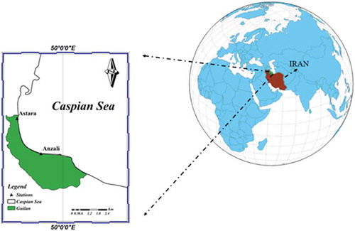
Table 1. Basic statistics of meteorological variables for Anzali station. SD: standard deviation; T: temperature; RH: relative humidity.

Parameter	Tmax	RHmax	RHmin	Rainfall	Wind speed	Sunshine hours	Pan evaporation
	(°C)	(%)	(%)	(mm/d)	(knot)	(h)	(mm/d)
Mean	19.5	92.5	73.1	4.8	6.7	5.3	2.8
SD	8.0	5.8	13.3	13.4	3.3	4.4	2.3
Skewness	–0.06	–2.28	–1.17	4.38	1.47	0.14	0.80
Max	36.0	100.0	100.0	128.9	27.0	13.8	10.1
Min	–0.2	30.0	10.0	0.0	0.0	0.0	0.0

Table 2. Basic statistics of meteorological variables for Astara station.

Parameter	Tmax	Tmin	Tmean	RHmax	RHmin	RHmean	Rainfall	Sunshine hours	Pan evaporation
	(°C)	(°C)	(°C)	(%)	(%)	(%)	(mm/d)	(h)	(mm/d)
Mean	19.6	12.3	15.9	92.6	63.6	78.1	3.4	5.2	2.5
SD	8.7	7.4	7.9	6.1	16.2	10.2	10.1	4.4	2.2
Skewness	–0.05	–0.16	–0.08	–2.16	–0.49	–0.78	5.50	0.21	0.97
Max	36.6	28.0	31.2	100.0	100.0	100.0	122.3	13.5	10.1
Min	–1.6	–7.8	–3.6	51.0	8.0	32.0	0.0	0.0	0.0

2.5 Error quantification

Four error measures were used to assess the performance of models in simulating the process of pan evaporation: (a) root mean square error (RMSE), which in our study has the unit of mm/d and shows the mean error of all estimates; (b) the coefficient of determination (R²), which is unitless and quantifies the linear dependence between estimated and observed pan evaporation data; (c) the Nash-Sutcliffe efficiency criterion (E), which is also unitless, varies from – ∞ to one and is an overall measure of model accuracy; and (d) the Willmott agreement index (WI; Willmott et al. 2012). The RMSE, R², E and WI are defined as follows, respectively:

(17) $\mathrm{R}\mathrm{M}\mathrm{S}\mathrm{E}=\sqrt{\frac{1}{m}{\sum }_{i=1}^m{\left(x_i-y_i\right)}^2}$(17)

(18) $R^2=\frac{{\left[{\sum }_{i=1}^m\left(x_i-\bar{x}\right)\left(y_i-\bar{y}\right)\right]}^2}{s_x^2{s}_y^2}$(18)

(19) $E=1-\frac{{\sum }_{i=1}^m{\left(x_i-y_i\right)}^2}{{\sum }_{i=1}^m{\left(x_i-\bar{x}\right)}^2}$(19)

(20) $\mathrm{W}\mathrm{I}=1-\frac{{\sum }_{i=1}^m\left|x_i-y_i\right|}{2{\sum }_{i=1}^m\left|x_i-\bar{x}\right|}$(20)

where x_i and y_i are, respectively, the ith observed data and its estimate; $\bar{x}$ and $\bar{y}$ are, respectively, the observed and estimated means; $s_x^2$ and $s_y^2$ are, respectively, the observed and estimated variances; and m is the total number of observed data.

3 Modelling results and discussion

3.1 Gamma test

As a primary step in the modelling, the gamma test (Stefánsson et al. 1997) was used to determine the relative importance of the nine input climatological variables. The results of the gamma test are tabulated in Table 3. First, the test was run by incorporating all the reported input variables and the gamma value (γ_all) was obtained. Then, a stepwise procedure was performed by eliminating the climatological variables one by one corresponding to the gamma test. It is expected that γ_all will be less than the other gamma values (γ); otherwise, it could be concluded that the dependent variable (daily pan evaporation) is not sensitive to the variable that is omitted from the input dataset. The V ratios presented in Table 3 are indicators of the degree of predictability of the given dependent variable (i.e. daily pan evaporation in this study). A V ratio equal to one means that the dependent variable follows a random process and cannot be estimated through the considered input vector. On the other hand, a V ratio close to zero (see Table 3) indicates a high degree of predictability of the dependent variable. The slope of the regression line (Table 3) indicates how complex is the function by which input variables are transformed into the dependent variable. According to the results of the gamma test presented in Table 3, eliminating minimum air temperature from the input vector of Anzali weather station decreases γ from 0.040 to 0.039 and increases the slope from 0.025 to 0.043 (the maximum slope), suggesting that daily pan evaporation is not sensitive to minimum temperature. Same conclusions can be made regarding mean air temperature and mean relative humidity. So, for this station, six variables – rainfall, maximum air temperature, maximum and minimum relative humidity (RH), actual sunshine hours and wind speed – were considered as the components of the input vector. In the case of Astara weather station, as eliminating wind speed from the input vector decreases γ from 0.040 to 0.039 and increases the slope to its maximum value (0.066), wind speed was omitted from the input dataset and the other eight variables were considered as independent variables for estimating daily pan evaporation.

Table 3. Gamma test results showing the relative importance of input meteorological variables. Bold indicates best fit. WS: wind speed; SH: sunshine hours; γ: gamma value.

Station	Removed variable	V ratio	Standard error	Slope of the regression line	γ
Anzali	-	0.160	0.0017	0.025	0.040
	Tmax	0.161	0.0008	0.029	0.041
	Tmin	0.155	0.0013	0.043	0.039
	Tmean	0.158	0.0010	0.033	0.039
	RHmax	0.160	0.0016	0.031	0.041
	RHmin	0.162	0.0006	0.024	0.041
	RHmean	0.154	0.0009	0.037	0.038
	Rainfall	0.167	0.0009	0.034	0.042
	WS	0.173	0.0019	0.019	0.043
	SH	0.188	0.0012	0.028	0.047
Astara	-	0.159	0.0006	0.035	0.040
	Tmax	0.161	0.0008	0.042	0.041
	Tmin	0.166	0.0009	0.032	0.042
	Tmean	0.164	0.0013	0.033	0.041
	RHmax	0.173	0.0009	0.019	0.043
	RHmin	0.166	0.0005	0.028	0.041
	RHmean	0.164	0.0012	0.029	0.041
	Rainfall	0.167	0.0014	0.041	0.042
	WS	0.158	0.0012	0.066	0.039
	SH	0.181	0.0010	0.063	0.045

3.2 MLP-KH modelling

Here, we present the evaluation of the proposed integration of artificial intelligence with a nature-inspired optimization algorithm (i.e. krill herd, KH) for evaporation process estimation. The modelling of the implemented MLP-KH is validated against a classical multiple layer perceptron (MLP) and support vector machine (SVM). Note that MLP and SVM models are predominantly used as data-intelligence for modelling the evaporation process (Bruton et al. 2000, Gavin and Agnew 2004, Shirsath and Singh 2010). Optimal values of the model parameters are presented in Table 4. Table 5 shows the performance metrics (R², RMSE, WI and E) for the testing phase. The proposed integrated model (MLP-KH) shows reasonable results with R² > 0.90, RMSE < 0.86, WI > 0.95 and E > 0.81 for both stations. The MLP-KH model shows also an augmentation over MLP and SVM, with 33–34% and 28–33% reduction in the value of RMSE over MLP and SVM models for Anzali and Astara stations, respectively.

Table 4. Optimal values of MLP, SVM and MLP-KH parameters for Anzali and Astara weather stations.

Parameter	Anzali			Astara
	MLP	SVM	MLP-KH	MLP	SVM	MLP-KH
Learning rate	0.001	–	–	0.001	–	–
Momentum	0.9	–	–	0.9	–	–
Number of initial input variables	9	9	9	9	9	9
Number of final input variables	6	6	6	8	8	8
Number of hidden layers	1	–	1	1	–	1
Number of nodes in hidden layer	17	–	17	11	–	11
Epoch (iteration)	1000	1000	1000	1000	1000	1000
Trade-off parameter, C	–	1.67	–	–	11.48	–
Radial basis function parameter, γ	–	0.1	–	–	1.1	–
Velocity of foraging	–	–	0.02	–	–	0.02
Maximum induced speed	–	–	0.01	–	–	0.01
Computational time (s)	18	24	28	17	23	26

Table 5. Statistical performance indicators for the MLP, SVM and MLP-KH models over the testing phase.

Station	Model	R^2	RMSE (mm/d)	WI	E
Anzali	MLP	0.792	1.088	0.942	0.789
	SVM	0.791	1.096	0.940	0.786
	MLP-KH	0.907	0.725	0.967	0.865
Astara	MLP	0.843	1.197	0.903	0.778
	SVM	0.803	1.290	0.891	0.742
	MLP-KH	0.931	0.855	0.950	0.813

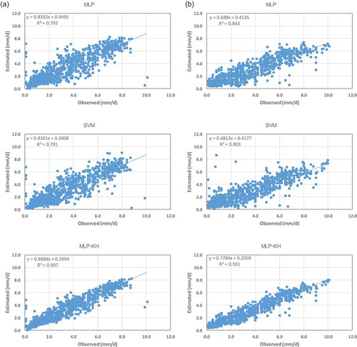
3.3 Scatter plot evaluation

Scatter plot is a very common technique used to evaluate the accuracy between actual and predicted values. As illustrated in Fig. 2(a) and (b), both stations performed well over the testing phase. However, it is seen that a few observed values are highly underestimated or overestimated. The proposed MLP-KH shows fewer scattered points from the diagonal line, suggesting that daily pan evaporation can be reliably predicted by the new integrated model over the classical ones. In more respective manners, considering the scatter plots and the calculated values for the Nash–Sutcliffe model efficiency coefficient (E), it is seen that MLP-KH produces more accurate estimates than that of MLP and SVM models.

Figure 2. Observed daily pan evaporation versus estimates produced by MLP, SVM and MLP-KH models over the testing phase: (a) Anzali station and (b) Astara station.

3.4 Taylor diagram, violin plot and point density distribution

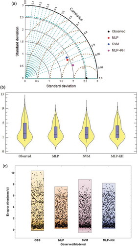
To show the prediction accuracy of the developed models, a graphical presentation using the Taylor diagram, violin plot and point density distribution over the testing phase is drawn and assessed for Anzali and Astara stations (Figs. 3 and 4, respectively). The Taylor diagram is a combination of three statistical performance metrics, RMSE, correlation coefficient and standard deviation (SD). A solid black circle represents the observed data and coloured circles show the modelling results. The RMSE is proportional to the distance between coloured and black circles. The correlation coefficient and the standard deviation are, respectively, related to the azimuthal angle of the coloured circle and its radial distance from the origin. The Taylor diagram visualizes the accuracy of the predictive models based on the distance between black (observed) and coloured (estimated) circles. The violin plot is a combination of a boxplot and a density plot of data. The Taylor plot in Fig. 3 shows that the developed and benchmark models for Anzali weather station have approximately the same SD. Furthermore, it is seen that for this station, all three models are quite well able to reproduce the observed SD value. In contrast, for Astara weather station (Fig. 4), the estimates produced by the models show little variability. The SD of MLP, SVM and MLP-KH models at Astara station over the testing phase was, respectively, 1.91, 1.92 and 2.05 mm/d, while the observed SD was 2.54 mm/d. In general, Figs. 3 and 4 suggest that, for both stations investigated in this research, the MLP-KH model performance gave the highest correlation coefficient and lowest RMSE over the testing phase and the results agree best with observations.

Figure 3. (a) Taylor diagram, (b) violin plot and (c) point density distribution to compare MLP, SVM and MLP-KH models with respect to the observed daily pan evaporation over the testing phase – Anzali weather station.

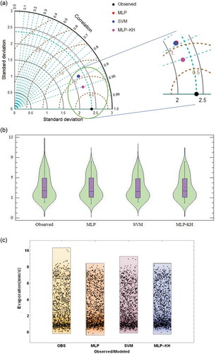
Figure 4. (a) Taylor diagram, (b) violin plot and (c) point density distribution to compare MLP, SVM and MLP-KH models with respect to the observed daily pan evaporation over the testing phase – Astara weather station.

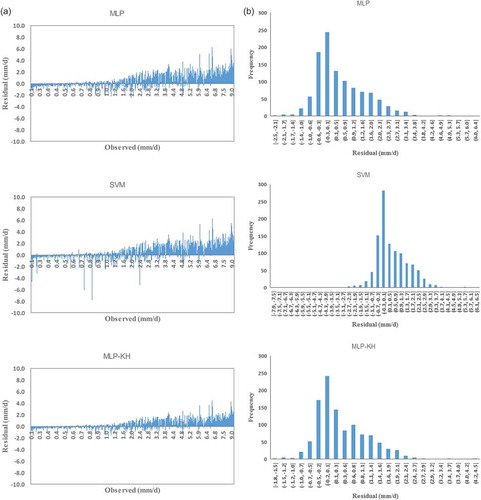
3.5 Residual analysis

Another evaluation of the estimated evaporation process is executed using residual analysis. The residual associated with each observed pan evaporation over the testing phase and the histograms of residuals are presented in Figs. 5 and 6 for Anzali and Astari, respectively. It is seen that at Anzali weather station (Fig. 5) and for all models, the histograms of residuals are symmetrical and near bell-shaped, suggesting that the residuals at this station follow a near normal distribution pattern with mean zero. In contrast, the histograms of Astara station (Fig. 6) are skewed and all models tend to underestimate daily pan evaporation. However, the mean of residuals for MLP, SVM and MLP-KH models were, respectively, 0.49, 0.51 and 0.35, showing that MLP-KH has the best fit.

Figure 5. (a) Residuals and (b) their distribution for MLP, SVM and MLP-KH models in estimating daily pan evaporation over the testing phase – Anzali weather station.

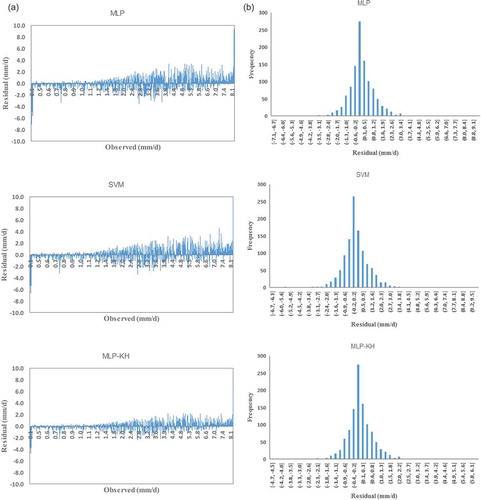
Figure 6. (a) Residuals and (b) their distribution for MLP, SVM and MLP-KH models in estimating daily pan evaporation over the testing phase – Astara weather station.

4 Conclusion

In this study, the feasibility of integrating a nature-inspired optimization algorithm with classical neural network models was investigated. Artificial neural networks are usually calibrated using optimization algorithms that are gradient-based, sometimes resulting in obtaining local optimal parameter sets. Although it is shown that nature-inspired optimization algorithms can be effectively used to calibrate neural network-based models, only a few studies have examined their possible capabilities in modelling hydrological variables. Here, to estimate daily pan evaporation in two weather stations located in northern Iran (namely Astara and Anzali), we introduced an integrated MLP-KH model (multilayer perceptron integrated with the krill herd optimization algorithm), which simultaneously benefits from the advantages of both ANNs and nature-inspired algorithms. Two benchmark model types, conventional MLPs and support vector machines were also developed and the proposed model was compared to them. To reduce the number of independent input variables of the ANN model, the gamma test was used. Reducing input variables resulted in fewer free parameters to be optimized. For one of the weather stations, the gamma test left out the wind speed independent variable from the input vector. Although wind speed is usually recognized as an important independent variable in evaporation estimation, the final modelling results showed that the estimates produced by the proposed model are quite exceptional. Different aspects of the models’ accuracy were assessed using Taylor diagrams, violin plots, point density distributions and residual analysis.

In the literature and in the field of using AI-based models to simulate the process of daily pan evaporation, different performances based on climatic conditions, number and type of climatological input variables and model type have been reported. For example, the coefficient of determination (R²) values over the testing phase (in the ranges 0.710–0.998, 0.423–0.925, 0.434–0.821, 0.504–0.704, 0.415–0.928, 0.479–0.883, 0.803–0.881 and 0.815–0.872) have been reported, respectively, by Kişi (2009) (best results obtained from MLP); Pammar and Deka (2017) (best results obtained from hybridization of wavelet transform and SVM); Deo and Samui (2017) (best results obtained from least square support vector regression, LS-SVR); Kisi et al. (2016) (best results obtained from MLP); Wang et al. (2017) (best results obtained from LS-SVR); Malik et al. (2018) (best results obtained from radial basis neural network, RBNN); Ashrafzadeh et al. (2018) (best results obtained from self-organizing feature map neural network) and Ghorbain et al. (2018) (best results obtained from MLP integrated with quantum-behaved particle swarm optimization algorithm). The above-mentioned R² values indicate that the results obtained in this study are quite reasonable (R² in the range 0.792–0.932).

Furthermore, a few studies have been tried to integrate bio-inspired algorithms (for example the firefly or particle swarm optimization algorithms) with neural networks for pan evaporation estimation. A disadvantage of the above-mentioned algorithms is that they use a set of parameters whose optimal values need to be determined using a meta-optimization technique, and the values selected for the parameters have large impacts on the optimization performance of the algorithm. Considering this, one can say that the krill herd algorithm has a major advantage over the other nature-inspired algorithms, and even over SVM.

The modelling results presented herein show that the KH-optimization algorithm can be used as an alternative to the conventional gradient descent optimization techniques to effectively optimize the parameters of a MLP network. It was observed that using the KH-optimization algorithm increased the accuracy of the estimates of daily pan evaporation produced by MLP or SVM models. The SVM has been predominantly applied for evaporation process simulation and had shown remarkable predictability performance. Hence, the SVM was selected for validating the proposed model in this study. According to the published review articles (e.g. Raghavendra and Deka 2014), SVM represents the most important development in the field of modelling hydrological parameters after fuzzy and artificial neural networks. However, while ANNs are sensitive to the number of hidden processing elements and the value of weight parameters, SVMs are mostly sensitive to the choice of kernel functions. So, the classical SVM was used for our study. However, the hypothesis that integrating SVM with the KH-optimization algorithm could improve the performance of SVM could be tested in future studies.

The results presented here collectively suggest that MLP-KH is a good choice to be used as an estimation model in our study area. Based on our results, it is concluded that the proposed model could be applicable to other hydrological variables. However, it should be mentioned that there is no definitive evidence for the superiority of a particular data-driven model, and the ability of a model in a specific region should be individually evaluated.

Acknowledgements

The authors wish to thank Iran Meteorological Organization for providing the data used in this study. We should also like to thank the reviewers and the editors who have given up valuable time to review the manuscript.

Disclosure statement

No potential conflict of interest was reported by the authors.

References

- Abghari, H., et al., 2012. Prediction of daily pan evaporation using wavelet neural networks. Water Resoures Management, 26 (12), 3639–3652. doi:10.1007/s11269-012-0096-z.
- Afan, H.A., et al., 2016. Past, present and prospect of an Artificial Intelligence (AI) based model for sediment transport prediction. Journal of Hydrology, 541, 902–913. doi:10.1016/j.jhydrol.2016.07.048
- Almedeij, J., 2012. Modeling pan evaporation for kuwait by multiple linear regression. The Scientific World Journal, 1–9. doi:10.1100/2012/574742.
- Ashrafzadeh, A., 1999. Application of artificial neural networks for prediction of evaporation from evaporative ponds. Thesis (M.Sc.). University of Tehran. (In Persian).
- Ashrafzadeh, A., et al., 2018. Estimation of daily pan evaporation using neural networks and meta-heuristic approaches. ISH Journal of Hydraulic Engineering, 1–9. doi:10.1080/09715010.2018.1498754.
- Boden, T.A., Krassovski, M., and Yang, B., 2013. The AmeriFlux data activity and data system: an evolving collection of data management techniques, tools, products and services. Geoscientific Instrumentation, Methods and Data Systems, 2 (1), 165–176. doi:10.5194/gi-2-165-2013.
- Bolaji, A.L., et al., 2016. A comprehensive review: krill herd algorithm (KH) and its applications. Applied Soft Computing, 49, 437–446. doi:10.1016/j.asoc.2016.08.041
- Bruton, J.M., McClendon, R.W., and Hoogenboom, G., 2000. Estimating daily pan evaporation with artificial neural networks. Transactions of the ASAE, 43 (2), 491–496. doi:10.13031/2013.2730.
- Carcano, E.C., et al., 2008. Jordan recurrent neural network versus IHACRES in modelling daily streamflows. Journal of Hydrology, 362 (3–4), 291–307. doi:10.1016/j.jhydrol.2008.08.026.
- Charalambous, C., 1992. Conjugate gradient algorithm for efficient training of artificial neural networks. IEE Proceedings G - Circuits, Devices and Systems, 139 (3), 301. doi:10.1049/ip-g-2.1992.0050.
- Chu, C.R., et al., 2010. A wind tunnel experiment on the evaporation rate of Class A evaporation pan. Journal of Hydrology, 381 (3–4), 221–224. doi:10.1016/j.jhydrol.2009.11.044.
- Clemence, B., 1987. Estimating class a pan evaporation at locations with sparse climatic data. South African Journal of Plant and Soil, 4 (3), 137–139. doi:10.1080/02571862.1987.10634960.
- Deo, R.C., et al., 2018. Multi-layer perceptron integrated model integrated with the firefly optimizer algorithm for windspeed prediction of target site using a limited set of neighboring reference station data. Renewable Energy, 116, 309–323. doi:10.1016/j.renene.2017.09.078
- Deo, R.C. and Samui, P., 2017. Forecasting evaporative loss by least-square support-vector regression and evaluation with genetic programming, gaussian process, and minimax probability machine regression: case study of Brisbane City. Journal of Hydrologic Engineering, 22, 6. doi:10.1061/(ASCE)HE.1943-5584.0001506
- Dogan, E., et al., 2010. Modelling of evaporation from the reservoir of Yuvacik dam using adaptive neuro-fuzzy inference systems. Engineering Applications of Artificial Intelligence, 23 (6), 961–967. doi:10.1016/j.engappai.2010.03.007.
- Fitzpatrick, E.A., 1963. Estimates of pan evaporation from mean maximum temperature and vapour pressure. Journal of Applied Meteorology and Climatology, 2, 6. doi:10.1175/1520-0450(1963)002<0780:EOPEFM>2.0.CO;2
- Fombellida, M. and Destiné, J., 1992. The extended quickprop. Proceedings of the 1992 International Conference on Artificial Neural Networks, 973–977. doi:10.1016/B978-0-444-89488-5.50032-4
- Gallego-Elvira, B., et al., 2012. Evaluation of evaporation estimation methods for a covered reservoir in a semi-arid climate (south-eastern Spain). Journal of Hydrology, 458–459, 59–67. doi:10.1016/j.jhydrol.2012.06.035
- Gandomi, A.H. and Alavi, A.H., 2012. Krill herd: A new bio-inspired optimization algorithm. Communications in Nonlinear Science and Numerical Simulation, 17 (12), 4831–4845. doi:10.1016/j.cnsns.2012.05.010.
- Gavin, H. and Agnew, C.A., 2004. Modelling actual, reference and equilibrium evaporation from a temperate wet grassland. Hydrological Processes, 18 (2), 229–246. doi:10.1002/hyp.1372.
- Ghorbani, M.A., et al., 2017a. Pan evaporation prediction using a hybrid multilayer perceptron-firefly algorithm (MLP-FFA) model: case study in North Iran. Theoretical and Applied Climatology, 133 (3–4), 1119–1131. doi:10.1007/s00704-017-2244-0.
- Ghorbani, M.A., et al., 2017b. Application of firefly algorithm-based support vector machines for prediction of field capacity and permanent wilting point. Soil and Tillage Research, 172, 32–38. doi:10.1016/J.STILL.2017.04.009
- Ghorbani, M.A., et al., 2018. Forecasting pan evaporation with an integrated artificial neural network quantum-behaved particle swarm optimization model : a case study in Talesh, Northern Iran. Engineering Applications of Computational Fluid Mechanics, 12 (1), 724–737. doi:10.1080/19942060.2018.1517052.
- Goyal, M.K., et al., 2014. Modeling of daily pan evaporation in sub tropical climates using ANN, LS-SVR, Fuzzy Logic, and ANFIS. Expert Systems with Applications, 41 (11), 5267–5276. doi:10.1016/j.eswa.2014.02.047.
- Hadinia, H., Pirmoradian, N., and Ashrafzadeh, A., 2017. Effect of changing climate on rice water requirement in guilan, north of Iran. Journal of Water and Climate Change, 8, 1. doi:10.2166/wcc.2016.025
- Hagan, M.T. and Menhaj, M.B., 1994. Training feedforward networks with the Marquardt algorithm. IEEE Transactions on Neural Networks, 5 (6), 989–993. doi:10.1109/72.329697.
- Hofmann, E.E., et al., 2004. Lagrangian modelling studies of Antarctic krill (Euphausia superba) swarm formation. ICES Journal of Marine Science, 61, 617–631. doi:10.1016/j.icesjms.2004.03.028
- Jacobs, R.A., 1988. Increased rates of convergence through learning rate adaptation. Neural Networks, 1 (4), 295–307. doi:10.1016/0893-6080(88)90003-2.
- Jensi, R. and Jiji, G.W., 2016. An improved krill herd algorithm with global exploration capability for solving numerical function optimization problems and its application to data clustering. Applied Soft Computing, 46, 230–245. doi:10.1016/J.ASOC.2016.04.026
- Keskin, M.E. and Terzi, Ö., 2006. Artificial neural network models of daily pan evaporation. Journal of Hydrologic Engineering, 11 (1), 65. doi:10.1061/(ASCE)1084-0699(2006)11:1(65).
- Keskin, M.E., Terzi, Ö., and Taylan, D., 2009. Estimating daily pan evaporation using adaptive neural-based fuzzy inference system. Theoretical and Applied Climatology, 98 (1–2), 79–87. doi:10.1007/s00704-008-0092-7.
- Kim, S. and Kim, H.S., 2008. Neural networks and genetic algorithm approach for nonlinear evaporation and evapotranspiration modeling. Journal of Hydrology, 351 (3–4), 299–317. doi:10.1016/J.JHYDROL.2007.12.014.
- Kişi, Ö., 2006. Daily pan evaporation modelling using a neuro-fuzzy computing technique. Journal of Hydrology, 329 (3–4), 636–646. doi:10.1016/j.jhydrol.2006.03.015.
- Kişi, Ö., 2009. Daily pan evaporation modelling using multi-layer perceptrons and radial basis neural networks. Hydrological Processes, 23 (2), 213–223. doi:10.1002/hyp.7126.
- Kişi, Ö., et al., 2016. Daily pan evaporation modeling using chi-squared automatic interaction detector, neural networks, classification and regression tree. Computers and Electronics in Agriculture, 122, 112–117. doi:10.1016/j.compag.2016.01.026
- Kowalski, P.A. and Łukasik, S., 2016. Training neural networks with krill herd algorithm. Neural Processing Letters, 44 (1), 5–17. doi:10.1007/s11063-015-9463-0.
- Lim, W.H., et al., 2012. The aerodynamics of pan evaporation. Agricultural and Forest Meteorology, 152 (1), 31–43. doi:10.1016/j.agrformet.2011.08.006.
- Lim, W.H., Roderick, M.L., and Farquhar, G.D., 2016. A mathematical model of pan evaporation under steady state conditions. Journal of Hydrology, 540, 641–658. doi:10.1016/j.jhydrol.2016.06.048
- Maier, H.R. and Dandy, G.C., 2000. Neural networks for the prediction and forecasting of water resources variables: a review of modelling issues and applications. Environmental Modelling and Software, 15 (1), 101–124. doi:10.1016/S1364-8152(99)00007-9.
- Malik, A. and Kumar, A., 2015. Pan evaporation simulation based on daily meteorological data using soft computing techniques and multiple linear regression. Water Resources Management, 29 (6), 1859–1872. doi:10.1007/s11269-015-0915-0.
- Malik, A., Kumar, A., and Kişi, Ö., 2017. Monthly pan-evaporation estimation in Indian central Himalayas using different heuristic approaches and climate based models. Computers and Electronics in Agriculture, 143, 302–313. doi:10.1016/j.compag.2017.11.008
- Malik, A., Kumar, A., and Kişi, Ö., 2018. Daily pan evaporation estimation using heuristic methods with Gamma test. Journal of Irrigation and Drainage Engineering, 144, 9. doi:10.1061/(ASCE)IR.1943-4774.0001336
- Mandal, B., Roy, P.K., and Mandal, S., 2014. Economic load dispatch using krill herd algorithm. International Journal of Electrical Power and Energy Systems, 57, 1–10. doi:10.1016/J.IJEPES.2013.11.016
- Mizoguchi, Y., et al., 2009. A review of tower flux observation sites in Asia. Journal of Forestry Research, 14 (1), 1–9. doi:10.1007/s10310-008-0101-9.
- Molina Martínez, J.M., et al., 2006. A simulation model for predicting hourly pan evaporation from meteorological data. Journal of Hydrology, 318 (1–4), 250–261. doi:10.1016/j.jhydrol.2005.06.016.
- Moodley, K., Rarey, J., and Ramjugernath, D., 2015. Application of the bio-inspired Krill Herd optimization technique to phase equilibrium calculations. Computers and Chemical Engineering, 74, 75–88. doi:10.1016/J.COMPCHEMENG.2014.12.008
- Mukherjee, A., Roy, P.K., and Mukherjee, V., 2016. Transient stability constrained optimal power flow using oppositional krill herd algorithm. International Journal of Electrical Power and Energy Systems, 83, 283–297. doi:10.1016/J.IJEPES.2016.03.058
- Nourani, V. and Sayyah Fard, M., 2012. Sensitivity analysis of the artificial neural network outputs in simulation of the evaporation process at different climatologic regimes. Advances in Engineering Software, 47 (1), 127–146. doi:10.1016/j.advengsoft.2011.12.014.
- Pammar, L. and Deka, P.C., 2017. Daily pan evaporation modeling in climatically contrasting zones with hybridization of wavelet transform and support vector machines. Paddy and Water Environment, 15 (4), 711–722. doi:10.1007/s10333-016-0571-x.
- Piri, J., et al., 2009. Daily pan evaporation modeling in a hot and dry climate. Journal of Hydrologic Engineering, 14 (8), 803–811. doi:10.1061/(ASCE)HE.1943-5584.0000056.
- Raghavendra, S. and Deka, P.C., 2014. Support vector machine applications in the field of hydrology: A review. Applied Soft Computing Journal, 19, 372–386. doi:10.1016/j.asoc.2014.02.002
- Rahimikhoob, A., 2009. Estimating daily pan evaporation using artificial neural network in a semi-arid environment. Theoretical and Applied Climatology, 98 (1–2), 101–105. doi:10.1007/s00704-008-0096-3.
- Rotstayn, L.D., Roderick, M.L., and Farquhar, G.D., 2006. A simple pan-evaporation model for analysis of climate simulations: evaluation over Australia. Geophysical Research Letters, 33 (17), 1–5. doi:10.1029/2006GL027114.
- Rumelhart, D.E., Hinton, G.E., and Williams, R.J., 1986. Learning representations by back-propagating errors. Nature, 323 (6088), 533–536. doi:10.1038/323533a0.
- Shirsath, P.B. and Singh, A.K., 2010. A comparative study of daily pan evaporation estimation using ANN, regression and climate based models. Water Resources Management, 24 (8), 1571–1581. doi:10.1007/s11269-009-9514-2.
- Singh, V.P. and Xu, C.-Y., 1997. Evaluation and generalization of 13 mass-transfer equations for determining free water evaporation. Hydrological Processes, 11, 311–323. doi:10.1002/(SICI)1099-1085(19970315)11:3<311::AID-HYP446>3.3.CO;2-P
- Stanhill, G., 2002. Is the class A evaporation pan still the most practical and accurate meteorological method for determining irrigation water requirements?. Agricultural and Forest Meteorology, 112 (3–4), 233–236. doi:10.1016/S0168-1923(02)00132-6.
- Stasinakis, C., et al., 2016. Krill-Herd Support Vector Regression and heterogeneous autoregressive leverage: evidence from forecasting and trading commodities. Quantitative Finance, 16 (12), 1901–1915. doi:10.1080/14697688.2016.1211800.
- Stefánsson, A., Končar, N., and Jones, A., 1997. A note on the gamma test. Neural Computing and Applications, 5 (3), 131–133. doi:10.1007/BF01413858.
- Sudheer, K.P., et al., 2002. Modelling evaporation using an artificial neural network algorithm. Hydrological Processes, 16 (16), 3189–3202. doi:10.1002/hyp.1096.
- Sultana, S. and Roy, P.K., 2016. Krill herd algorithm for optimal location of distributed generator in radial distribution system. Applied Soft Computing, 40, 391–404. doi:10.1016/J.ASOC.2015.11.036
- Sun, S., et al., 2016. Inverse geometry design of two-dimensional complex radiative enclosures using krill herd optimization algorithm. Applied Thermal Engineering, 98, 1104–1115. doi:10.1016/J.APPLTHERMALENG.2016.01.017
- Tabari, H., Marofi, S., and Sabziparvar, A.A., 2010. Estimation of daily pan evaporation using artificial neural network and multivariate non-linear regression. Irrigation Science, 28 (5), 399–406. doi:10.1007/s00271-009-0201-0.
- Tan, S.B.K., Shuy, E.B., and Chua, L.H.C., 2007. Modelling hourly and daily open-water evaporation rates in areas with an equatorial climate. Hydrological Processes, 21 (4), 486–499. doi:10.1002/hyp.6251.
- Valentini, R., et al., 2000. Respiration as the main determinant of carbon balance in European forests. Nature, 404 (6780), 861–865. doi:10.1038/35009084.
- Vapnik, V., Golowich, S.E., and Smola, A., 1996. Support vector method for function approximation, regression estimation, and signal rrocessing. Annual Conference on Neural Information Processing Systems, 281–287. doi:10.1007/978-3-642-33311-8_5
- Wang, G.G., et al., 2019. A comprehensive review of krill herd algorithm: variants, hybrids and applications. Artificial Intelligence Review, 51 (1), 119–148. doi:10.1007/s10462-017-9559-1.
- Wang, L., et al., 2017. Pan evaporation modeling using four different heuristic approaches. Computers and Electronics in Agriculture, 140, 203–213. doi:10.1016/j.compag.2017.05.036
- Willmott, C.J., Robeson, S.M., and Matsuura, K., 2012. A refined index of model performance. International Journal of Climatology, 32 (13), 2088–2094. doi:10.1002/joc.2419.
- Wu, W., Dandy, G.C., and Maier, H.R., 2014. Protocol for developing ANN models and its application to the assessment of the quality of the ANN model development process in drinking water quality modelling. Environmental Modelling and Software, 54, 108–127. doi:10.1016/j.envsoft.2013.12.016
- Xiong, A.Y., Liao, J., and Xu, B., 2012. Reconstruction of a daily large-pan evaporation dataset over China. Journal of Applied Meteorology and Climatology, 51 (7), 1265–1275. doi:10.1175/JAMC-D-11-0123.1.
- Xu, C.-Y. and Singh, V.P., 2000. Evaluation and generalization of radiation-based methods for calculating evaporation. Hydrological Processes, 14 (2), 339–349. doi:10.1002/(SICI)1099-1085(20000215)14:2<339::AID-HYP928>3.0.CO;2-O.
- Yaseen, Z.M., et al., 2015. Artificial intelligence based models for stream-flow forecasting: 2000–2015. Journal of Hydrology, 530, 829–844. doi:10.1016/j.jhydrol.2015.10.038
- Yaseen, Z.M., et al., 2017. Novel approach for streamflow forecasting using a hybrid ANFIS-FFA model. Journal of Hydrology, 554, 263–276. doi:10.1016/j.jhydrol.2017.09.007.