Simple stochastic simulation of time irreversible and reversible processes

ABSTRACT

As time irreversibility of streamflow is marked for time scales up to several days, while common stochastic generation methods are good only for time-symmetric processes, the need for new methods to handle irreversibility, particularly in flood simulations, has been recently highlighted. From an investigation of the historical evolution of existing stochastic generation methods, which is a useful step before proposing new methods, the strengths and weaknesses of current approaches are located. Following this investigation, a generic solution to the stochastic generation problem is proposed. This is an analytical exact method based on an asymmetric moving-average scheme, capable of handling time irreversibility in addition to preserving the second-order stochastic structure, as well as higher-order marginal statistics, of a process. The method is studied theoretically in its general setting, as well as in its most interesting special cases, and is successfully applied to streamflow generation at an hourly scale.

KEYWORDS:

• time’s arrow
• irreversibility
• stochastic simulation
• time series
• Monte Carlo method

Editor A. CastellarinAssociate editor not assigned

1 Introduction

Simplicity is the final achievement.

Frédéric Chopin

A recent study (Koutsoyiannis 2019b) has investigated the possible existence of time irreversibility in hydrometeorological processes and the related theoretical framework. According to the latter, a simple definition of time reversibility within stochastics is the following, where underlined symbols denote stochastic (random) variables and non-underlined ones denote values thereof or regular variables.

A stochastic process $\underset{\_}{x}(t)$ at continuous time t, with nth order distribution function:

(1) $F\left(x_1,x_2,\dots ,x_n;t_1,t_2,\dots ,t_n\right):=P\left\{\underset{\_}{x}\left(t_1\right)\le x_1,\underset{\_}{x}\left(t_2\right)\le x_2,\dots ,\underset{\_}{x}\left(t_n\right)\le x_n\right\}$(1)

is time-symmetric or time-reversible if its joint distribution does not change after reflection of time about the origin, i.e. if for any n, $t_1,t_2,\dots ,t_n$,

(2) $\begin{array}{rl}& F\left(x_1,x_2,\dots ,x_n;t_1,t_2,\dots ,t_n\right)\\ & =F\left(x_1,x_2,\dots ,x_n;-t_1,-t_2,\dots ,-t_n\right)\end{array}$(2)

If times $t_i$ are equidistant, i.e. $t_i-t_{i-1}=D$, the definition can be also written by reflecting the order of points in time, i.e.:

(3) $\begin{array}{rl}& F\left(x_1,x_2,\dots ,x_{n-1},x_n;t_1,t_2,\dots ,t_{n-1},t_n\right)\\ & =F\left(x_1,x_2,\dots ,x_{n-1},x_n;t_n,t_{n-1},\dots ,t_2,t_1\right)\end{array}$(3)

A process that is not time-reversible is called time-asymmetric, time-irreversible or time-directional. Important results related to time (ir)reversibility are the following:

• A time-reversible process is also stationary (Lawrance 1991).

• If a scalar process $\underset{\_}{x}(t)$ is Gaussian (i.e. all its finite-dimensional distributions are multivariate normal) then it is reversible (Weiss 1975). The consequences are: (a) a directional process cannot be Gaussian; (b) a discrete-time ARMA process (and a continuous-time Markov process) is reversible if and only if it is Gaussian.

• However, a vector (multivariate) process can be Gaussian and irreversible at the same time. A multivariate Gaussian linear process is reversible if and only if its autocovariance matrices are all symmetric (Tong and Zhang 2005).

Time asymmetry of a process can be studied through the differenced process, i.e.:

(4) ${\underset{\_}{\tilde{x}}}_{\tau }:={\underset{\_}{x}}_{\tau }-{\underset{\_}{x}}_{\tau -1}$(4)

where ${\underset{\_}{x}}_{\tau }$ is the process representation in discrete time τ (denoting the continuous-time interval $\left[\left(\tau -1\right)D,\tau D\right]$), i.e.:

(5) ${\underset{\_}{x}}_{\tau }:=\frac{1}{D}{\displaystyle \underset{\left(\tau -1\right)D}{\overset{\tau D}{\int }}\underset{\_}{x}}\left(u\right)\text{d}u$(5)

For a stationary stochastic process $\underset{\_}{x}(t)$, the differenced process ${\underset{\_}{\tilde{x}}}_{\tau }$ has mean zero and variance:

(6) ${\tilde{\gamma }}_1:=var\left[{\underset{\_}{\tilde{x}}}_{\tau }\right]=2\left({\gamma }_1-c_1\right)$(6)

where ${\gamma }_1$ and $c_1$ are the variance and lag-one autocovariance, respectively, of ${\underset{\_}{x}}_{\tau }$. Then, the time asymmetry is quantified by the skewness coefficient:

(7) ${\tilde{C}}_{\mathrm{S}}:=\frac{{\mu }_3\left[{\underset{\_}{\tilde{x}}}_{\tau }\right]}{{\left(var\left[{\underset{\_}{\tilde{x}}}_{\tau }\right]\right)}^{3/2}}$(7)

where ${\mu }_3\left[\right]$ denotes the third moment. Alternatively, it is quantified by the probability of ${\underset{\_}{\tilde{x}}}_{\tau }$ being negative:

(8) ${\tilde{P}}_{\mathrm{N}}:=P\left\{{\underset{\_}{\tilde{x}}}_{\tau }\le 0\right\}={\tilde{F}}_{{\underset{\_}{\tilde{x}}}_{\tau }}\left(0\right)$(8)

Processes with large ${\tilde{C}}_{\mathrm{S}}$ or large departure of ${\tilde{P}}_{\mathrm{N}}$ from the value 1/2 signify high (positive) time irreversibility. A sketch of a realization of such a process is given in Fig. 1. The graph is characterized by rapid increases followed by gradual decreases. The entire setting in constructing the time series of Fig. 1 is nonlinear (the values are obtained by optimization rather than generated by a linear stochastic model), and while the marginal distribution is by construction Gaussian, the multivariate one is not, so there is no conflict with Weiss’s (1975) result mentioned above.

The study by Koutsoyiannis (2019b) has provided evidence that time irreversibility may be profound in the streamflow process at scales of several days or lower. In atmospheric processes irreversibility appears as well, but at much finer time scales. On the other hand, most stochastic simulation methods do not account for irreversibility. In the same study, two methods have been proposed for a stochastic generation that respects irreversibility and reproduces it in a controlled manner, quantifying it by the skewness of the differenced process. After exploring them, one of the two methods proved successful. A disadvantage of that method is that it needs iterations to converge to a solution, in which vector derivatives need to be evaluated.

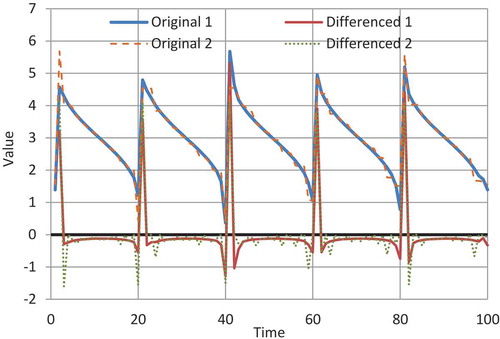
Figure 1. Plot of two synthetic time series generated by maximizing time irreversibility properties of a process restricted to be marginally Gaussian (N(3, 1)) with lag-one autocorrelation 0.5, so that the variance of the differenced process is also 1 (equal to that of the original process). Solution 1 maximizes the skewness of the differenced process. Solution 2 maximizes the frequency that the differenced process has a negative value, without taking into account the skewness. In both series the frequency that the differenced process has negative values is 0.94. The coefficients of skewness of the differenced processes for series 1 and 2 are 4.10 and 3.34, respectively (Source: Koutsoyiannis 2019b).

Here we present a simple method that is exact, analytical and direct, and its application is fast avoiding the need for iterations. As far as the general framework related to time’s arrow and time irreversibility of atmospheric and hydrological processes is concerned, the interested reader is referred to the study by Koutsoyiannis (2019b) and its extended list of references. However, in terms of the stochastic synthesis per se, the current paper is a stand-alone study with a detailed presentation, starting from main historical landmarks and ending with proposing a generic method of stochastic synthesis which is entirely new (to the author’s knowledge). In this manner, an earlier study for a generic and parsimonious stochastic modelling scheme (Koutsoyiannis 2016) is complemented and extended to time-irreversible processes.

2 Approaches in stochastic synthesis

It is common knowledge that when we want to model the (marginal) distribution of a stochastic variable, we usually fit a model (a distribution such as Gaussian, gamma, generalized extreme value, etc.) using the available data, typically given as a time series $x_n,n=1,\dots ,N$. But let us consider for a minute a different tactic: We estimate from the data sufficiently many, say J, moments, and instead of fitting a customary distribution, we approximate the distribution through moments. These moments are ${{\displaystyle \mu }}_j^{´}:=\text{E}\left[{\underset{\_}{x}}^j\right],j=1,2,\dots ,J$, and their unbiased estimates from the data are ${\hat{\mu }}_j^{\prime }:={\sum }_{n=1}^N{x}_n^j/N$. From the moments we could recover the density function $f\left(x\right)$ of the stochastic variable of interest $\underset{\_}{x}$, in at least two ways:

1.We could exploit the inversion formula (e.g. Papoulis 1991, p. 116):

(9) $f\left(x\right)=\frac{1}{2\pi }\underset{-\mathrm{\infty }}{\overset{\mathrm{\infty }}{\int }}\phi \left(\omega \right){\mathrm{e}}^{-\mathrm{i}\omega x}\mathrm{d}\omega$(9)

where $\phi \left(\omega \right)$ is the characteristic function of the distribution and $\mathrm{i}:=\sqrt{-1}$ is the imaginary unit, combine it with the moment theorem, according to which the jth derivative of $\phi \left(\omega \right)$ is:

(10) ${\phi }^{\left(j\right)}\left(\omega \right)={\mathrm{i}}^j{\mu }_j^{\prime }$(10)

and then use some type of expansion to approximate $\phi \left(\omega \right)$ and eventually $f\left(x\right)$ based on a number J of moment estimates.

2.We could use as an approximation of $f\left(x\right)$ the maximum entropy distribution conditional on the specified moments, which is (e.g. Papoulis 1991, p. 571):

(11) $f\left(x\right)=exp\left(\sum _{j=0}^J{\lambda }_j{x}^j\right)$(11)

where ${\lambda }_j$ are constants determined so that the distribution have the specified moments.

This tactic, if implemented in either variant, would have problems, including the following:

• Assuming that the number J is not very small, the resulting models would not be parsimonious, as they would include J moments and an equal number of parameters.

• The moment estimates beyond second are unreliable for typical sample sizes, despite the fact that unbiasedness is theoretically guaranteed (see the work by Lombardo et al. 2014, with the characteristic title “Just two moments”.)

• In particular, heavy-tailed distributions would never appear as models, because in these distributions all moments beyond a threshold are infinite, while their sample estimates are finite.

The origin of problems in such a tactic is not actually the approximate character of the specified distribution – after all, any model is an approximation of some real phenomenon. Rather, it is the lack of parsimony and the direct link of the parameters (such as ${\lambda }_j$ in (11)) with the data, on which their estimation is based. In contrast, the same approximation of the distribution would be valid and not problematic if coefficients ${\lambda }_j$ were not model parameters and if they were determined theoretically rather than estimated from the data.

Fortunately, however, this tactic is not commonly implemented. Rather, a parametric model is assumed based, on the one hand, on some theoretical considerations (e.g. central limit theorem, maximum entropy principle, asymptotic theory of distribution of extremes) and on the other hand, on some exploration of the available data.

Strangely enough though, this tactic has been the rule in fitting and applying so-called time-series models – and it is still the norm even today – despite the fact that fitting a stochastic process is more demanding a task than fitting a marginal distribution and, at the same time, the presence of autocovariance increases uncertainty in model fitting. Indeed, time-series models are typically fitted based on estimates of the autocovariance (or autocorrelation) function and even the model formulation (in terms of the multivariate distribution) is determined by the number of the autocorrelation coefficients they are used – similar to what Eq. (11) suggests for the marginal distribution. Apparently, the alternative of fitting a parametric model to the multivariate distribution is valid (Koutsoyiannis 2000, 2016) but it has not been the norm. The reasons for following such a weird practice in most disciplines whose modelling relies on data, including hydrology, are historical. An attempt to trace their evolution is contained in the next section.

3 A historical overview of stochastic modelling

Current stochastic modelling practices have been influenced by at least three Schools of thought, which will be referred to as (a) the Stochastic School, (b) the Time Series School and (c) the Monte Carlo School. We attempt to trace out the evolution in each of them in the next subsections, while an individual subsection is devoted to hydrology.

3.1 The Stochastic School

Perhaps Ludwig Boltzmann (1844–1906, Universities of Graz and Vienna, Austria, and Munich, Germany) was the first to introduce fundamental concepts related to stochastic process. In particular, Boltzmann (1877) explained the concept of entropy in probability theoretic context and Boltzmann (1884/85) introduced the notion of ergodic systems,¹ which is central in stochastics. Later George D. Birkhoff (1884–1944; Princeton, Harvard, USA) discovered the ergodic theorem (Birkhoff 1931) also known as the Birkhoff–Khinchin theorem to give credit to Aleksandr Khinchin (also spelt Khintchine, 1894–1959; Moscow State University, Russia), who gave a purely measure-theoretic proof of the theorem (Khintchine 1933). In addition, Khintchine (1934) defined the stationary stochastic processes and introduced a probabilistic setting of the Wiener-Khinchin theorem relating autocovariance and power spectrum.

But it was Andrey N. Kolmogorov (1903–1987; Moscow State University, Russia), the great scientist who founded the stochastic theory. Kolmogorov (1931) introduced the term stochastic process,² identifying process with change. He also used the term stationary to describe a probability density function that is unchanged in time. Kolmogorov (1933) defined probability (founded on measure theory) in an axiomatic manner based on three fundamental concepts (a triplet called probability space) and four axioms (non-negativity: normalization, additivity and continuity at zero). Kolmogorov (1937, 1938) gave a concise presentation of the concept of a stationary stochastic process and Kolmogorov (1947) defined wide-sense stationarity.

The concept of stationarity (and its negation, nonstationarity) has a central role in stochastics yet is widely misunderstood and broadly misused (Montanari and Koutsoyiannis 2014, Koutsoyiannis and Montanari 2015). Stationarity is tightly connected to ergodicity, which in turn is a prerequisite to make inference from data, that is, induction. If a system that is modelled in a stochastic framework has deterministic dynamics then it is stationary if it is ergodic and vice versa (Mackey 2003, p. 52). Likewise, a nonstationary system is also non-ergodic and vice versa. If the system dynamics is stochastic, then ergodicity and stationarity do not necessarily coincide. However, recalling that a stochastic process is a model (not part of the real world), we can always devise a stationary stochastic process that is ergodic.

It may be useful to include here a reminder of the definitions of the two concepts. Following Kolmogorov (1931, 1938) and Khintchine (1934), a process is stationary if its statistical properties are invariant to a shift of time origin, i.e. the processes $\underset{\_}{x}\left(t\right)$ and $\underset{\_}{x}\left(t^{\prime }\right)$ have the same (multivariate) distribution for any t and t΄. Based on the ergodic theorem (Birkhoff 1931, Khintchine 1933; see also Mackey 2003, p. 54), a stochastic process $\underset{\_}{x}\left(t\right)$ is ergodic if the time average of any (integrable) function g(x(t)), as time tends to infinity, equals the true (ensemble) expectation, i.e.:

(12) $\underset{T\to \infty }{\lim }\frac{1}{T}{\displaystyle \underset{0}{\overset{T}{\int }}g}\left(\underset{\_}{x}\left(t\right)\right)dt=\text{E}\left[g\left(\underset{\_}{x}\left(t\right)\right)\right]$(12)

3.2 The Time Series School

Contrary to the theoretical Stochastic School, the Time Series School is more intuitive and empirical, and less rigorous. Its history was written more by economists and less by theoretical mathematicians. Perhaps the first who introduced time-series analysis was the American economist W.M. Persons. In studying the problem “When to buy or sell”, Persons (1919) introduced the study of time series, which he called statistical series, and asserted that they “result from the combination of four elements: secular trend, seasonal variation, cyclical fluctuation, and a residual factor.” He also proposed methods for “Eliminating secular trends” and “Eliminating seasonal variation”. A definition of a time series was given 10 years later by the American statistician Bailey (1929): “A time series is a series of observations taken at different times and recorded with the time at which they were taken.”

Interestingly, Slutsky (1927) demonstrated that what Persons (and other economists) regarded as a cyclical component is nothing but a statistical artefact with no essential meaning (see e.g. Kyun and Kim 2006, Barnett 2006). Subsequently, the notion of a cyclical component was abandoned but the decomposition of a time series to the remaining three components, trends, seasonal variation and residuals is popular even today.

Yule (1927) and Walker (1931) (both British statisticians), starting from an analysis of sunspot numbers, studied autoregressive processes and in particular their periodogram and autocorrelation properties. But the biggest progress in the Time Series School was made in Uppsala by H.O.A. Wold (a Norwegian-born econometrician and statistician with a career in Sweden) and P. Whittle (a New-Zealand-born mathematician and statistician), who, in their doctoral theses, provided the stochastic foundation of time-series analysis. Wold (1938, 1948) proved that a stochastic process (even though he referred to it as a time series) can be decomposed into a regular process (i.e. a process linearly equivalent to a white noise process) and a predictable process (i.e. a process that can be expressed in terms of its past values). Whittle (1951, 1952, 1953) laid the mathematical foundation of autoregressive and moving-average models in univariate and multivariate setting. Later, in their influential book, Box and Jenkins (1970) named these models with acronyms such as AR(p) (autoregressive models of order p), MA(q) (moving average models of order q), ARMA(p,q) (autoregressive moving-average models) and ARIMA(p,d,q) (autoregressive integrated moving-average models). These became popular under these names and have also been known as Box–Jenkins models (cf. Stigler’s law of eponymy; Stigler 2002). A useful extension of these models to apply to processes with long-range dependence was proposed by Hosking (1981). This is done by replacing the integer parameter d in ARIMA(p,d,q) with a real one (fractional differencing) and the models are usually termed ARFIMA(p,d,q).

Despite the wider influence of the Time Series School over the Stochastic School, there are several problems with the former. First, the term time series is ambiguous, sometimes denoting a series of observations, as in the original definition of Bailey (1929) (or, equivalently, a realization of a stochastic process), and at other times denoting the stochastic process per se, as in the aforementioned use by Wold. We emphasize that here the term time series is used with the first meaning, a series of numbers, while for a series of random variables we use the term stochastic process. Second, with the exception of the simplest models of these families, such as the AR(1) and ARMA(1,1), time-series models are too artificial because, being complicated discrete-time models, they do not necessarily correspond to a continuous-time process, while natural processes typically evolve in continuous time. Furthermore, their identification, typically based on the estimation of the autocorrelation function from data, usually neglects estimation bias and uncertainty, which in stochastic processes (as opposed to purely random processes) are often tremendous (Lombardo et al. 2014).

Indeed, from their onset, time-series models have been tightly associated with a large number of parameters and they usually become over-parameterized and thus not parsimonious. These parameters are estimated from data, which usually are too few to support a reliable estimation. In Whittle’s (1952) words (emphasis added):

There is, of course, nothing special with the autoregressive scheme; we could equally well graduate with a high-order moving average, and there are many other possibilities. […] In practice, however, the autoregressive graduation has the advantage that the estimated residual sum of squares can be written down directly in terms of the observations […] without the need to solve explicitly for the estimates of the ‘a’ coefficients.

…

It is, of course, not possible to estimate an infinite number of parameters from a finite sample, but the series of a coefficients must converge, and by considering sufficiently many coefficients we should be able to obtain an arbitrarily good approximation to the real process.

This is similar to fitting a distribution function using observations to estimate many moments as described in Sec. 2.

The decomposition of a time series to components, trends, seasonal variation and residuals is fundamentally problematic, despite being popular. (In particular trend analysis of hydroclimatic processes is more fashionable today than ever before.) However, it should be noted that a meaningful definition of a trend has never been given. Also, for some, including this author, it is hardly conceivable how time per se could be regarded as an explanatory variable in a complex process and what the logical basis is in expressing the statistics of a process as a deterministic function of time. Accumulation of data series with long time spans is revealing that what have been regarded as trends are mostly parts of long-term fluctuations (and in accordance with Slutsky’s work, they could also be regarded as statistical artefacts). Hurst’s (1951) and Kolmogorov’s (1940) works provide a scientific basis to model what has been regarded as trends in the context of stationary stochastic processes. Finally, “deseasonalization” (in Persons’s original terminology “Eliminating seasonal variation”) is a delusion; we can hardly remove seasonality in the multivariate distribution of a stochastic process (what we typically do is in the marginal distribution).

3.3 The Monte Carlo School

The Monte Carlo method is essentially a numerical technique for solving deterministic integrodifferential equations using random sampling. Ideas that could be classified as implementation of the Monte Carlo method are old. Georges Louis LeClerc (Comte de Buffon, French scientist; 1707–1788) became famous for “Buffon’s needle,” a method using needle tosses onto a lined background to estimate π (where, if the line distance is equal to needle length, π is found as twice the inverse of probability that the needle crosses a line).³ Random sampling is also old. Galton (1890) invented a set of three modified dice to generate samples from a normal distribution. “Student” (the pseudonym of W.S. Gosset), in 1908, performed simulation experiments using 3000 cards (in 750 groups of size 4) to find the distribution of the t-statistic and of the correlation coefficient. Tippett (1927) published a table of random numbers: he took 41 600 digits at random from Census Reports and combined them by fours to give 10 400 numbers. Mahalanobis (1934) published tables of random numbers from normal distribution (208 sets of 50 numbers each). (See more information in Stigler 2002.)

The modern Monte Carlo method was conceived by Stanislaw Ulam in 1946.⁴ Soon after the method grew to solve neutron diffusion problems by himself and other great mathematicians and physicists in Los Alamos (John von Neumann, Nicholas Metropolis, Enrico Fermi), and was first implemented on the ENIAC computer (Metropolis 1989, Eckhardt 1989). The “official” history of the method began in 1949 with the publication of a paper by Metropolis and Ulam (1949). One prominent characteristic of the Monte Carlo method as a numerical integration method is that it does not suffer from the well-known curse of dimensionality, unlike the classical (grid-based) numerical integration method, which does suffer. Thus, it is easily shown (e.g. Metropolis and Ulam 1949, Niederreiter 1992) that for a number of dimensions d > 4, the Monte Carlo integration method (in which the function evaluation points are taken at random) is more accurate (for the same total number of evaluation points) than classical numerical integration, based on a grid representation of the integral space. For large dimensionality, e.g. for d > 20, the classical method is infeasible while the Monte Carlo method is always feasible.

3.4 The onset of stochastic modelling in hydrology

Techniques that could be classified as applications of the Monte Carlo method had appeared in the hydrological literature much earlier than the “official start” of the method in 1949. Hazen (1914), made a pioneering study in which he introduced the reservoir storage-yield-reliability relationship, a concept that would remain unexploited in the western hydrological literature yet constituting the scientific basis of modern reservoir design (Klemes 1987). In that study, he proposed an empirical simulation technique and formed a synthetic time series by combining historical flow records of different rivers “spliced” sequentially together. Sudler (1927) extended the work of Hazen by resampling from a sequence of historical river flows using cards, which he shuffled to form new sequences of data. Obviously, this method heavily distorts the time dependence of river flows whose importance was not known at that time. For it was Hurst (1951) who understood that importance, along with the omnipresence in natural processes of a clustering behaviour of similar events in time, a behaviour that is now called long-term persistence (LTP) or long-range dependence (LRD). It is also known as the Hurst-Kolmogorov behaviour, to give also credit to Kolmogorov (1940), who had proposed a mathematical model representing that behaviour before it was verified in natural processes by Hurst. In his attempt to compare natural and random events, Hurst performed physical experiments to generate random numbers. Specifically, he tossed 10 coins (sixpences) simultaneously and repeated this 1025 times (note that 10 binary digits are equivalent to about 3 decimal digits). As he notes, his rate was 100 random numbers per 35 min (while that would be of the order of a microsecond in modern computer environments, even slow ones). He also used another method, shuffling and cutting a pack of 52 cards, in which he improved the rate to 100 random numbers per 20 min.

It would take decades before the hydrological community assimilate Hurst’s discovery of LTP (O’Connell et al. 2016), even though some of the pioneering studies appeared towards the end of the 1960s (Mandelbrot and Wallis 1969). The initial studies implementing primitive variants of stochastic simulation did not reproduce LTP. Barnes (1954), in designing a reservoir in Australia, used a table of random numbers from normal distribution to generate a 1000-year sequence of synthetic annual data. Thomas and Fiering (1962) generated flows correlated in time, but using only the lag one autocorrelation, obviously neglecting LTP. Beard (1965) and Matalas (1967) generated concurrent flows at several sites. Chow (1969), and Chow and Kareliotis (1970) systematized the use of time-series models (in particular – and using their terminology – moving-average models, sum of harmonics models and autoregression models) and highlighted their value in the economic planning of water supply and irrigation projects. It is evident from the above pioneering studies, as well as of subsequent myriads of studies, that hydrologists have followed (and today still do) the Time Series School rather than the more rigorous Stochastic School.

4 Premises

Before we proceed to the formulation of the simulation scheme, it is necessary to list the main premises on which the scheme is based. These are consistent with the generic procedure in Koutsoyiannis (2016) and are summarized in the following points:

1. A stochastic model is always required for any stochastic task, such as estimation, testing and synthesis. In stochastics, there cannot be model-free, also known as nonparametric, methods. Nonparametric methods are a delusion caused by an adherence to the classical statistical assumption of independence which, when dealing with natural processes is the ultimate – and most inappropriate – parameterization per se. As an example, Kendall’s rank correlation test (Kendall 1938), or its variant for trend detection (Mann 1945), is an important and widely used statistical test that is regarded as nonparametric. And indeed it is nonparametric if it is applied on samples that are independent by construction, i.e. obtained by individual and independent experiments. But if the data are time series (consecutive observations in time of a single process) then application of the test needs parameterization of the dependence structure. As usually applied, the test includes in its null hypothesis the sub-hypothesis that autocorrelations for all lags are zero. Thus, the rejection of the null hypothesis could be regarded as rejection of independence, even though the popular interpretation favours the existence of a trend. There exist of course consistent parametric variants of the test, which take the stochastic structure into account (e.g. Hamed 2008).

2. As natural time runs continuously, the model needs to be formulated for continuous time to avoid the risk of making artificial constructs. The discrete-time representation, which is certainly necessary in simulation, should be derived from the continuous time one. Second-order stochastic tools, such as autocovariance and power spectrum, are affected by discretization and the effect should always be accounted for. The climacogram,⁵ i.e. the variance $\gamma \left(k\right)$ of the process averaged at time scale k, is an exception, as it is not affected by discretization, and has some additional advantages (Dimitriadis and Koutsoyiannis 2015) which make it the preferable tool in stochastic modelling.

3. The model needs to be parsimonious in order to be useful (Gauch 2003). Inflationary models, while giving an impression of a good fit, in fact entail (often hidden) high uncertainty. An example of a (parametric) parsimonious model is the Filtered Hurst-Kolmogorov process with a generalized Cauchy-type climacogram (FHK-C; Koutsoyiannis 2016, 2017). This is defined through its climacogram:

   (13) $\gamma \left(k\right)=\lambda {\left(1+{\left(\frac{k}{\alpha }\right)}^{2M}\right)}^{\frac{H-1}{M}}$(13)
   where α and λ are scale parameters with dimensions of $\left[t\right]$ and $\left[x^2\right]$, respectively, while M (fractal parameter) and H (Hurst parameter) are dimensionless determining the dependence structure at a local (smoothness or fractality) and global (LRD) level, respectively. Both M and H take on values in (0,1), with M < ½ or > ½ indicating a rough or a smooth process, respectively, and with H < ½ or > ½ indicating an antipersistent or a persistent process, respectively. It should be stressed that the quantities α, λ, M and H in the above expression (plus the process mean, and perhaps a shape parameter of the marginal distribution and a parameter quantifying irreversibility) are the only model parameters. Any other quantity that would emerge in the generation phase should be theoretically calculated (as internal coefficients of the generation scheme) from these parameters and no longer estimated from data. If the data cannot support the estimation of four parameters of Eq. (13) for the dependence structure, simplifications could be made. For example, assuming $M=H=1/2$ we obtain a two-parameter near-Markov model while with $M=1/2$ and $\alpha \to 0$ we obtain a two-parameter Hurst–Kolmogorov model. Examples of models additional to Eq. (13) can be found in Koutsoyiannis (2017).

1. Parameter estimation needs to consider statistical bias, which is present in all estimators (Koutsoyiannis 2016), including very simple and common ones, such as variance and correlation (a known exception is the mean whose standard estimator is not affected by bias in the presence of dependence; higher order noncentral moments are also unbiased in theory, but suffer from unknowability; Koutsoyiannis 2019a).

2. Awareness of stochastics (the mathematics of stochastic variables and processes), theoretical consistency and logical rigour are always necessary to avoid misleading or erroneous calculations, results and interpretations.

5 Simulation method

Let $\underset{\_}{x}\left(t\right)$ be a stationary stochastic process representing the instantaneous quantity of a certain hydrological or other physical process in continuous time t. For simplicity and without loss of generality we assume that it has zero mean and (instantaneous) variance:

(14) ${\gamma }_0:=\text{var}\left[\underset{\_}{x}\left(t\right)\right]$(14)

which is arguably (Koutsoyiannis 2017) assumed to be finite. The discrete-time representation of the process (Eq. (5)) can also be written as:

(15) ${\underset{\_}{x}}_{\tau }:=\frac{1}{D}{\displaystyle \underset{\left(\tau -1\right)D}{\overset{\tau D}{\int }}\underset{\_}{x}}\left(u\right)\text{d}u=\frac{\underset{\_}{X}\left(\tau D\right)-\underset{\_}{X}\left(\left(\tau -1\right)D\right)}{D}$(15)

where

(16) $\underset{\_}{X}\left(t\right):=\underset{0}{\overset{t}{\int }}\underset{\_}{x}\left(\xi \right)\mathrm{d}\xi$(16)

is the cumulative process, which, if $\underset{\_}{x}\left(t\right)$ aims to represent a natural processes, should necessarily be nonstationary. Its variance at time t, known as cumulative climacogram, is:

(17) $\Gamma \left(t\right):=\text{var}\left[\underset{\_}{X}\left(t\right)\right]=t^2\gamma \left(t\right)$(17)

where γ() is the variance of the averaged process. This latter, as a function of time scale k, is called climacogram:

(18) $\gamma \left(k\right):=\text{var }\left[\frac{\underset{\_}{X}\left(k\right)}{k}\right]$(18)

The autocovariance function c(h) of the continuous-time process $\underset{\_}{x}\left(t\right)$ for time lag h is (Koutsoyiannis 2016):

(19) $c\left(h\right):=\mathrm{c}\mathrm{o}\mathrm{v}\left[\underset{\_}{x}\left(t\right),\underset{\_}{x}\left(t+h\right)\right]=\frac{1}{2}\frac{{\mathrm{d}}^2\mathrm{\Gamma }\left(h\right)}{\mathrm{d}{h}^2}$(19)

and the power spectrum s(w) for frequency w is the Fourier transform of the autocovariance function, i.e.:

(20) $s\left(w\right):=4\underset{0}{\overset{\mathrm{\infty }}{\int }}c\left(h\right)cos\left(2\pi wh\right)\mathrm{d}h,c\left(h\right)=\underset{0}{\overset{\mathrm{\infty }}{\int }}s\left(w\right)cos\left(2\pi wh\right)\mathrm{d}w$(20)

The discrete-time autocovariance for integer time lag η is (Koutsoyiannis 2016):

(21) $c_{\eta }=\frac{1}{D^2}\left(\frac{\Gamma \left(\left|\eta +1\right|D\right)+\Gamma \left(|\eta -1|D\right)}{2}-\Gamma \left(\left|\eta \right|D\right)\right)$(21)

and is related to the discrete-time power spectrum by

(22) $s_{\mathrm{d}}\left(\omega \right)=2c_0+4\sum _{\eta =1}^{\mathrm{\infty }}{c}_{\eta }cos\left(2\pi \eta \omega \right),c_{\eta }=\underset{0}{\overset{1/2}{\int }}{s}_{\mathrm{d}}\left(\omega \right)cos\left(2\pi \omega \eta \right)\mathrm{d}\omega$(22)

where $\omega :=wD$ is dimensionless frequency. The power spectrum has some analogies with another stochastic tool, the so-called climacospectrum, which is directly given in terms of the climacogram. Specifically, it is proportional to the difference of the variances of the averaged process at time scales k and 2k:

(23) $\zeta \left(k\right):=\frac{k\left(\gamma \left(k\right)-\gamma \left(2k\right)\right)}{ln2}$(23)

This tool is useful in the model fitting phase (see Sec. 7).

To simulate ${\underset{\_}{x}}_{\tau }$ we use the generalized moving-average scheme (Koutsoyiannis 2000):

(24) ${\underset{\_}{x}}_{\tau }={\displaystyle \sum _{j=-J}^J{a}_j}{\underset{\_}{v}}_{\tau -j}$(24)

where $a_j$ are weights to be calculated from the autocovariance function, ${\underset{\_}{v}}_j$ is white noise averaged in discrete-time (and not necessarily Gaussian), also known as innovation process, and J is theoretically infinite, so that in all theoretical calculations we will assume $J=\mathrm{\infty }$, while in the generation J is a large integer chosen so that the resulting truncation error be negligible. Here we stress that the above scheme is just the contrary to that suggested by Whittle (1952) in the quotation given in Sec. 3.2. Specifically, (a) we use a purely moving-average scheme instead of the autoregressive scheme favoured by Whittle and (b) we do not relate our scheme with observations, as the observations have been already used in the model fitting phase, which is totally isolated from the generation scheme. Since we do not use the observations, the moving-average scheme has many advantages in calculations.

Writing Eq. (24) for ${\underset{\_}{x}}_{\tau +\eta }$, multiplying it with (24) and taking expected values we find the convolution expression for $J=\mathrm{\infty }$:

(25) $c_{\eta }=\sum _{l=-\mathrm{\infty }}^{\mathrm{\infty }}{a}_l{a}_{\eta +l}$(25)

We need to find the sequence of $a_{\eta },\eta =\dots ,-1,0,1,\dots ,$ so that (25) holds true. A known solution (Koutsoyiannis 2000) is the symmetric moving average (SMA) scheme in which $a_{-\eta }=a_{\eta }$. Nonetheless, the problem has infinitely many non-symmetric solutions, which are asymmetric moving average (AMA) schemes. A more common one is the ordinary backward asymmetric moving average (OBAMA) scheme in which $a_{\eta }=0$ for any $\eta <0$; this latter is typically formulated in a different manner and denoted as simply moving average – MA, but as we study a richer family of schemes, the distinct name OBAMA is necessary.

Here, the following generic solution of the AMA scheme, giving the coefficients $a_{\eta }$, is proposed:

(26) $a_{\eta }=\underset{-1/2}{\overset{1/2}{\int }}{\mathrm{e}}^{2\pi \mathrm{i}\left(\theta \left(\omega \right)-\eta \omega \right)}{A}^{\mathrm{R}}\left(\omega \right)\mathrm{d}\omega$(26)

where $\theta \left(\omega \right)$ is any (arbitrary) odd real function (meaning $\theta \left(-\omega \right)=-\theta \left(\omega \right)$) and

(27) $A^{\mathrm{R}}\left(\omega \right):=\sqrt{2s_{\mathrm{d}}\left(\omega \right)}$(27)

We prove in Appendix A that the sequence of $a_{\eta }$:

1. consists of real numbers, despite the expression in Eq. (26) involving complex numbers;

2. satisfies precisely Eq. (25); and

3. is easy and fast to calculate using the fast Fourier transform (FFT).

We can now convert this theoretical result into a numerical algorithm. This consists of the following steps:

(i) From the continuous-time stochastic model, expressed through its climacogram $\gamma \left(k\right)$, we calculate its autocovariance function in discrete time (assuming time step D):

(28) $c_{\eta }=\frac{{\left(\eta +1\right)}^2\gamma \left(\left|\eta +1\right|D\right)+{\left(\eta -1\right)}^2\gamma \left(\left(|\eta -1\right.|D\right)}{2}-{\eta }^2\gamma \left(\left|j\right|D\right)$(28)

(This step is obviously omitted if the model is already expressed in discrete time through its autocovariance function.)

(ii) We choose an appropriate number of coefficients J that is a power of 2 and perform inverse FFT (using common software) to calculate the discrete-time power spectrum and the frequency function $A^{\mathrm{R}}\left(\omega \right)$ for an array of ${\omega }_j=j{w}_1,\text{breakj}=0,1,\dots ,J,w_1:=1/JD$:

(29) $s_{\mathrm{d}}\left({\omega }_j\right)=2c_0+4\sum _{\eta =1}^J{c}_{\eta }cos\left(2\pi \eta {\omega }_j\right),A^{\mathrm{R}}\left({\omega }_j\right)=\sqrt{2s_{\mathrm{d}}\left({\omega }_j\right)}$(29)

(iii) We choose $\theta \left(\omega \right)$ (see below) and we form the arrays (vectors) $A^{\mathrm{R}}$ and $A^{\mathrm{I}}$, both of size 2J indexed as $0,\dots ,2J-1$, with the superscripts R and I standing for the real and imaginary part of a vector of complex numbers, respectively:

(30) ${\left[A^{\mathrm{R}}\right]}_j=\left\{\begin{array}{cc}{A}^{\mathrm{R}}\left({\omega }_j\right)cos\left(2\pi \theta \left({\omega }_j\right)\right)/2,& j=0,\dots ,J\\ {\left[A^{\mathrm{R}}\right]}_{2J-j},& j=J+1,\dots ,2J-1\end{array}\right.$(30)

(31) ${\left[A^{\mathrm{I}}\right]}_j=\left\{\begin{array}{cc}-A^{\mathrm{R}}\left({\omega }_j\right)sin\left(2\pi \theta \left({\omega }_j\right)\right)/2,& j=0,\dots ,J-1\\ 0& j=J\\ -{\left[A^{\mathrm{I}}\right]}_{2J-j}.& j=J+1,\dots ,2J-1\end{array}\right.$(31)

(iv) We perform FFT on vector $A^{\mathrm{R}}+\mathrm{i}{A}^{\mathrm{I}}$ (using common software), and get the real part of the result for $j=0,\dots ,J$, which is precisely the sequence of $a_{\eta }$.

We note that by choosing J as a power of 2, the vectors $A^{\mathrm{R}}$ and $A^{\mathrm{I}}$ will have size 2J which is also a power of 2, thus achieving maximum speed in the FFT calculations. More details are contained in a supplementary file which includes numerical examples along with the simple code needed to do these calculations on a spreadsheet.

It may be useful to note the following additional points about the method:

• Equation (26) gives not a single solution, but a variety of infinitely many ones, all of which preserve exactly the second-order characteristics of the process.

• A particular solution is characterized by the chosen function $\theta \left(\omega \right)$.

• Even assuming $\theta \left(\omega \right)={\theta }_0\mathrm{s}\mathrm{i}\mathrm{g}\mathrm{n}\omega$ with constant ${\theta }_0$, again there are infinitely many solutions.

• The availability of infinitely many solutions enables the preservation of additional statistics, e.g. those related to time asymmetry.

• In addition, we always have several options related to the distribution of the white noise ${\underset{\_}{v}}_{\tau }$, which in general is not Gaussian, thus enabling preservation of moments of any order. A general scheme for preserving moments of any order has been outlined in Koutsoyiannis (2019a), while successful applications for moments up to fourth order with SMA have been presented in Dimitriadis and Koutsoyiannis (2018). It should be stressed that in typical sample sizes, high-order moments should be evaluated theoretically through the distributional parameters rather than estimated from the data, as their sample estimates are unreliable (Lombardo et al. 2014).

The special case $\theta \left(\omega \right)=0$ corresponds to the symmetric scheme (SMA), in which:

(32) $\begin{array}{rl}& A^{\mathrm{S}}\left(\omega \right)\equiv A^{\mathrm{R}}\left(\omega \right)=\sqrt{2s_{\mathrm{d}}\left(\omega \right)},\\ & a_{\eta }^{\mathrm{S}}=\underset{0}{\overset{1/2}{\int }}\sqrt{2s_{\mathrm{d}}\left(\omega \right)}cos\left(2\pi \eta \omega \right)\mathrm{d}\omega =a_{-\eta }^{\mathrm{S}}\end{array}$(32)

where we have used the superscript S to denote the symmetric case. Another interesting special case is $\theta \left(\omega \right)=1/4$ $\mathrm{s}\mathrm{i}\mathrm{g}\mathrm{n}\omega$ (or $2\pi \theta \left(\omega \right)=(\pi /2)\mathrm{s}\mathrm{i}\mathrm{g}\mathrm{n}\omega$): This corresponds to an antisymmetric AMA scheme (ANTAMA) with

(33) $A^{\mathrm{A}}\left(\omega \right)=A^{\mathrm{R}}\left(\omega \right)\delta \left(\omega \right)+\mathrm{i}{A}^{\mathrm{R}}\left(\omega \right),\text{break}{a}_{\eta }^{\mathrm{A}}={\delta }_0+\frac{1}{2}\underset{0}{\overset{1/2}{\int }}\sqrt{2s_{\mathrm{d}}\left(\omega \right)}sin\left(2\pi \eta \omega \right)\mathrm{d}\omega$(33)

where the superscript A denotes the antisymmetric case, $\delta \left(\omega \right)$ is the Dirac delta function, and

(34) ${\delta }_0:=\frac{\sqrt{2s_{\mathrm{d}}\left(0\right)}}{2\left(2J+1\right)}\approx \sqrt{\frac{{\gamma }_J}{2J+1}}$(34)

with ${\delta }_0$ approaching zero as J becomes large. Any other case of constant ${\theta }_0$ (where $\theta \left(\omega \right)={\theta }_0\mathrm{s}\mathrm{i}\mathrm{g}\mathrm{n}\omega$) can be expressed in terms of the above two limiting cases through:

(35) $a_{\eta }={\delta }_0+\left(a_{\eta }^{\mathrm{S}}-{\delta }_0\right)cos\left(2\pi {\theta }_0\right)+\left(a_{\eta }^{\mathrm{A}}-{\delta }_0\right)sin\left(2\pi {\theta }_0\right)$(35)

(the proof is omitted). In particular, the case ${\theta }_0=1/8$ (or $2\pi {\theta }_0=\pi /4$) yields the interesting result:

(36) $a_{\eta }=\frac{\sqrt{2}}{2}\left(a_{\eta }^{\mathrm{S}}+a_{\eta }^{\mathrm{A}}\right)-\left(\sqrt{2}-1\right){\delta }_0$(36)

If for some ${\theta }_0$ and for $\eta <0$ it happens that $a_{\eta }\approx 0$, then it can be verified that:

(37) $a_{\eta }\approx \left\{\begin{array}{cc}0,& \eta <0\\ a_{\eta }^{\mathrm{S}}cos\left(2\pi {\theta }_0\right)+\left(1-cos\left(2\pi {\theta }_0\right)-sin\left(2\pi {\theta }_0\right)\right){\delta }_0,& \eta =0\\ \sqrt{2}{a}_{\eta }^{\mathrm{S}}+\left(2-\sqrt{2}\right){\delta }_0,& \eta >0\end{array}\right.$(37)

Such a sequence with almost zero coefficients for negative η will be close to the OBAMA scheme. It is interesting to notice that in this approximate solution only $a_0$ depends on the constant ${\theta }_0$, while for $\eta >0$ the coefficients are approximately equal to those in the SMA, multiplied by $\sqrt{2}$.

However, if full accuracy is needed, we must have in mind that a constant θ₀ does not give a precise OBAMA. A generic analytical solution that would give a function $\theta \left(\omega \right)$ for OBAMA is not simple (this problem is known as factoring of the power spectrum; see Papoulis 1991, p. 402). However, solutions for simple special cases are not too difficult to find (e.g. for rational spectra; Papoulis 1991, p. 402–404). In particular, for a Markov process in continuous time (which in discrete-time behaves as an ARMA(1,1) process; see Eq. (39)), as well as for any ARMA(1,1) process (including its special cases AR(1) and MA(1)), the following solution is exact (the proof is omitted):

(38) $\theta \left(\omega \right)=\frac{1}{2\pi }{cos}^{-1}\left(\frac{\frac{1}{\sqrt{s_{\mathrm{d}}\left(\omega \right)}}}{\left(\frac{1}{\sqrt{s_{\mathrm{d}}\left(0\right)}}+\frac{1}{\sqrt{s_{\mathrm{d}}\left(1/2\right)}}\right)}+\frac{\sqrt{s_{\mathrm{d}}\left(\omega \right)}}{\sqrt{s_{\mathrm{d}}\left(0\right)}+\sqrt{s_{\mathrm{d}}\left(1/2\right)}}\right)$(38)

For stochastic structures with LRD, the OBAMA scheme is difficult to achieve with full precision, but an approximation can be easily found as described in Appendix B.

Figure 2. Illustration of the symmetric (SMA), antisymmetric (ANTAMA) and ordinary-backword (OBAMA) cases of the generic AMA model for (upper) a Markov and (lower) an FHK-C process. The parameter values are α = 10, λ = 1 (in both processes), H = 0.8, M = 0.7, and the number of weights is 2049 (J = 1024 = 2¹⁰). The panels on the left show the coefficients a and those on the right the autocovariance function.

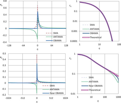
The method is illustrated in Fig. 2 using two example processes. The first is the Markov process, whose basic properties are:

(39) $c\left(h\right)=\lambda {\mathrm{e}}^{-\left|h\right|/\alpha },\gamma \left(k\right)=\frac{2\lambda }{k/\alpha }\left(1-\frac{1-{\mathrm{e}}^{-k/\alpha }}{k/\alpha }\right),\text{break}{c}_{\eta }=\frac{\lambda {\left(1-e^{-D/\alpha }\right)}^2}{{\left(D/\alpha \right)}^2}{e}^{-\left(\eta -1\right)D/\alpha },\eta \ge 1$(39)

The second is the FHK model defined in Eq. (13), which gives its climacogram, whilst all its other properties are evaluated through Eqs. (21)-(22). Figure 2 shows three special cases, SMA (Eq. (32)), ANTAMA (Eq. (33)) and OBAMA for the two processes. For the OBAMA case and the Markov process the exact Eq. (38) is used while for the FHK-C process the coefficients $a_{\eta }$ are determined from the approximate equation (B2) in Appendix B (with optimized coefficients of the equation). Some slight (rather invisible) deviations from zero are present in the left-bottom panel, which at a later step will be set to zero and the small resulting effect will be further handled as a truncation error (in the manner described by Koutsoyiannis 2016) to obtain an exact OBAMA scheme.

All in all, this simple method of the AMA scheme renders ARMA models unnecessary, particularly because of the generic, analytical and fast solution it offers. Here it is important to stress that, while optimization of coefficients involved in the function $\theta \left(\omega \right)$ could sometimes be necessary as discussed above and specified in Appendix B, it is not necessary in general. Any odd real function $\theta \left(\omega \right)$, chosen arbitrarily, will give $a_{\eta }$ that will satisfy Eq. (25) (apart from a truncation error) and thus can directly be used in generation. Even if the sequence of $\theta \left({\omega }_j\right)$ is constructed at random (e.g. as a sequence of random numbers in the interval [0,1/4]), again Eq. (25) will be satisfied and the resulting $a_{\eta }$ can directly be used in generation. (This case is also implemented on the spreadsheet provided as supplementary information).

6 Additional methodological issues

6.1 The AMA scheme in forecast mode

It is generally believed that AR models are better suited to forecast as they depend on past variables rather than on multiple innovation variables. According to this logic, among the MA models, only backward schemes would be suitable for forecast, while the generic AMA scheme (including the special case of SMA) would not, because it involves convolutions for both positive and negative lags η. Such beliefs are not quite correct though. Arguably, the forecast problem could be regarded as totally independent of the stochastic model per se, while forecasts can be obtained from any stochastic model, not only from a backward one. Had this not been the case, we would be in a deadlock in providing forecasts even with AR models. To see this, we may consider the case of an AR(p) scheme used to approximate a process with LRD. Because of LRD, the value of p will be large, typically larger than the number (n) of known past observations ($p>n)$. Therefore, the mathematical expression of the AR(p) as a weighted sum of past values could not be applied for forecast because some of the required past values would not be known.

Koutsoyiannis (2000) formulated a simple and general solution of the forecast problem, which can be applied for any type of linear model and hence for AMA. This calculates the prediction ${\widehat{\underset{\_}{x}}}_{\tau }$ for any future time τ combining, on the one hand, any simulation ${\underset{\_}{x}}_{\tau }$ independent of the observations, and, on the other hand, the observations $\widehat{\underset{\_}{z}}$, through the equations:

(40) ${\widehat{\underset{\_}{x}}}_{\tau }={\underset{\_}{x}}_{\tau }+c_{\tau }^{\text{T}}{C}^{-1}\left(\widehat{\underset{\_}{z}}-\underset{\_}{z}\right),\text{var}\left[{\widehat{\underset{\_}{x}}}_{\tau }|\widehat{\underset{\_}{z}}\right]={\gamma }_1-c_{\tau }^{\text{T}}{C}^{-1}{c}_{\tau }$(40)

where $\underset{\_}{\hat{z}}:={\left[{\underset{\_}{\hat{x}}}_0,{\underset{\_}{\hat{x}}}_{-1},\dots ,{\underset{\_}{\hat{x}}}_{-n}\right]}^{\mathrm{T}}$ is a vector containing the observations at the present (${\underset{\_}{\hat{x}}}_0$) and past times (${\underset{\_}{\hat{x}}}_{-1},\dots ,{\underset{\_}{\hat{x}}}_{-n}$), and $\underset{\_}{z}:={\left[{\underset{\_}{x}}_0,{\underset{\_}{x}}_{-1},\dots ,{\underset{\_}{x}}_{-n}\right]}^{\text{T}}$ is a vector containing the independently simulated items of the stochastic process at the present and past, whilst $c_{\tau }:=\text{cov}\left[{\underset{\_}{x}}_{\tau },\underset{\_}{z}\right]$ and $C:=cov\left[\underset{\_}{z},\underset{\_}{z}\right]$ are a vector and a matrix of covariances, respectively, with items determined from the chosen stochastic model (again, not estimated from the data).

6.2 Time asymmetry

Time irreversibility can very easily be handled within the AMA framework. Assuming that the white noise ${\underset{\_}{v}}_{\tau }$ (in discrete-time τ) has variance 1 and coefficient of skewness $C_{\mathrm{S}}^{\left(v\right)}$, we will have:

(41) $\begin{array}{rl}& \mathrm{v}\mathrm{a}\mathrm{r}\left[{\underset{\_}{x}}_{\tau }\right]=\sum _{j=-J}^J{a}_j^2,{\mu }_3\left[{\underset{\_}{x}}_{\tau }\right]=\sum _{j=-J}^J{a}_j^3{C}_{\mathrm{S}}^{\left(v\right)},\\ & C_{\mathrm{S}}:=\frac{{\mu }_3\left[{\hspace{0.17em}}_{\tau }\right]}{{\left(\mathrm{v}\mathrm{a}\mathrm{r}\left[{\underset{\_}{x}}_{\tau }\right]\right)}^{3/2}}=\frac{{\sum }_{j=-J}^J{a}_j^3}{{\left({\sum }_{j=-J}^J{a}_j^2\right)}^{3/2}}{C}_{\mathrm{S}}^{\left(v\right)}\end{array}$(41)

where ${\mu }_3\left[{\underset{\_}{x}}_{\tau }\right]$ and $C_{\mathrm{S}}$ are the third moment and the coefficient of skewness of process ${\underset{\_}{x}}_{\tau }$, respectively.

Time asymmetry is quantified through the skewness of the differenced process ${\underset{\_}{\tilde{x}}}_{\tau }$, according to Eq. (4), which by virtue of (24) is written as:

(42) ${\underset{\_}{\tilde{x}}}_{\tau }:={\underset{\_}{x}}_{\tau }-{\underset{\_}{x}}_{\tau -1}={\displaystyle \sum _{j=-J}^J\left(a_j-a_{j-1}\right)}{\underset{\_}{v}}_{\tau -j}$(42)

with $a_{-J-1}=0$. Thus, its skewness will be:

(43) ${\tilde{C}}_{\mathrm{S}}:=\frac{{\mu }_3\left[{\underset{\_}{\tilde{x}}}_{\tau }\right]}{{\left(var\left[{\underset{\_}{\tilde{x}}}_{\tau }\right]\right)}^{3/2}}=\frac{{\sum }_{j=-J}^J{\left(a_j-a_{j-1}\right)}^3}{{\left({\sum }_{j=-J}^J{\left(a_j-a_{j-1}\right)}^2\right)}^{3/2}}{C}_{\mathrm{S}}^{\left(v\right)}$(43)

The ratio:

(44) $\frac{{\tilde{C}}_{\mathrm{S}}}{C_{\mathrm{S}}}=\frac{{\sum }_{j=-J}^J{\left(a_j-a_{j-1}\right)}^3}{{\left({\sum }_{j=-J}^J{\left(a_j-a_{j-1}\right)}^2\right)}^{3/2}}\frac{{\left({\sum }_{j=-J}^J{a}_j^2\right)}^{3/2}}{{\sum }_{j=-J}^J{a}_j^3}$(44)

is independent of $C_{\mathrm{S}}^{\left(v\right)}$ and primarily depends on $\theta \left(\omega \right)$, which determines the sequence of $a_{\eta }$. The case $\theta \left(\omega \right)=0$, i.e. the SMA, results in complete time symmetry. However, a constant ${\theta }_0\ne 0$ (appropriately chosen) can make the ratio ${\tilde{C}}_{\mathrm{S}}/C_{\mathrm{S}}$ as high as we wish, thus enabling the preservation of time asymmetry.

The above results make it clear that without skewness in the original process ${\underset{\_}{x}}_{\tau }$ (e.g. in the case of Gaussian processes), there cannot be time asymmetry, a result that is consistent with Weiss’s (1975).

7 Application

Here we repeat the application in Koutsoyiannis (2019b) for the streamflow time series but using the new analytical framework. The data are from the database of the US Geological Survey⁶ for the site USGS 01603000 North Branch Potomac River Near Cumberland, Maryland (39°37ʹ18.5”N, 78°46ʹ24.3”W, catchment area: 2271 km²). They cover the period 2013-10-01 to 2018-08-31 for a time step of 15 min, which was aggregated to hourly, while discharge was converted from cubic feet per second to m³/s. Missing values (4% for a total of 172 416 values) were left unfilled. Seasonality is not negligible and was treated by standardizing the values of each month by an appropriate coefficient (see Koutsoyiannis 2019b). We note here that this standardization is just a rough modelling approximation, adequate for our aim to investigate time irreversibility, while an approach for operational use would require the construction of a cyclostationary model.

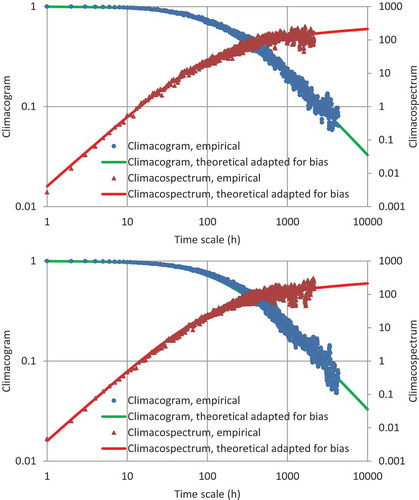
The process ${\underset{\_}{x}}_{\tau }$ is modelled as an FHK-C process; the fitting is impressively good and the parameters are M = 0.56 (indicating a slightly smooth process), H = 0.6 (a persistent process), α = 160 h and λ = γ(0) = 1.01 (for the standardized process). The fitting is shown in Fig. 3 in terms of the climacogram, which is good for visualizing the behaviour at large time scales, and the climacospectrum, which provides a better visualization for small time scales.

Figure 3. Comparison with the FHK-C model of the climacogram and climacospectrum of the original series, after standardization for dealing with seasonality (top); and of the generated series (bottom).

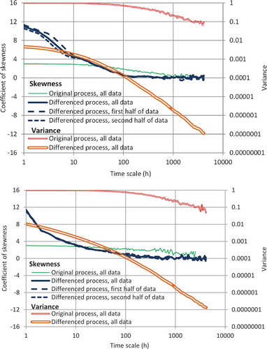
Additional parameters, quantifying the state and time asymmetry, are the skewness coefficients of the original and differenced process. The analysis in Koutsoyiannis (2019b) suggested prominent time irreversibility at time scales from 1 h to about 4 d. This is quantified by a skewness coefficient of the differenced process, which is much higher than the skewness of the original process ${\underset{\_}{x}}_{\tau }$ (10.99 for ${\underset{\_}{\tilde{x}}}_{\tau }$ and 2.98 for ${\underset{\_}{x}}_{\tau }$ at the hourly scale, a ratio ${\tilde{C}}_{\mathrm{S}}/C_{\mathrm{S}}=3.69$).

For the application, we use the proposed method with constant ${\theta }_0$ and with J = 1024. We note that the SMA case results in zero skewness of the differenced process (time symmetry) while in the ANTAMA case the skewness tends to infinity, which indicates that the method does not have any upper limit of time irreversibility that it can handle. Choosing ${\theta }_0=0.0638$, we make the ratio of the skewness of ${\underset{\_}{\tilde{x}}}_{\tau }$ and ${\underset{\_}{x}}_{\tau }$ equal to 3.69, as required. The coefficients $a_{\eta }$ determined by direct application of the method are shown in Fig. 4, along with the climacogram and the autocorrelation function of the original process.

Figure 4. Climacogram, autocorrelation and coefficients a_η determined by the proposed method.

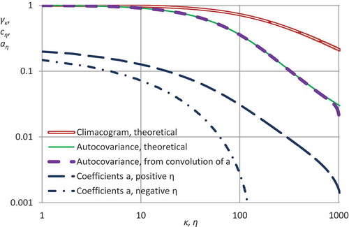
Figure 5. Generated discharge time series (top) (time references are arbitrary) and close-up for a six-month period containing the highest generated discharges (bottom). Plots refer to the “naturalized” (back-transformed) series.

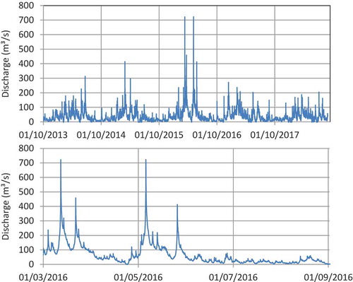
Figure 6. Climacograms and skewness coefficients of the original and differenced time series for: the real-world data (top) and the generated data (bottom). Plots refer to the standardized series.

For the generation of $v_i$ we use lognormal white noise with skewness determined so that the skewness of the original process be 2.98 as required. A time series with length equal to that of the real-world data was derived for the process ${\underset{\_}{x}}_{\tau }$ using Eq. (24) and was then “naturalized” by applying the inverse seasonal transformation. Plots for the generated time series are shown in Fig. 5, where in the close-up (lower panel) the irreversibility is evident, with steeper rising branches and milder falling ones. Comparisons of the generated time series with the model, as well as with the real-world data, in terms of climacogram and climacospectrum, are shown in Fig. 3. Comparisons of the characteristics related to state and time asymmetry are shown in Fig. 6. It is observed that the generated time series is consistent with the model and the original data in terms of all important statistics, marginal and joint, as well as related to time irreversibility. One slight discrepancy is that the curve related to time asymmetry in Fig. 6, while it captures the skewness of the real-world differenced data for the hourly scale, has a steeper slope for intermediate time scales; however, controlling this slope was not in the scope of this study. All in all, the method seems successful in simulation of streamflow time series even at fine time scales.

8 Conclusions

The main contribution of this article is the introduction of an equation that determines analytically the weights $a_{\eta }$ of an asymmetric moving average (AMA) scheme, which can be used in any problem of stochastic simulation of time-irreversible processes. This equation is rewritten here as:

(45) $a_{\eta }=\underset{-1/2}{\overset{1/2}{\int }}\sqrt{2}{\mathrm{e}}^{2\pi \mathrm{i}\left(\theta \left(\omega \right)-\eta \omega \right)}\sqrt{s_{\mathrm{d}}\left(\omega \right)}\mathrm{d}\omega$(45)

where $s_{\mathrm{d}}\left(\omega \right)$ is the power spectrum of the discrete-time representation of the process of interest and $\theta \left(\omega \right)$ is any arbitrary odd real function. The same equation can also be used for time-reversible processes, even though in this case it suffices to use the simpler symmetric (SMA) scheme, which can be obtained as a special case of the AMA for $\theta \left(\omega \right)=0$. In this case, the equation simplifies to:

(46) $a_{\eta }^{\mathrm{S}}=\underset{0}{\overset{1/2}{\int }}\sqrt{2}cos\left(2\pi \eta \omega \right)\sqrt{s_{\mathrm{d}}\left(\omega \right)}\mathrm{d}\omega$(46)

A simple expression can also be obtained for any case where $\theta \left(\omega \right)$ is a constant θ₀ multiplied by the sign of ω. Assuming that an adequately large number of weights is used (so that the quantity ${\delta }_0$ be negligible) this expression becomes:

(47) $a_{\eta }=a_{\eta }^{\mathrm{S}}cos\left(2\pi {\theta }_0\right)+a_{\eta }^{\mathrm{A}}sin\left(2\pi {\theta }_0\right)$(47)

where

(48) $a_{\eta }^{\mathrm{A}}=\frac{1}{2}\underset{0}{\overset{1/2}{\int }}\sqrt{2}sin\left(2\pi \eta \omega \right)\sqrt{s_{\mathrm{d}}\left(\omega \right)}\mathrm{d}\omega$(48)

is the antisymmetric solution (ANTAMA) of the equation.

The numerical evaluation of these weights is very easy and fast, as it only needs application of FFT, while the generation of the processes of interest is even easier; both are illustrated in a spreadsheet provided as supplementary information. The applicability of the method has no restrictions and no iterations are needed. Once the process dependence is known through any second-order tool (climacogram, autocovariance, power spectrum, etc.) and the properties related to time reversibility or irreversibility are specified, the method can be readily applied for stochastic generation.

The extended historical review presented in this article reveals that the proposed method is against the current of simulation approaches that were developed since the 1950s. Specifically, the approach proposed (a) uses a purely moving-average scheme, without any autoregressive term, (b) involves innovation terms and weights that extend to both directions of time, and (c) does not link the generation scheme with the observations – rather, the observations are used in the model fitting phase, which is independent of the simulation. Because of the moving-average scheme we are able to easily handle and preserve moments higher than second. Because of the involvement of terms in both directions of time in an asymmetric mode, we can easily reproduce time irreversibility in a controlled manner. And because of the separation of model fitting from the calculation of the weights of the linear model, we are able to handle any type of dependence in time for whatever range (short or long) and fractality (smooth or rough). For the same reason, we are able to make the model as parsimonious as we wish (and as the data allow) without being trapped to involve many parameters in order to preserve, for example, autocovariances of large lags.

The entire framework is so simple and powerful that one can hardly believe that it is presented for the first time. Perhaps it is a reinvention of something already known. Whether it has been invented or not in the past, the fact is that it is not well known (and certainly not known to the author); otherwise, the ARMA models and their variants would not be so popular. Hopefully, this article could contribute to give ARMA-type models a position in the history of stochastics.

Acknowledgements

I thank the eponymous reviewers William Farmer and Alberto Montanari for their extraordinarily constructive comments which encouraged me to broaden, completely restructure and, eventually, substantially improve the initial manuscript. During the preparation of the second version of the manuscript, I had the pleasure to present its content in a seminar in the Sapienza University of Rome as well as in the First Workshop on Control Methods for Water Resource Systems in Delft. I wish to express my gratitude to Francesco Napolitano for inviting and organizing my visit in Rome during September 2019, and Alla Kolechkina and Ronald van Nooyen for the invitation in the Workshop in Delft.

Disclosure statement

No potential conflict of interest was reported by the author.

Supplementary material

Supplemental data for this article can be accessed here.

Additional information

Funding

No funding was provided for this research.

Notes

¹ Boltzmann coined the terms ergode and isodic, both of which are etymologized from Greek words but which ones exactly is uncertain. Most probably, ergodic comes from the Greek ἔργον (ergon = work) and ὁδός (hodos = pathway). According to another interpretation, the second noun is είδος (eidos = form, kind, nature), or the whole word is a transliteration of the Greek adjective ἐργώδης (ergodes = laborious, troublesome; see Mathieu 1988).

² The Greek adjective “stochastic[os/e]” was used by Greek philosophers, including Plato and Aristotle, and was transplanted to the international scientific vocabulary by Jacob Bernoulli (evidently aware of the Greek literature and in particular of Plato’s texts) in his famous book Ars Conjectandi (written in Latin in 1684–89 but published after his death, in 1713). The term was revived by Bortkiewicz (1917; Russian economist and statistician of Polish ancestry) and also by Slutsky (1925, 1928a, 1928b, 1929; Ukrainian/Russian/Soviet mathematical statistician and economist). It appears that the prevalence in USSR of the more sophisticated term “stochastic” (over the rather equivalent term “random”) must have been related to political and ideological reasons (incongruence of randomness with the dialectic materialism: models beyond strict deterministic were considered with a priori suspicion; see Mazliak 2018).

³ LeClerc’s Monte Carlo method to calculate π became popular among scientists and his experiment was later repeated by many. There are many other Monte Carlo algorithms to estimate π. However, these are good only for fun, as much faster and much more accurate deterministic algorithms exist to calculate π. Reitwiesner (1950) calculated by a deterministic algorithm, running on the ENIAC computer, the first 2035 decimal digits of π. Metropolis et al. (1950) examined their randomness, an exercise made thereafter many times showing that the digits of π have no apparent pattern and pass tests for statistical randomness. Dodge (1996) promoted an idea opposite to LeClerc’s: that the digits of π form a “Natural Random Number Generator”. Since January 2019, 31.4 trillion digits of π are known (found by the Chudnovsky algorithm); this information, equivalent to ~100 million books of 1000 pages each (note for comparison that the British Library has 25 million books), can serve as a basis for any simulation experiment. However, simple random generators are more economic and convenient.

⁴ Notably, Ulam conceived the method while playing solitaires during convalescing from an illness, in his attempt to estimate the probabilities of success of the plays. As Ulam describes the story in some remarks later published by Eckhardt (1989), “After spending a lot of time to estimate them by pure combinatorial calculations, I wondered whether a more practical method than ‘abstract thinking’ might not be to lay it out say one hundred times and simply observe and count the number of successful plays.”

⁵ The term climacogram, from the Greek κλιμακόγραμμα, deriving from κλίμαξ (climax = scale, as well as ladder; pl. κλίμακες) and γράμμα (gramma = written, drawn), was coined by Koutsoyiannis (2010) and could be translated in English as scale(o)gram, but the latter term is used for another concept. Climacogram should not be confused to climatogram which has another meaning related to the climatic regime of temperature and precipitation at a site or area. The latter term, deriving from the noun κλίμα (clima, originally meaning slope; pl. κλίματα), was first used in the Hellenistic period by the astronomer Hipparchus to describe climate (in relationship to the slope of the sun’s rays) and is different from the other derivative noun κλίμαξ. Interestingly though, both κλίμαξ and κλίμα are eventually etymologized from the same verb κλίνειν (klinein = to slope).

⁶ https://nwis.waterdata.usgs.gov/md/nwis/uv/?site_no = 01603000&agency_cd = USGS, retrieved: 2018-09-16.

Appendix A

Proof of the basic properties of the AMA solution

To show point (a) below Eq. (27), we observe that the sequence of $a_{\eta }$ is the finite Fourier transform of:

(A1) $A\left(\omega \right):={\mathrm{e}}^{2\pi \mathrm{i}\theta \left(\omega \right)}{A}^{\mathrm{R}}\left(\omega \right)=\left(cos\left(2\pi \theta \left(\omega \right)\right)+\mathrm{i}sin\left(2\pi \theta \left(\omega \right)\right)\right)A^{\mathrm{R}}\left(\omega \right)$(A1)

We recall that the power spectrum $s\left(\omega \right)$ is an even function, and so are $s_{\mathrm{d}}\left(\omega \right)$ and $A^{\mathrm{R}}\left(\omega \right)$. Besides $cos\left(2\pi \theta \left(\omega \right)\right)$ is also even, while $sin\left(2\pi \theta \left(\omega \right)\right)$ is odd, given that $\theta \left(\omega \right)$ is odd. Consequently, $A\left(\omega \right)$ has even real part and odd imaginary part. Hence, its Fourier transform is real (Bracewell 2000, p. 13), which proves that $a_{\eta }$ is real. It can also be written as a real expression:

(A2) $a_{\eta }=2\underset{0}{\overset{1/2}{\int }}cos\left(2\pi \left(\theta \left(\omega \right)-\eta \omega \right)\right)A^{\mathrm{R}}\left(\omega \right)\mathrm{d}\omega$(A2)

To show point (b), we observe that $A\left(\omega \right)$ is the inverse finite Fourier transform of $a_{\eta }$, i.e.

$A\left(\omega \right)=2\sum _{l=-\mathrm{\infty }}^{\mathrm{\infty }}{a}_l{\mathrm{e}}^{2\pi \mathrm{i}l\omega }$

Besides, the inverse finite Fourier transform of the quantity $c_{\eta }^{\prime }:=\sum _{l=-\mathrm{\infty }}^{\mathrm{\infty }}{a}_l{a}_{\eta +l}$ is

(A3) $\begin{array}{rl}& B\left(\omega \right)=2\sum _{\eta =-\mathrm{\infty }}^{\mathrm{\infty }}{c}_{\eta }^{\prime }{\mathrm{e}}^{2\pi \mathrm{i}\eta \omega }=2\sum _{\eta =-\mathrm{\infty }}^{\mathrm{\infty }}\sum _{l=-\mathrm{\infty }}^{\mathrm{\infty }}{a}_l{a}_{\eta +l}{\mathrm{e}}^{2\pi \mathrm{i}\eta \omega }\\ & =2\sum _{l=-\mathrm{\infty }}^{\mathrm{\infty }}{a}_l\sum _{\eta =-\mathrm{\infty }}^{\mathrm{\infty }}{a}_{\eta +l}{\mathrm{e}}^{2\pi \mathrm{i}\eta \omega }\\ & =2\sum _{l=-\mathrm{\infty }}^{\mathrm{\infty }}{a}_l\sum _{j=-\mathrm{\infty }}^{\mathrm{\infty }}{a}_j{\mathrm{e}}^{2\pi \mathrm{i}\left(j-l\right)\omega }=2\sum _{l=-\mathrm{\infty }}^{\mathrm{\infty }}{a}_l{\mathrm{e}}^{-2\pi \mathrm{i}l\omega }\sum _{j=-\mathrm{\infty }}^{\mathrm{\infty }}{a}_j{\mathrm{e}}^{2\pi \mathrm{i}j\omega }\\ & =\frac{A{\left(\omega \right)}^{\ast }A\left(\omega \right)}{2}\end{array}$(A3)

where $A{\left(\omega \right)}^{\ast }$ is the conjugate of $A\left(\omega \right)$, equal to ${\mathrm{e}}^{-2\pi \mathrm{i}\theta \left(\omega \right)}{A}^{\mathrm{R}}\left(\omega \right)$. Consequently,

(A4) $B\left(\omega \right)=\frac{A{\left(\omega \right)}^{\ast }A\left(\omega \right)}{2}=\frac{{\mathrm{e}}^{-2\pi \mathrm{i}\theta \left(\omega \right)}{A}^{\mathrm{R}}\left(\omega \right){\mathrm{e}}^{2\pi \mathrm{i}\theta \left(\omega \right)}{A}^{\mathrm{R}}\left(\omega \right)}{2}=\frac{{\left(A^{\mathrm{R}}\left(\omega \right)\right)}^2}{2}=s_{\mathrm{d}}\left(\omega \right)$(A4)

where we have utilized the definition of $A^{\mathrm{R}}\left(\omega \right)$ in (27). Hence, the Fourier transform of $c_{\eta }^{\prime }$ equals the power spectrum, which means that $c_{\eta }^{\prime }$ is identical to the autocovariance function $c_{\eta }$.

Now, coming to point (c), the calculation of the sequence of coefficients $a_{\eta }$, and hence the generation of the required time series, we first note that, unlike in the above theoretical derivations, summation is in practice made for a finite number of terms, i.e. for $\eta =-J,\dots ,0,\dots ,J$, where J if finite. The coefficients $a_{\eta }$ will decrease with increasing η and will be negligible beyond an appropriately chosen, adequately large, J. Possible truncation errors can be handled as described by Koutsoyiannis (2016 – even though that solution was for the SMA scheme). For the numerical part, since we know the frequency functions $A^{\mathrm{R}}\left(\omega \right)$ (from the power spectrum) and $\theta \left(\omega \right)$ (appropriately or even arbitrarily or randomly chosen), for an array of frequencies ${\omega }_j$, we are able to write Eqs. (30)–(31) and complete the algorithm described in steps (i)-(iv) in Sec. 5.

Appendix B

The OBAMA scheme and other cases requiring optimization

If the process exhibits LRD and for some reason an OBAMA scheme is desired, one option would be to generalize Eq. (38) to the form:

(B1) $\theta \left(\omega \right)={\theta }_0+\frac{1}{2\pi }{cos}^{-1}\left({\left(\frac{1}{C_1\sqrt{s_{\mathrm{d}}\left(\omega \right)}}+\frac{\sqrt{s_{\mathrm{d}}\left(\omega \right)}}{C_2}\right)}^{C_0}\right),\omega >0$(B1)

where ${\theta }_0,C_0,C_1,C_2,$are coefficients to be optimized numerically, so that the deviation from zero of all $\eta <0$ (quantified e.g. by the mean square error) be minimal. Continuity at 0 of $\theta \left(\omega \right)$ is not necessary, but if required it can be achieved setting $\theta \left(0\right)=0$.

A second option, which was found quite satisfactory in numerical explorations, is to define $\theta \left(\omega \right)$ as the smooth minimum of two rational functions of frequency, ${\theta }_i\left(\omega \right),i=1,2,$ with first degree polynomials, i.e.:

(B2) $\theta \left(\omega \right)=\frac{1}{\zeta }ln\left(e^{\zeta {\theta }_1\left(\omega \right)}+e^{\zeta {\theta }_2\left(1/2-\omega \right)}\right),{\theta }_i\left(\omega \right):=\frac{C_{1,i}\omega }{C_{2,i}+\omega }+C_{0,i}$(B2)

where $C_{ji};i=1,2;j=0,1,2$ are coefficients with values to be optimized and $\zeta$ a big negative number, say, $\zeta =-10$. Optimizing each $\theta \left({\omega }_j\right)$, without using parametric relationships, is another option but in the LRD case the frequencies of interest ${\omega }_j$ will be numerous and, therefore, an expression such as (B1) or (B2), whose coefficients are optimized, may be an advantage.

We can use the same expressions for other tasks. For example, if for some reason we need an ordinary-backward scheme of ARMA type, again the framework provided can directly convert itself into an ARMA scheme. Thus, to convert AMA to an ARMA$\left(1,q\right)$ model, for which $a_{\eta }=0$ for $\eta <0$ and $a_{\eta }=\beta a_{\eta -1}={\beta }^{\eta -q}{a}_q$ for $\eta >q$ and for some appropriate β, we can form the objective function (representing the cumulative departure of the achieved sequence of coefficients from those of an ARMA$\left(1,q\right)$ model):

(B3) $e\left(a_0,\dots ,a_q;\beta \right):=\sum _{\eta =-J}^0{a}_{\eta }^2+\sum _{\eta =q}^J{\left(a_{\eta }-{\beta }^{\eta -q}{a}_q\right)}^2$(B3)

minimize it finding the vector of coefficients $\left(a_0,\dots ,a_q;\beta \right)$, and reformulate the generating Eq. (24) as:

(B4) ${\underset{\_}{x}}_{\tau }=\beta {\underset{\_}{x}}_{\tau -1}+{\displaystyle \sum }_{\eta =0}^q{a}_{\eta }{\underset{\_}{v}}_{\tau -\eta }$(B4)

so that a limited number of previous noise variables ${\underset{\_}{v}}_{\tau -\eta }$ and the latest process variable ${\underset{\_}{x}}_{\tau -1}$ are only needed. This case is also implemented in the spreadsheet provided as supplementary information. The same spreadsheet file contains also other cases, such as the conversion into an AR(q) model or to the sum of three AR(1) models, where the algorithms used are hopefully self-explanatory.

References

- Bailey, A.L., 1929. A summary of advanced statistical methods. US Statistical Bureau. https://babel.hathitrust.org/cgi/pt?id=mdp.39015067991326&view=1up&seq=7.
- Barnes, F.B., 1954. Storage required for a city water supply. The Institution of Engineers, Australia, 26, 198–203.
- Barnett, V., 2006. Chancing an interpretation: Slutsky’s random cycles revisited. The European Journal of the History of Economic Thought, 13 (3), 411–432. doi:10.1080/09672560600875596
- Beard, L.R., 1965. Use of interrelated records to simulate streamflow. Proceedings ASCE, Journal of the Hydraulics Division, 91 (HY5), 13–22.
- Birkhoff, G.D., 1931. Proof of the ergodic theorem. Proceedings of the National Academy of Sciences, 17, 656–660. doi:10.1073/pnas.17.2.656
- Boltzmann, L., 1877. Über die Beziehung zwischen dem zweiten Hauptsatze der mechanischen Wärmetheorie und der Wahrscheinlichkeitsrechnung respektive den Sätzen über das Wärmegleichgewicht. Wiener Ber, 76. 373–435. (in German).
- Boltzmann, L., 1884/85. Über die Eigenschaften monocyklischer und anderer damit verwandter Systeme. Crelles Journal, 98, 68–94.
- Bortkiewicz, L., 1917. Die iterationen — Ein beitrag zur wahrscheinlichkeitstheorie. Berlin: Springer.
- Box, G.E. and Jenkins, G.M., 1970. Time series models for forecasting and control. San Francisco, USA: Holden Day.
- Bracewell, R.N., 2000. The fourier transform and its applications. 3rd Ed. Boston, MA: McGraw-Hill.
- Chow, V.T., 1969. Stochastic analysis of hydrologic systems. Final Report. Urbana, IL: University of Illinois. https://www.ideals.illinois.edu/bitstream/handle/2142/90345/Chow_1969.pdf?sequence=2.
- Chow, V.T. and Kareliotis, S.J., 1970. Analysis of stochastic hydrologic systems. Water Resources Research, 6 (6), 1569–1582. doi:10.1029/WR006i006p01569
- Dimitriadis, P. and Koutsoyiannis, D., 2015. Climacogram versus autocovariance and power spectrum in stochastic modelling for Markovian and Hurst–Kolmogorov processes. Stochastic Environmental Research & Risk Assessment, 29 (6), 1649–1669. doi:10.1007/s00477-015-1023-7
- Dimitriadis, P. and Koutsoyiannis, D., 2018. Stochastic synthesis approximating any process dependence and distribution. Stochastic Environmental Research & Risk Assessment, 32 (6), 1493–1515. doi:10.1007/s00477-018-1540-2
- Dodge, Y., 1996. A natural random number generator. International Statistical Review, 64 (3), 329–344. doi:10.2307/1403789
- Eckhardt, R., 1989. Stan Ulam, John von Neumann and the Monte Carlo method. In: N.G. Cooper, ed. From cardinals to chaos. NY: Cambridge University, 131–136.
- Galton, F., 1890. Dice for statistical experiments. Nature, 42, 13–14. doi:10.1038/042013a0
- Gauch, H.G., Jr., 2003. Scientific method in practice. Cambridge, UK: Cambridge University Press.
- Hamed, K.H., 2008. Trend detection in hydrologic data: the Mann–Kendall trend test under the scaling hypothesis. Journal of Hydrology, 349 (3–4), 350–363. doi:10.1016/j.jhydrol.2007.11.009
- Hazen, A., 1914. Storage to be provided in impounding reservoirs for municipal water supply. Transactions of the American Society of Civil Engineers, 77, 1539–1640.
- Hosking, J.R.M., 1981. Fractional differencing. Biometrika, 68 (1), 165–176. doi:10.1093/biomet/68.1.165
- Hurst, H.E., 1951. Long term storage capacities of reservoirs. Transactions of the American Society of Civil Engineers, 116, 776–808.
- Kendall, M.G., 1938. A new measure of rank correlation. Biometrika, 30 (1/2), 81–93. doi:10.1093/biomet/30.1-2.81
- Khintchine, A., 1933. Zu Birkhoffs Lösung des Ergodenproblems. Mathematische Annalen, 107, 485–488. doi:10.1007/BF01448905
- Khintchine, A., 1934. Korrelationstheorie der stationären stochastischen Prozesse. Mathematische Annalen, 109 (1), 604–615. doi:10.1007/BF01449156
- Klemes, V., 1987. One hundred years of applied storage reservoir theory. Water Resources Management, 1 (3), 159–175. doi:10.1007/BF00429941
- Kolmogorov, A.N., 1931. Uber die analytischen Methoden in der Wahrscheinlichkcitsrechnung. Mathematische Annalen, 104, 415–458. (English edition: Kolmogorov, A.N., 1992. On analytical methods in probability theory. Selected Works of A. N. Kolmogorov - Volume 2, Probability Theory and Mathematical Statistics, A. N. Shiryayev, ed., Kluwer, Dordrecht, The Netherlands, pp. 62-108). doi:10.1007/BF01457949
- Kolmogorov, A.N., 1933. Grundbegriffe der Wahrscheinlichkeitsrechnung (Ergebnisse der Mathematik und Ihrer Grenzgebiete). Berlin: Springer. (2nd English Edition: Foundations of the Theory of Probability, 84 pp. Chelsea Publishing Company, New York, 1956).
- Kolmogorov, A.N., 1937. Ein vereinfachter Beweis der Birkhoff-Khintchineschen Ergodensatzes. Matematicheskii Sbornik, 2, 367–368.
- Kolmogorov, A.N., 1938. A simplified proof of the Birkhoff-Khinchin ergodic theorem. Uspekhi Matematicheskikh Nauk, 5. 52–56. (English edition: Kolmogorov, A.N., 1991, Selected Works of A. N. Kolmogorov - Volume 1, Mathematics and Mechanics, Tikhomirov, V. M. ed., Kluwer, Dordrecht, The Netherlands, pp. 271-276).
- Kolmogorov, A.N., 1940. Wienersche Spiralen und einige andere interessante Kurven im Hilbertschen Raum. Doklady Akademii Nauk SSSR, 26. 115–118. (English edition: Kolmogorov, A.N., 1991. Wiener spirals and some other interesting curves in a Hilbert space. Selected Works of A. N. Kolmogorov - Volume 1, Mathematics and Mechanics, Tikhomirov, V. M. ed., Kluwer, Dordrecht, The Netherlands, pp. 303-307).
- Kolmogorov, A.N., 1947. Statistical theory of oscillations with continuous spectrum. In: Collected papers on the 30th anniversary of the Great October Socialist Revolution. Vol. 1. Moscow-Leningrad: Akad. Nauk SSSR, 242–252. (English edition: Kolmogorov, A.N., 1992. Selected Works of A. N. Kolmogorov - Volume 2, Probability Theory and Mathematical Statistics, A. N. Shiryayev ed., Kluwer, Dordrecht, The Netherlands, pp. 321-330).
- Koutsoyiannis, D., 2000. A generalized mathematical framework for stochastic simulation and forecast of hydrologic time series. Water Resources Research, 36 (6), 1519–1533. doi:10.1029/2000WR900044
- Koutsoyiannis, D., 2010. A random walk on water. Hydrology and Earth System Sciences, 14, 585–601. doi:10.5194/hess-14-585-2010
- Koutsoyiannis, D., 2016. Generic and parsimonious stochastic modelling for hydrology and beyond. Hydrological Sciences Journal, 61 (2), 225–244. doi:10.1080/02626667.2015.1016950
- Koutsoyiannis, D., 2017. Entropy production in stochastics. Entropy, 19 (11), 581. doi:10.3390/e19110581
- Koutsoyiannis, D., 2019a. Knowable moments for high-order stochastic characterization and modelling of hydrological processes. Hydrological Sciences Journal, 64 (1), 19–33. doi:10.1080/02626667.2018.1556794
- Koutsoyiannis, D., 2019b. Time’s arrow in stochastic characterization and simulation of atmospheric and hydrological processes. Hydrological Sciences Journal, 64 (9), 1013–1037. doi:10.1080/02626667.2019.1600700
- Koutsoyiannis, D. and Montanari, A., 2015. Negligent killing of scientific concepts: the stationarity case. Hydrological Sciences Journal, 60 (7–8), 1174–1183. doi:10.1080/02626667.2014.959959
- Kyun, K. and Kim, K., 2006. Equilibrium business cycle theory in historical perspective. International Statistical Review.
- Lawrance, A.J., 1991. Directionality and reversibility in time series. International Statistical Review, 59 (1), 67–79. doi:10.2307/1403575
- Lombardo, F., et al., 2014. Just two moments! A cautionary note against use of high-order moments in multifractal models in hydrology. Hydrology and Earth System Sciences, 18, 243–255. doi:10.5194/hess-18-243-2014
- Mackey, M.C., 2003. Time’s arrow: the origins of thermodynamic behavior. Mineola, NY: Dover, 175.
- Mahalanobis, P.C., 1934. Tables of random samples from a normal population. Sankya, 1, 289–328.
- Mandelbrot, B.B. and Wallis, J.R., 1969. Computer experiments with fractional gaussian noises: part 1, averages and variances. Water Resources Research, 5, 228–241. doi:10.1029/WR005i001p00228
- Mann, H.B., 1945. Nonparametric tests against trend. Econometrica, 13 (3), 245–259. doi:10.2307/1907187
- Matalas, N.C., 1967. Mathematical assessment of synthetic hydrology. Water Resources Research, 3 (4), 937–945. doi:10.1029/WR003i004p00937
- Mathieu, M., 1988. On the origin of the notion ‘Ergodic Theory’. Expositiones Mathematicae, 6, 373–377.
- Mazliak, L., 2018. The beginnings of the Soviet encyclopedia. The utopia and misery of mathematics in the political turmoil of the 1920s. Centaurus, 60 (1–2), 25–51. doi:10.1111/cnt.2018.60.issue-1-2
- Metropolis, N., 1989. The beginning of the Monte Carlo method. In: N.G. Cooper, ed.. From cardinals to chaos. NY: Cambridge University, 125–130.
- Metropolis, N., Reitwiesner, G., and von Neumann, J., 1950. Statistical treatment of values of first 2,000 decimal digits of e and of π calculated on the ENIAC. Mathematical Tables and Other Aids to Computation, 4, 109–112. doi:10.2307/2002776
- Metropolis, N. and Ulam, S.M., 1949. The Monte Carlo method. Journal of the American Statistical Association, 44, 335–341. doi:10.1080/01621459.1949.10483310
- Montanari, A. and Koutsoyiannis, D., 2014. Modeling and mitigating natural hazards: stationarity is immortal! Water Resources Research, 50 (12), 9748–9756. doi:10.1002/2014WR016092
- Niederreiter, Η., 1992. Random number generation and quasi-Monte Carlo methods. Philadelphia: Society for Industrial and Applied Mathematics.
- O’Connell, P.E., et al., 2016. The scientific legacy of Harold Edwin Hurst (1880 – 1978). Hydrological Sciences Journal, 61 (9), 1571–1590. doi:10.1080/02626667.2015.1125998
- Papoulis, A., 1991. Probability, Random Variables and Stochastic Processes. 3rd Ed. New York: McGraw-Hill.
- Persons, W.M. 1919. Measuring and forecasting general business conditions. Harvard University & American Institute of Finance. https://babel.hathitrust.org/cgi/pt?id=hvd.32044018749697
- Reitwiesner, G., 1950. An ENIAC Determination of π and e to more than 2000 Decimal Places. Mathematical Tables and Other Aids to Computation, 4, 11–15. doi:10.2307/2002695
- Slutsky, E., 1927. Slozhenie sluchainykh prichin, kak istochnik tsiklicheskikh protsessov. Voprosy Kon”yunktury, 3. 34–64. [English edition: Slutsky, E., 1937. The summation of random causes as the source of cyclic processes. Econometrica: Journal of the Econometric Society, 105-146].
- Slutsky, E., 1928a. Sur ùn critérium de la convergence stochastique des ensembles des valeurs éventuelles). Comptes Rendus De l’Académie Des Sciences, 187, 370.
- Slutsky, E., 1925. Über stochastische Asymptoten und Grenzwerte. Metron, 5 (3), 3–89.
- Slutsky, E., 1928b. Sur les fonctions éventuelles continues, intégrables et dérivables dans le sens stochastiques. Comptes Rendus Des Séances De l’Académie Des Sciences, 187, 878.
- Slutsky, E., 1929. Quelques propositions sur les limites stochastiques éventuelles. Comptes Rendus Des Séances De l’Académie Des Sciences, 189, 384.
- Stigler, S.M., 2002. Statistics on the table: the history of statistical concepts and methods. Cambridge, MA: Harvard University Press.
- Sudler, C., 1927. Storage required for the regulation of streamflow. Transactions of the American Society of Civil Engineers, 91, 622–660.
- Thomas, H.A. and Fiering, M.B., 1962. Mathematical synthesis of streamflow sequences for the analysis of river basins by simulation. In: A. Maass, et al., eds.. Design of water resource systems. Cambridge, MA: Harvard University Press, 459–493.
- Tippett, L.H.C., 1927. Random sampling numbers. London: Cambridge University Press, Tracts for Computers No. XV.
- Tong, H. and Zhang, Z., 2005. On time-reversibility of multivariate linear processes. Statistica Sinica, 15 (2), 495–504.
- Walker, G., 1931. On periodicity in series of related terms. Proceedings of the Royal Society of London, Series A, 131, 518–532. doi:10.1098/rspa.1931.0069
- Weiss, G., 1975. Time-reversibility of linear stochastic processes. Journal of Applied Probability, 12 (4), 831–836. doi:10.2307/3212735
- Whittle, P., 1951. Hypothesis testing in times series analysis. PhD thesis, Almqvist & Wiksells, Uppsala.
- Whittle, P., 1952. Tests of fit in time series. Biometrika, 39 (3/4), 309–318. doi:10.1093/biomet/39.3-4.309
- Whittle, P., 1953. The analysis of multiple stationary time series. Journal of the Royal Statistical Society B, 15 (1), 125–139.
- Wold, H.O., 1938. A study in the analysis of stationary time-series. PhD thesis, Almquist and Wicksell, Uppsala.
- Wold, H.O., 1948. On prediction in stationary time series. The Annals of Mathematical Statistics, 19 (4), 558–567. doi:10.1214/aoms/1177730151
- Yule, G.U., 1927. On a method of investigating periodicities in disturbed series, with special reference to Wolfer’s sunspot numbers. Philosophical Transactions of the Royal Society of London A, 226, 267–298. doi:10.1098/rsta.1927.0007