Seasonal patterns of suspended sediment load and erosion-transport assessment in a Mediterranean basin

ABSTRACT

To assess seasonal patterns of suspended sediment load and its erosion–transport interactions, 17 years of river monitoring data from the Isser River Basin (northwest Algeria) were studied, considering continuous and event-scale approaches. The results show significant differences in sediment yield and transport processes between dry and wet periods. A rate of 8 t ha⁻¹ year⁻¹ was estimated from continuous analysis, with values of 4.3 and 13 t ha⁻¹ year⁻¹ for wet and dry periods, respectively. Estimates of soil delivery ratio pointed to higher values during dry periods and the dominance of hillslope erosion processes. At the event scale, the hysteresis loops confirmed these seasonal patterns in transport dynamics. The calibration of the MUSLE model highlighted the severity of rainfall during the dry period. These results emphasize the importance of seasonality in erosion and transport processes with special relevance in terms of climate change predictions.

KEYWORDS:

• suspended load
• sediment yield
• seasonality
• Modified Universal Soil Loss Equation (MUSLE)
• sediment delivery

Editor S. ArchfieldAssociate editor M. Hutchins

1 Introduction

Soil erosion and sedimentation are considered as one of the major threats affecting agriculture, water resource management and ecosystem services (Rodríguez et al. 2006, Yu 2012, Prosdocimi et al. 2016, Balla et al. 2017). According to Pimentel et al. (1995), more than 75 billion tons of arable land have been lost due to erosion processes worldwide. The cost associated with this loss in soil resources related to the edaphic layer is up to US$18 billion (Bernoux et al. 2006, Schwegler 2014). However, the urgent need to improve erosion management strategies collides with the lack of knowledge on erosion and transport processes. The scarce available data and the difficulty in estimating a global budget of sediment delivered remain important challenges (Walling et al. 2001, Chalov et al. 2017).

The first step in the fight against soil erosion and its effects downstream requires appropriate land-use planning at hillslopes and fluvial systems based on a thorough knowledge of both landscape degradation (Ferreira and Panagopoulos 2012, Perović et al. 2013) and transport process assessment (Millares and Moñino 2018a). Approaches based on the sediment budget concept represent a holistic view of erosive and sedimentary processes throughout a basin, and involve: (a) soil loss assessment, usually given by its specific sediment yield (SSY) in mass per surface and time units; (b) characterization of fluvial processes along the channel; and (c) estimation of the fraction of transported sediment that comes out at the basin outlet, or the sediment delivery ratio (SDR). This index and its assessment have been discussed in depth in previous works due to its great complexity and the related uncertainties (e.g. Walling 1999, Parsons et al. 2008).

The fractions belonging to fluvial and hillslope systems are very variable depending on geological settings, pluviometric regime, channel morphology, land use or climate conditions, as reported in the literature (e.g. Church and Slaymaker 1989, Walling and Webb 1996, Walling 1999, Buffington and Montgomery 2013). Furthermore, at the basin scale, the value of SSY has been generally associated with soil loss and the continuous suspended load contributions related to different controlling factors and forcing agents (Zabaleta et al. 2007, Faran Ali and de Boer 2008, Nadal‐Romero et al. 2013, Rainato et al. 2018, Millares et al. 2018b). However, interpreting the influence of erosion processes on sediment delivery and transport processes requires intensive monitoring and modelling tasks (Wasson 2002).

The temporal relationship between suspended sediment concentration (SSC) and water discharge (Q) provides an integrated analysis of time-varying sediment supply. This relationship depends on different factors, such as rainfall intensity, soil moisture, or the duration and flow responses (Seeger et al. 2004, Smith and Dragovich 2009). The hysteresis patterns or loops have been frequently used for understanding sediment transport processes by interpreting the spatial distribution of sediment sources, the dynamics of rain erosivity, or the differences in travel times between waves of water and sediment discharge (Gregory and Walling 1973, Williams 1989, Lenzi and Marchi 2000, Pietroń et al. 2015). They have been key in identifying seasonal patterns in erosive and transport dynamics in Mediterranean basins (Batalla and Sala 1994, Farguell and Sala 2006, Khanchoul et al. 2009, De Girolamo et al. 2015, Selmi and Khanchoul 2016).

Soil loss presents an important seasonal behaviour, greatly related to the intensity of precipitation events and vegetation cover, which impacts on sediment yield. This is especially relevant in Mediterranean environments, characterized by the strong variability of precipitation, intense rainfall events and alternations of severe drought cycles (Meddi et al. 2009, Tramblay et al. 2013, Zettam et al. 2017). In the Maghreb region, previous studies have highlighted the relationship between erosive dynamics and agricultural practices, rock erodibility and annual runoff (Probst and Suchet 1992).

Walling (1984) estimated rates of SSY between 10 and 50 t ha⁻¹ year⁻¹ in countries of this region. In Morocco, soil erosion threatens up to 12.5 × 10⁶ ha in crop and rangeland (Naimi et al. 2005), with specific degradation exceeding 20 t ha⁻¹ year⁻¹ (Ghanam 2003). Tunisia loses more than 15 000 ha of agricultural land each year due to erosion processes (Slim and Jeddi 2011), with the annual loss of its reservoir capacity being more than 0.5% (Saadaoui 1996).

In northern Algeria, soil erosion and sedimentation have led to important and catastrophic damage affecting several sectors of the country. These processes are responsible for decreasing water availability, complicate the management of protected areas (Bouchetata and Bouchetata 2006, Salhi et al. 2013) and affect agricultural production (Boughalem et al. 2014). Large rates of erosion, of between 23 and 72 t ha⁻¹ year⁻¹ in certain areas of Algeria, results in more than 50 hm³ of volume loss of reservoir capacity (Megnounif et al. 2003, Tachi et al. 2016, Remini and Bensafia 2016). Furthermore, these processes have greatly increased during the last decades from 20 hm³ of dam siltation in 1980 to 45 hm³ in 2000 (Serbah 2011, Tachi et al. 2016).

Assessing actual soil loss and erosion rates throughout field campaigns is usually expensive and time consuming (Barthes and Roose 2002). Furthermore, the great spatial and temporal variability of soil erosion, especially in Mediterranean environments, limits the extrapolations of on-site measurements (Millares and Moñino 2018a). In contrast, indirect approaches, such as empirical or parametric models, physically based hydrological modelling or remote sensing analysis provide valuable information on erosion rates and potential soil loss with reasonable associated costs (Boultif and Benmessaoud 2017, Sepuru and Dube 2017, Millares et al. 2019).

At the event scale, the modified version of the Universal Soil Loss Equation (USLE; Wischmeier and Smith 1978) developed by the US Department of Agriculture, the so-called MUSLE (Williams 1975, Kinnell and Risse 1998) has been widely used to infer the total amount of sediment delivered at the basin outlet. The MUSLE has been applied to many different basins around the world with good results when its parameters are calibrated to the study site (Sadeghi et al. 2014). However, the calibration should respond to temporal changes if the area of application presents seasonal patterns on erosion-sedimentation, as previously reported for Mediterranean environments (Farguell and Sala 2006, Rovira and Batalla 2006). In most cases, this dynamic has not been analysed in depth when adapting parametric prediction models to assess sediment contributions.

The main purpose of this research is to study the seasonal pattern of suspended sediment load and its relationship to sediment yield and erosion-transport processes in a Mediterranean basin. To do that, 17 years of river monitoring data were used to analyse rating curves, hysteresis loops and sediment delivery ratio, considering both dry and wet periods. Local calibration of the MUSLE model for each season was also performed.

2 Study area and available data

The study area is a catchment located in the province of Tlemcen (northwest Algeria). This catchment corresponds to the headwaters of the Isser River Basin and is part of the sector that feeds the Izdihar Sidi Abdelli Reservoir (Fig. 1). The analysed area of the catchment is 872 km², its highest peak has an elevation of 1623 m a.s.l. and shows a local relief of 1271 m. According to its compactness coefficient, $C_c$ the catchment has an elongated shape ($C_c$ = 1.65) and its slopes show steep gradients of up to 35%.

Figure 1. General location of the study area. Isser Dam and meteorological stations (Chouly, code: 160601; Meurbah, code: 160602; Ouled Mimoun, code: 160607; Sidi Bounakhla, code: 160610), are represented by (black) squares and (blue) triangles, respectively. The gauge station of Sidi Abdelli (code: 160604) is represented by a (black) dot.

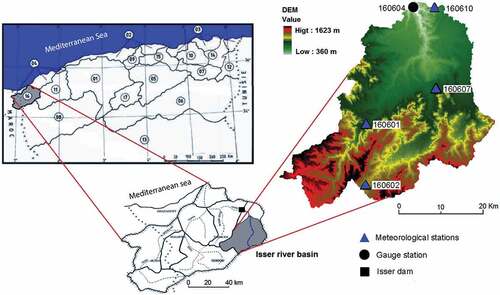
About one-third of the bedrock of this area consists of highly cemented conglomerates and ferruginous sandstones. These lithologies are located in the upper part of the catchment and form mountain ranges with smooth reliefs covered by shrubs. The bedrock in the rest of the study area consists of highly erodible and impermeable lithologies, mainly marls (Mazour 1992), that have generated a landscape divided into two main areas. In the foot of the reliefs formed by the conglomerates and sandstones, there is a dissected plain between 700 and 600 m a.s.l. covered by rain-fed crops. The incised part of this plain forms the lower part of the catchment where badlands and gentle hills cultivated with cereals and ligneous crops are common. The described region is characterized by very active erosion processes that have led to a rapid soil degradation but they are mainly concentrated in the lower part of the catchment, as exemplified by badlands (Boughalem et al. 2013, Chikh et al. 2019). Although the erosion problems are apparent, no action has been taken to combat this process in the area, nor have any conservation agricultural practices been applied to reduce its effects.

The former morphology gives the catchment an a priori torrential character. As shown in Table 1, the Isser River Basin shows an irregular flow regime with an average discharge of 1.22 m³ s⁻¹, maximum and minimum daily discharge of 295.40 and 0.004 m³ s⁻¹, respectively, and a runoff discharge peak value (ratio of discharge in the wettest month divided by the average annual discharge) of 200.

Table 1. Statistical values of the measured variables for the period 1988–2004. P: annual precipitation; SSC: suspended sediment concentration, Q_s: sediment flow; Q: runoff. SD: standard deviation.

	P (mm) (annual)	SSC (g/l) (daily)	$Q_s$(kg/s) (daily)	$Q\left({\mathrm{m}}^3/\mathrm{s}\right)$(avg. daily)	Consecutive days without SSC and Q measurements
Mean	322.93	0.97	13.92	1.22	3.13
SD	61.23	5.16	164.24	9.33	10.87
Min	269.94	0.01	0.0001	0.004	1.00
Max	409.71	67.20	3782.43	295.40	197.00

The torrential nature of the Isser River is linked to the semi-arid Mediterranean environment with a mean temperature of 17°C and a highly variable rainfall regime. Morsli et al. (2007) estimated mean annual precipitation of between 154 and 436 mm for the study area, which contrast with 1000 mm in the east of the country in very wet years. This assessment is close to the statistical results presented in Table 1 that were obtained by considering the data recorded at the study site and in the study period.

The National Agency of Hydraulic Resources of Algeria (ANRH) provided the main information to perform this study. The analysed measurements were recorded from 1988 to 2004 (Fig. 2). Daily precipitation data (Fig. 2(a)) was available from four meteorological stations (Fig. 1) which were equipped with basic equipment for measurement of rainfall by graduated cylinder, except for the station of Sidi Bounakhla (code: 160610), which included specific climatic variables such as wind velocity, air moisture and temperature. For potential hillslope erosion estimations of the USLE model, Chikh et al. (2019) completed this information with that from other 21 meteorological stations to estimate the spatial distribution of the erosivity factor, R. For this, an inverse distance weighting spatial interpolation, commonly used for the spatial interpolation method for precipitation (Lu and Wong 2008), was performed.

Figure 2. Available data for the study site. (a) Precipitation at four meteorological stations used as criteria for event selection and uncertainty analysis. (b) Flow measurements at the gauge station Sidi Abdelli. (c) Concentration and (d) sediment flow measured at the gauge station, and (e) periods without $\mathrm{S}\mathrm{S}\mathrm{C}$ and $Q$ data.

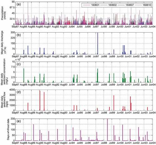
Water discharge was obtained from the hydrometric station of Sidi Abdelli Dam (code: 160604), where flow rates were obtained from water depth measurements recorded by an automated datalogger (Fig. 2(b)). This information was subsequently converted into flow by means of the calibrated depth/flow curve for the station’s cross-section. Suspended load (Fig. 2(c,d)) was determined following the methodology proposed by the ANRH and applied in all hydrological stations in Algeria. This methodology is based on manual sampling using a 1-L bottle and is based on personal evaluation of the flow regime and magnitude of the event. During floods, samples were taken at time steps of up to 30 min. depending on the velocity increase of the flow, while during stationary conditions measurements were carried out daily or every 2 days at 12:00 h (Terfous et al. 2001, Megnounif and Ghenim 2013, Achite and Ouillon 2016). Sediment concentration was later assessed by filtration method, weighing the sample after drying in an oven at 105°C for 30 min. and assuming that the addition of dissolved solids to the suspended sediment through evaporation was negligible (Khanchoul et al. 2012). Days without measurement due to the absence of events or failed campaign are shown in Fig. 2(e).

3 Methodology

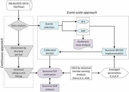
Figure 3 shows schematically the methodology followed in this work. As observed, the methods are organized under two different temporal scales in order to assess the impact on SSY during wet and humid periods. Distributed analysis of SDR and hysteresis loops at the event scale is performed for both periods. Also, sediment contribution based on the MUSLE parametric model is estimated at the event scale from seasonal remote sensing analysis. These approaches are described in detail in the following sections.

Figure 3. Flowchart illustrating the methodology developed for this work. Event-scale and continuous approaches are distinguished in order to assess seasonal SSY, SDR and basin–river interactions at the study site.

3.1 Analysis based on continuous measurements

The available data of SSC (g L⁻¹), sediment flow, $Q_s$ (kg s⁻¹), and water discharge (m³ s⁻¹) are analysed taking into account frequency, consecutive periods without data, and average, maximum, minimum and standard deviation of measurements. Periods of wet and dry seasons, defined as November–March and April–October, respectively, are identified and selected from the historical records. Periods longer than 3 days without data are ruled out for calculations. Accumulated precipitation during large gaps is analysed and the sensitivity of SSY estimates related to these gaps is assessed.

The continuous approach includes the fitting of rating curves for each period by means of the potential relationship $\mathrm{S}\mathrm{S}\mathrm{C}=\alpha Q^{\beta }$, where $\alpha$ and $\beta$ are the optimized parameters used to adjust this relationship. The coefficient of determination, $R^2$, and the correlation coefficient, $\rho$, are used to validate each adjustment and the statistical relationship between SSC and $Q$. Computation of SSY for the whole study period is obtained subsequently by considering seasonality and comparing it with the estimations based on a single rating curve fitted for the whole period.

3.2 Analysis based at event scale

The event-scale approach includes (1) the selection of rainfall events for dry and wet periods, (2) the seasonal analysis of hysteresis loops for the largest events and, (3) the regional calibration of the MUSLE model for each period.

3.2.1 Data analysis and events selection

Suspended-sediment events are selected for both wet and dry periods, taking into account rainfall patterns, runoff processes and suspended sediment dynamics, by applying the following criteria:

3.2.1.1 Event separation

Rainfall events are separated using an adaptation of the methodology implemented by Rahman et al. (2002) and Svensson et al. (2013) to the study area. This is achieved by considering a time span during which the average rainfall did not exceed a threshold of 2 mm d⁻¹, with intensities lower than 0.5 mm h⁻¹.

3.2.1.2 Event entity

Only events with SSC values greater than 100 mg L⁻¹, with a minimum event increase of 30 kg s⁻¹ and total contributions of 500 kg, are considered in order to limit the study to significant contribution for SSY estimates.

3.2.1.3 Rainfall–runoff relationship

In order to avoid interferences (baseflow events, anthropic influence, …) a runoff coefficient value – defined as a dimensionless coefficient relating the amount of runoff to the amount of precipitation during an event – greater than 0.1 was selected.

From these criteria, the maximum flow of the hydrograph, $Q_p$ (m³ s⁻¹), the volume of runoff, $V_q$ (m³) and the total mass of the outgoing sediment, $S_t$ (t), are estimated for each selected event. In addition, the contribution of these events is compared with the SSY results from continuous data assessment.

3.2.2 Hysteresis loop analysis

Of the selected events, those with higher water discharge are considered for hysteresis loop analysis of the dry and wet periods. It is assumed that the most important events, with relevant rainfall–runoff processes, mark the dynamics of sediment transport and hillslope–river relationships. The sense of the hysteresis loops provides insight into sediment sources and the mechanics of suspended sediment delivery (Jansson 2002). Five types of loop are distinguished: single-valued, clockwise, counter-clockwise, single-valued plus a loop and eight-shaped (Williams 1989). A single-valued loop presents discharge and sediment flow synchronized with continuous sediment supply (López-Tarazón and Estrany 2017). The clockwise sense is often related to in-channel sediment sources or sediment that is close to the catchment outlet (Walling and Webb 1982, Asselman et al. 2003, De Girolamo et al. 2015, Pietroń et al. 2015). Counter-clockwise loops indicate distant sediment sources, dominant hillslope erosion processes or differences in relative travel times between water and sediment waves (Williams 1989, Kurashige 1993, Seeger et al. 2004, De Girolamo et al. 2015). Eight-shaped loops are related to low soil moisture conditions and high-intensity rainfall events during summer (Zabaleta et al. 2007).

3.2.3 Seasonal calibration of the MUSLE model

The MUSLE model has been used to calculate the potential flux of soil erosion at the event scale in many different basins in the world (Sadeghi and Mizuyama 2007, Pandey et al. 2009, Zhang et al. 2009, Arekhi et al. 2011, Kumar et al. 2015). This parametric model is a modified version of the USLE (Wischmeier and Smith 1978), calibrated from approximately 778 individual storms in 18 basins of between 15 and 1500 ha. The basic and general equations for the model are as follows

(1) $S_y=a(V_q{Q}_p{)}^b\bar{K}\bar{L}S\bar{C}\bar{P}$(1)

where $a$ and $b$ are regional coefficients, with values of 11.8 and 0.56, respectively (Renard et al. 1997). The other factors in the equation $\bar{K}$, $\bar{L}S$, $\bar{C}$ and $\bar{P}$ are the averaged values of distributed USLE parameters. The erodibility factor $\bar{K}$ represents the susceptibility of a soil to erode, generally related to soil properties such as organic matter content, soil texture, soil structure and permeability. Topographic factor (slope and length of slope) represents the association of the steepness, $S$, and the length, $L$, of the slope and is generally obtained from the digital elevation model (DEM). The mean values of these factors were estimated from the maps generated in a previous investigation (Chikh et al. 2019). The distributed estimation of the tillage practices factor, $\bar{P}$, is associated with important sources of uncertainty related to the difficulty in predicting how microtopography affects hydraulics and flow paths (Renard et al. 1991). In this study, $\bar{P}$is assumed to be equal to 1.00, as previously reported (Wang et al. 2003, Smith et al. 2007, Oliveira et al. 2015, Kuo et al. 2016). Since the vegetation cover factor $C$ changes in time, its estimation is performed by considering the vegetation cover dynamic, assessed from the available satellite images by means of the normalized differential vegetation index, NDVI (Karaburun 2010). Landsat remote sensing images were downloaded from the US Geological Survey database, analysed and corrected. Estimation of NDVI was subsequently performed using the spectral reflectance acquired in the red ($\mathrm{R}\mathrm{E}\mathrm{D}$) and near-infrared ($\mathrm{N}\mathrm{I}\mathrm{R}$) wavelengths by (Rouse et al. 1974):

(2) $\mathrm{N}\mathrm{D}\mathrm{V}\mathrm{I}=\left(\mathrm{N}\mathrm{I}\mathrm{R}-\mathrm{R}\mathrm{E}\mathrm{D}\right)/\left(\mathrm{N}\mathrm{I}\mathrm{R}+\mathrm{R}\mathrm{E}\mathrm{D}\right)$(2)

Factor $C$ is estimated as follows:

(3) $C=\mathrm{e}\mathrm{x}\mathrm{p}\left(-\omega \frac{\mathrm{N}\mathrm{D}\mathrm{V}\mathrm{I}}{\theta -\mathrm{N}\mathrm{D}\mathrm{V}\mathrm{I}}\right)$(3)

where $\omega$ and $\theta$ are dimensionless parameters that determine the shape of the curve relating NDVI to C. This scaling approach gives better results than assuming a linear relationship and values of 2 and 1 for $\omega$ and $\theta$, respectively (Van der Knijff et al. 2000). This model has been applied successfully in Mediterranean environments (Kouli et al. 2009) and has been used to evaluate the $C$ factor by many researchers in other areas (e.g. Prasannakumar et al. 2012, Nyesheja et al. 2018, Thomas et al. 2018). Based on this analysis, values of $\bar{C}$ are used for selected events in the dry and wet seasons.

The MUSLE model depends on multiple factors that present a great spatial and temporal variability from different points of view: rainfall regime, basin relief and geology, edaphic heterogeneity, besides the anthropic influence (Prado-Hernández et al. 2017). In this sense, Williams (1975) indicated that calibration of parameters $a$ and $b$ is essential in order to represent correctly the erosive dynamic of the study area. Furthermore, several studies have highlighted the need for calibration in order to take account of the local conditions (Avanzi et al. 2008, Noor et al. 2012, Sadeghi et al. 2013, Cariello et al. 2014, Prado-Hernández et al. 2017) and the influence of the SDR (Chen and Mackay 2004) of the studied basin. From a global comparative study, Sadeghi et al. (2014) carried out an exhaustive analysis of 49 basins and bounded the values of coefficient $a$ and exponent $b$ between 0.001 and 6.38 and 0.081 and 1.12 respectively, which indicates the wide range of calibration values.

In this work, calibration of the original MUSLE parameters is considered, as well as the adjustment of a global factor, $F_M$, which allows us to evaluate the deviation of the original version of the model. To this end, the process of calibration evaluates the best value of Nash–Sutcliffe model efficiency coefficient (NSE), which is commonly used to assess the predictive relationships of hydrological models as follows (Nash and Sutcliffe 1970):

(4) $NSE=1-\frac{{{\sum }_{i=1}^n(O_i-S_{{ }_i})}^2}{{\sum }_{i=1}^n{(O_i-\bar{S})}^2}$(4)

where $O_i$ represent the observed values, $S_i$ are the simulated values, $\bar{S}$ represents the averaged of the observed values and n is the number of samples.

3.3 Estimation and comparison of the erosive rate

Both approaches based on continuous and event-scale calculations of sediment flow are analysed in terms of seasonal variability of sediment yield. In addition, comparison between estimated sediment flow and potential erosion allowed us to analyse the sediment delivery ratio (SDR), defined as the ratio between estimated sediment yield and the gross erosion on a watershed (Julien 2010). This value represents the efficiency of sediment transport from the drainage network of the basin and is generally associated with different parameters such as the area, the average basin slope, its relief, or the density of the drainage network (Bagarello et al. 1991). To estimate the SDR, the potential soil loss estimated previously with the RUSLE model (Chikh et al. 2019) is compared with sediment flow measured downstream. This information is also used to calibrate the distributed SDR model proposed by Borselli et al. (2008):

(5) $\mathrm{S}\mathrm{D}\mathrm{R}=\frac{\mathrm{S}\mathrm{D}{\mathrm{R}}_{\mathrm{m}\mathrm{a}\mathrm{x}}}{1+{\mathrm{e}}^{\frac{\mathrm{I}{\mathrm{C}}_0-\mathrm{I}{\mathrm{C}}_i}{\lambda }}}$(5)

where $\mathrm{S}\mathrm{D}{\mathrm{R}}_{\mathrm{m}\mathrm{a}\mathrm{x}}$ is the maximum theoretical $\mathrm{S}\mathrm{D}\mathrm{R}$, set to an average value of 0.8 (Vigiak et al. 2012), $\mathrm{I}{\mathrm{C}}_0$ and $\lambda$ are calibration parameters and the landscape metric or connectivity index, $\mathrm{I}{\mathrm{C}}_i$, is defined as:

(6) $\mathrm{I}{\mathrm{C}}_i=\mathrm{l}\mathrm{o}{\mathrm{g}}_{10}\left(\frac{\overline{S_{\mathrm{u}\mathrm{p}}}\overline{C_{\mathrm{u}\mathrm{p}}}\sqrt{A_{\mathrm{u}\mathrm{p}}}}{{\sum }_i\frac{d_i}{C_i{S}_i}}\right)$(6)

where $\overline{C_{\mathrm{u}\mathrm{p}}}$ is the average $C$ factor of the USLE model, provided by the remote sensing analyses, of the upslope contributing area, $A_{\mathrm{u}\mathrm{p}}$ (m²); $\overline{S_{\mathrm{u}\mathrm{p}}}$ is the average slope gradient (mm⁻¹) of the upslope contributing area; $d_i$ is the length of the flow path along the ith cell according to the steepest downslope direction; and $C_i$ and $S_i$ are the $C$ factor and the slope gradient of the ith cell, respectively. A Python code is developed which uses the DEM and the value of parameters $C$ and $S$ as basic input for the calculation of the upstream accumulated average values and the flow path length downstream.

4 Results and discussion

From 17 years of measurements, differences between frequency and continuity on data acquisition clearly separate the meteorological and hydrological variables. Rainfall presented daily continuous data without gaps, while SSC and $Q$ data series showed important discontinuities. For this case, periods exceeding 3 days without measurement were discarded for the analyses.

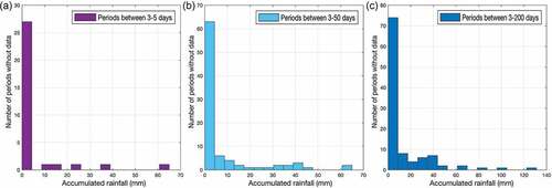
By examining the historical data series, 106 gaps were observed with 2623 days exceeding the threshold of 3 days of continuous data (43% of the whole period). From these, 73% corresponded to periods of more than 50 consecutive days without measure, with a total of 18 gaps. The analysis of the accumulated precipitation during these periods is shown in Fig. 4 which presents different time windows without measurements (2–5, 3–50 and 3–200 days). As observed, the occurrence of relevant events, with accumulated rain of more than 35 mm and gaps of between 3 and 5 days, is limited to two events. Longer intervals without data, up to 197 days, presented seven periods with accumulated rainfall greater than 40 mm and values of between 25 and 45 mm d⁻¹. The percentage of days without rainfall or with accumulated values of less than 5 mm during gaps was 70%. Consequently, this study was based on 1958 samples of SSC, sediment flow and runoff representing 3522 days (9.65 years). A total of 1836 days without significant SSC contributions are assumed and up to 787 days without measurement were estimated, from which up to seven rainfall events of significant intensity were recorded. Table 1 shows the values of mean, standard deviation (SD), maximum (max) and minimum (min) values of the measured variables, as well as the days without measurements. As observed, the minimum and maximum values highlight the important variability of SSC, sediment flow and runoff. It is important to note that the intense event registered in September 1997, with discharge of almost 300 m³ s⁻¹, was discarded from the analysis as errors of SSC were reported.

Figure 4. Accumulated rainfall with respect to the number of periods without SSC and $Q$ measurements for different time windows: (a) 3–5 days, (b) 3–50 days and 3–200 days.

From the analysed data, the relationship between SSC and $Q$ (Fig. 5(a–c)), shows a good correlation based on the continuous approach for the whole period, with $\alpha$ = 126, $\beta$ = 0.76, R² = 0.60 and $\rho$ = 0.74; and for the dry and wet periods, with respective values of 2777.2, 0.67, 0.71 and 0.80, and 1418.6, 0.76, 0.6 and 0.75. In addition, the relationship in the three cases presented p values of 0.05, which confirms the significant statistical correlation between SSC and $Q$. Figure 5(d) presents the comparison of the adjusted seasonal data in the study site with other studies in the Mediterranean area. As observed, the study area has a very similar dynamic, in the upper range, to other Mediterranean rivers (Farguell and Sala 2006, Mano et al. 2009, Khanchoul et al. 2009, De Girolamo et al. 2015, Selmi and Khanchoul 2016), and only below flash flood episodes at the Eshtemoa River (Alexandrov et al. 2007). As shown in Fig. 5(d), the northeastern part of the Iberian Peninsula presents much larger variations of SSC–Q relationship, as reported by Batalla and Sala (1994) and Farguell and Sala (2006). In the Isser River Basin, significant differences were observed between the values of the parameters adjusted for wet and dry periods. The coefficient $\alpha$ fitted for the dry period is almost double that for the wet one, while the coefficient $\beta$ is higher in wet periods, marking the value of the whole analysis (Fig. 5(a)). It is important to mention that the number of samples in the wet period (1393) is considerably higher than that in the dry one (468), which explains its dominance in the global analysis. These results highlight the erosive power of events during the dry period and a slightly greater variation of SSC with water discharge during wet periods.

Figure 5. Relationship between SSC and water discharge from measured samples for (a) the whole period, and for (b) dry and (c) wet periods. The adjustment based on the $\mathrm{S}\mathrm{S}\mathrm{C}=\alpha Q^{\beta }$ relationship, with fitted parameters and the coefficient of determination. (d) Comparison with other Mediterranean environments is shown based on the following sources: Arbucies River: .Batalla and Sala (1994); Anoia River: Farguell and Sala (2006); Celone River: De Girolamo et al. (2015); Asser River: Mano et al. (2009); Mellah River: Khanchoul et al. (2009); Mellegue River: Selmi and Khanchoul (2016); and Eshtemoa River: Alexandrov et al. (2007).

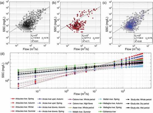
It is important to note the relationship between these results and other nearby basins in the northwest of Algeria. The adjustments obtained here are in line with the dynamics of transport on the Mellegue River (Selmi and Khanchoul 2016) and both much greater than those reported for the Mellah River (Khanchoul et al. 2009). This highlights the great variability in erosion and transport processes in Mediterranean environments.

The potential fit of this relationship allowed us to estimate SSY based on available measurements of water discharge, mass integration of SSC contributions, periods without gaps (with a total of 9.65 years), and the area of study site. Figure 6(a) shows the accumulated sediment flow estimated from the fitted relationship from the measurements, from the potential fitted relationship for the whole period and from the potential fitted relationship by distinguishing between dry and wet periods. The result provides a range of SSY of between 7.94 and 8.25 t ha⁻¹ year⁻¹, when comparing calculations from data and potential models based on seasonality. This range is very similar (8.3 t ha⁻¹ year⁻¹) when the whole period is considered and seasonality is not take into account. Figure 6(b) shows the effects of less restrictive consideration of stationary conditions, or periods without measurements, on SSY estimation. As observed, for the three analysed scenarios, the value of SSY increases to maxima of 10.3, 11.7 and 9.8 t ha⁻¹ year⁻¹ under seasonal-based, measures-based and global-based approaches, respectively. In turn, the accumulated precipitation increased with greater values of $\mathrm{d}d$, which shows the occurrence of events during these gaps, as reported previously, increasing uncertainty of these estimations.

Figure 6. (a) Cumulative water discharge and sediment flow from measurements and rating curve estimations. Pulses of significant events and their impacts on sediment transport are clearly identified. (b) Resulting values of SSY obtained by considering increasing time windows without SSC and $Q$ measurements, assuming stationary conditions of flow.

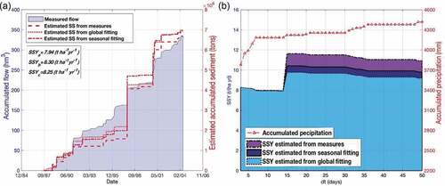
Considering the SSY results for each season separately, values of 4.3 and 13.2 t ha⁻¹ year⁻¹ are obtained for the wet and dry periods, respectively, from both measurements and rating curve. This range could vary if we consider the influence of extreme events such as the one of 300 m³ s⁻¹, discarded in this work due to measurement errors. By assuming a triangular sedimentograph lasting 1 day, and the estimated rating curves, the value of SSY could increase to 1.32 t ha⁻¹ year⁻¹. This represents 10% and 30% higher SSY for dry and wet periods respectively, and highlights both the importance of extreme pulses and the need for their correct measurement.

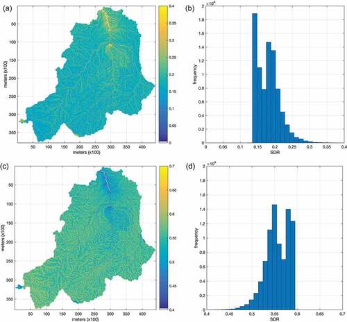
These seasonal differences were previously reported in Chikh et al. (2019), who reported potential erosion rates with RUSLE approaches associated with changes in crop cover during each season. If we consider such results based on remote sensing analysis, the SSY ranges from 23.5 to 25 t ha⁻¹ year⁻¹ (for wet and dry periods, respectively). Thus, the resulting SDR can be estimated as 0.2 and 0.52, respectively. In both cases, these values are higher than those previously reported in potential empirical relationships based on $A-\mathrm{S}\mathrm{D}\mathrm{R}$ relationships (Ferro and Minacapilli 1995, Lu et al. 2006). This highlights the effectiveness of the sediment transport, especially during dry periods. The absence of corrective measures, represented by the USLE P factor, and the land cover dynamics, could explain the extraordinary transport effectiveness in the study area.

Furthermore, Fig. 7 show distributed values of SDR obtained following the methodology proposed by Borselli et al. (2008). As observed, there is a notable contrast between wet and dry periods for calibration parameters of $\lambda =3.8$, with $\mathrm{I}{\mathrm{C}}_0=0.5$, for wet periods, values that are similar to those reported by Vigiak et al. (2012), and $\lambda =-6.3$ with $\mathrm{I}{\mathrm{C}}_0=0.5$ for dry periods. The sign of $\lambda$ accounts for continuous increasing ($\lambda >0$) or decreasing ($\lambda <0$) SDR along with the channel network. Based on this, the calibration results point to an inversion of effectiveness of sediment transport between rivers and hillslopes during dry periods, when channels tend to have less transport efficiency than hillslopes. This effect could be related to differences in saturation conditions of the edaphic profile of hillslopes and channels between seasons, which affect runoff processes. According to these results, although the mean value of SDR in dry periods is higher, the efficiency along the drainage network is similar or greater in wet periods, which is in line with the $\beta$ values obtained from rating curve adjustments. It is important to highlight the high sensitivity of $\lambda$ regarding $\mathrm{I}{\mathrm{C}}_0$, which can be considered landscape independent (Vigiak et al. 2012).

Figure 7. Distributed values of SDR, obtained by implementing the methodology of Borselli et al. (2008), and associated histograms for: (a)–(b) wet and (c)–(d) dry seasons.

At the event scale, a total of 25 and 59 rainfall events were selected for dry and wet periods, respectively, following the methodology and criteria described above. For each event, we calculated sediment flow and the total flow contributions. Of these, only the largest events were chosen for hysteresis analysis, in descending order of peak flow, discarding those that did not present a minimum of 4 days of consecutive measurements. It is assumed that intense events dominate erosion and transport dynamics in the study area.

Finally, 12 intense events were selected for the analysis. Figure 8 and Table 2 show hysteresis loop results and a summary of period and season of each event. As shown, the events selected in the wet period (2, 4, 6, 8, 9, 10 and 12) mostly presented clockwise loops, except for events 8 and 12, whose dates are close to the dry season. In contrast, most of the events from dry period (1, 3, 5, 7 and 11) presented counter-clockwise loops, with the exception of event 5. These results coincide with the seasonal patterns described in previous works (e.g. Zabaleta et al. 2007). If we consider the annual distribution in which these 12 events have been selected, a certain cycle, similar to that described by Rovira and Batalla (2006), is identified. This cyclical behaviour could be separated into two phases: (1) a phase of “sediment preparation”, in winter and summer, and (2) a phase of sediment transport and exhaustion around spring and autumn. During this second phase, when the sediment transport occurs, the events selected in late winter and spring were mostly clockwise, except for events 7 and 12, with low discharge peaks of 23 and 28 m³ s⁻¹, respectively. This result could be related to a quick response of sediment accumulated in the channel, as previously described (Lenzi and Marchi 2000, Jansson 2002). The events measured in late summer and autumn, predominantly counter-clockwise, presented considerably higher sediment peak discharges (4–7 10⁴ mg L⁻¹). This could be associated with sediment contributions from all over the catchment, intense rainfall events or the higher hillslope erodibility (Seeger et al. 2004, Abdelwahab et al. 2014).

Table 2. Summary of seasons and hysteresis loop sense for the events selected. Shaded areas indicate the dry period and unshaded the wet period. The symbols and indicate clockwise and counter-clockwise direction, respectively.

Month	12	1	2	3	4	5	6	7	8	9	10	11
	Winter			Spring			Summer			Autumn
1
2
3
4
5
6
7
8
9
10
11
12

Figure 8. Hysteresis curves for the 12 largest events for which data were available in the historical data. D and W refer to dry and wet periods, respectively. Dots mark the loop direction (from dark blue to yellow).

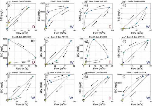
These results, which fit the soil degradation patterns described for the study area, also support the differences between periods analysed from rating curves and distributed SDR values.

The outgoing sediment from the 84 rainfall events was close to 1.58 × 10⁶ t, which represents the 23.7% of the estimated value for the whole period, with a duration of between 1 and 4 days. If we consider the 10 largest daily events, 6 in wet periods and 4 in dry periods, their total mass amount represented the 34.6% of the contributions during the study period. This percentage is close to the average value obtained by González‐Hidalgo et al. (2010) when considering the 10 largest events of 1314 basins throughout the USA. However, in that study, Mediterranean environments such as California presented values of up to 60%. It is important to highlight the limitations in this study related to the intense events that occurred during periods without measurements, so the result of 34.6% could be higher.

Furthermore, the volume of water ($V_q$) and the maximum flow ($Q_p$) for each selected event were assessed. Figure 9 shows the results by comparing the total mass obtained by modelling with MUSLE and by measuring for each event. As observed, the total mass calculated by the MUSLE model is strongly correlated with the outgoing sediment mass of the selected events ($R^2$= 0.95). Despite this, a clear overestimation of the MUSLE model is observed when the original coefficient $a$ and exponent $b$ are used, as has been previously reported (McConkey et al. 1997, Sadeghi and Mizuyama 2007, Arekhi et al. 2011). The values of these parameters, as well as for the global factor, $F_M$, which affects the original version of the MUSLE model, were calibrated based on the information of selected events. Figure 10(a) shows $\mathrm{N}\mathrm{S}\mathrm{E}$ values for $F_M$ results, distinguishing between wet and dry periods. Figure 10(b) and (c) shows the NSE values obtained for the coefficient $a$ and the exponent $b$ for wet and dry periods, respectively, in which the ranges of optimal values of both parameters are clearly identified. Table 3 summarizes these results based on the maximum values of NSE.

Table 3. Results of the MUSLE model parameters calibrated at the study area, a and b, and the global factor, $F_M$ for wet and dry periods. NSE: Nash–Sutcliffe efficiency criterion.

		$a$	$b$	$F_M$	NSE
Wet period	MUSLE original optimized	11.8	0.56	0.20	0.95
	MUSLE optimized	0.43	0.64	1	0.95
Dry period	MUSLE original optimized	11.8	0.56	0.39	0.87
	MUSLE optimized	0.05	0.79	1	0.91

Figure 9. Relationship between the estimated contribution of sediment measured for each event and that estimated with the MUSLE model for wet (blue triangle) and dry (red dot) periods.

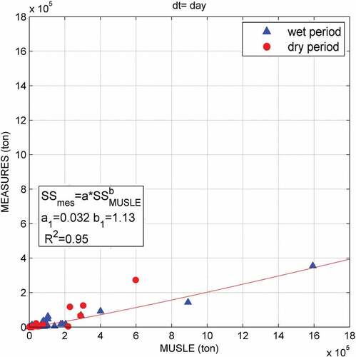
Figure 10. (a) Performance measured by NSE values of the global factor of MUSLE correction, $F_M$, for wet and dry periods. (b) Wet period and (c) dry period NSE values for the coefficient a and exponent b of the MUSLE model regionalized for the study area.

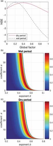
As shown in Fig. 10(a), the optimal values of $F_M$ are 0.2 and 0.4 for wet and dry periods, respectively, which highlights the significant overestimation of the model in wet and dry periods, estimated as 80% and 60%, respectively. This result is again notable, indicating the importance of sediment flow at the event scale in dry periods despite its lower frequency. The calibration MUSLE parameters (Fig. 10(b,c)) support these differences with a shift toward lower values of the exponent $b$ in the wet period when compared to the dry one. This implies a lower sediment yield capacity for events occurring in the wet period compared to those of the dry period, which fits with the results obtained in this research. The coefficient $a$ presented a very wide range of optimal values in both cases, ranging from 0.01 to 20, higher than the range of values estimated by Sadeghi et al. (2014) from comparison of 49 researches. On the contrary, the shorter range of values of the exponent $b$, on between 0.4 and 0.7, was close to the mean value estimated in such research.

5 Conclusions

The data analysed in this work allow the estimations of soil loss attributed to seasonality from 17 years of suspended sediment monitoring. Variations in erosion and transport dynamics during dry and wet periods were observed from different approaches.

The fitted $\mathrm{S}\mathrm{S}\mathrm{C}$–$Q$ rating curves showed a good relationship and correlation, presenting similar transport dynamics, within the upper range, compared to other Mediterranean rivers, especially during the dry season. The relationship obtained, allowed us to make a more contrasted estimation of SSY, assessed as between 8 and 8.3 t ha⁻¹ year⁻¹ from measures and rating curve fitting based on global or seasonal approaches. The analysis also allowed us to identify significant differences in seasonal SSY, estimated at 4.3 and 13 t ha⁻¹ year⁻¹ for wet and dry periods, respectively. This differentiated erosive dynamics responds to changes in crop cover during each season as reported previously for the study area.

Furthermore, these results allowed us to compare differences in sediment delivery ratio, estimated as 0.2 and 0.55 for wet and dry seasons, respectively. Distributed SDR analysis pointed to an increase in transport effectiveness, especially within the hillslopes during dry seasons and at the channel network during wet periods.

At the event scale, the selection of relevant rainfall events allowed us to contrast seasonality on sediment transport dynamics. The study of the 12 largest events available in the dry and wet periods confirmed differences in hysteresis loops related to seasonality, as described for other environments, not only in Mediterranean regions. While for dry periods most of the selected events presented anti-clockwise loops, wet periods presented clockwise ones. These results could be related to sediment stored at the channel during moderate intensity and recurrent episodes of wet periods, and higher soil erodibility, lower land cover and severe hillslope erosion processes during dry periods.

The total contribution of the 84 selected events represents 25% of the estimated SSY. If we consider the 10 largest daily events, their total amount of sediment corresponded to a fraction of 34.6% of the total sediment output, which is low when compared with other Mediterranean environments. The application of the MUSLE model with its original parameters showed an overestimation of sediment contribution for both dry and wet periods (of 60% and 80%, respectively). Model calibration showed values of coefficient $a$ and exponent $b$ for the dry and humid periods that pointed to the severity of the events that occurred during the dry period.

The results of this research highlight the importance of seasonality in erosion and sediment transport processes, which is especially relevant in Mediterranean environments where future climate scenarios based on global circulation models predict an increase in frequency and intensity of events in dry periods (Alpert et al. 2002).

Acknowledgements

The authors would like to thank the National Agency for Hydraulic Resources of Algeria (ANRH) for the availability of data that has allowed this work to be developed. The first author also thanks the collaboration of the Department of Geodynamics and the Andalusian Institute for Earth System Research (IISTA) of the University of Granada. The authors wish to sincerely thank the anonymous reviewers whose comments greatly improved the quality of this paper.

Disclosure statement

No potential conflict of interest was reported by the authors.

Additional information

Funding

This research was partially supported by the project [CGL2015-67130-C2-1-R] Spanish Ministry of Economy and Competitiveness (MINECO).

References

- Abdelwahab, O.M., et al., 2014. Effectiveness of alternative management scenarios on the sediment load in a Mediterranean agricultural watershed. Journal of Agricultural Engineering, 45 (3), 125–136. doi:10.4081/jae.2014.430.
- Achite, M. and Ouillon, S., 2016. Recent changes in climate, hydrology and sediment load in the Wadi Abd, Algeria (1970–2010). Hydrology and Earth System Sciences, 20, 1355–1372. doi:10.5194/hess-20-1355-2016.
- Alexandrov, Y., Laronne, J.B., and Reid, I., 2007. Intra-event and inter-seasonal behaviour of suspended sediment in flash floods of the semi-arid northern Negev, Israel. Geomorphology, 85 (1–2), 85–97. doi:10.1016/j.geomorph.2006.03.013.
- Alpert, P., et al., 2002. The paradoxical increase of Mediterranean extreme daily rainfall in spite of decrease in total values. Geophysical Research Letters, 29, 11. doi:10.1029/2001GL013554.
- Arekhi, S., Shabani, A., and Alavipanah, S.K., 2011. Evaluation of integrated KW-GIUH and MUSLE models to predict sediment yield using geographic information system (GIS) (Case study: kengir watershed, Iran). African Journal of Agricultural Research, 6, 4185–4198.
- Asselman, N.E., Middelkoop, H., and Van Dijk, P.M., 2003. The impact of changes in climate and land use on soil erosion, transport and deposition of suspended sediment in the river Rhine. Hydrological Processes, 17, 3225–3244. doi:10.1002/hyp.1384.
- Avanzi, J.C., et al., 2008. Calibration and application of the MUSLE model in a coastal watershed in the Tabuleiros Brazilian (Calibração e aplicação do modelo MUSLE em uma microbacia hidrográfica nos Tabuleiros Costeiros brasileiros). Revista Brasileira De Engenharia Agrícola E Ambiental, 12, 563–569. doi:10.1590/S1415-43662008000600001.
- Bagarello, V., Ferro, V., and Giordano, G., 1991. Contribution to the evaluation of the Williams outflow factor and the solid yield coefficient for some Sicilian watersheds (Contributo alla valutazione del fattore di deflusso di Williams e del coefficiente di resa solida per alcuni bacini idrografici siciliani). Rivista Di Ingegneria Agraria, 4, 238–251.
- Balla, F., et al., 2017. Hydro-sedimentary flow modelling in some catchments Constantine highlands, case of Wadis Soultez and Reboa (Algeria). Journal of Water and Land Development, 34, 21–32. doi:10.1515/jwld-2017-0035.
- Barthes, B. and Roose, E., 2002. Aggregate stability as an indicator of soil susceptibility to runoff and erosion; validation at several levels. Catena, 47, 133–149. doi:10.1016/S0341-8162(01)00180-1.
- Batalla, R.J. and Sala, M. 1994. Temporal variability of suspended sediment transport in a Mediterranean sandy gravel-bed river. In: L.J. Olive, R.J. Loughran, and J.A. Kesby, eds. Variability in stream erosion and sediment transport (Proceedings of the Canberra symposium, December 1994). Wallingford, UK: International Association of Hydrological Sciences, IAHS Publ. no. 224, 299–306. https://iahs.info/uploads/dms/iahs_224_0299.pdf [Accessed 11 January 2020].
- Bernoux, M., et al., 2006. Cropping systems, carbon sequestration and erosion in Brazil, a review. Agronomy for Sustainable Development, 26, 1–8. doi:10.1051/agro:2005055.
- Borselli, L., Cassi, P., and Torri, D., 2008. Prolegomena to sediment and flow connectivity in the landscape: a GIS and field numerical assessment. Catena, 75 (3), 268–277. doi:10.1016/j.catena.2008.07.006.
- Bouchetata, A. and Bouchetata, T., 2006. Propositions d’aménagement du sous-bassin-versant de l’oued Fergoug (Algérie) fragilisé par des épisodes de sécheresse et soumis à l’érosion hydrique. Science et changements planétaires - Sécheresse, 17, 415–424.
- Boughalem, M., Abdellaoui, A., and Moussa, K., 2014. Variabilité spatiale de l’infiltrabilité sur les versants marneux de l’Isser-Tlemcen (Algérie). Revista De Geomorfologie, 16, 71–77.
- Boughalem, M., et al., 2013. Evaluation par analyse multicritères de la vulnérabilité des sols a l’érosion: cas du bassin versant de l’Isser–Tlemcen–Algérie. Analele Universitatii Bucuresti, 1, 5–26.
- Boultif, M. and Benmessaoud, H., 2017. Using climate-soil-socioeconomic parameters for a drought vulnerability assessment in a semi-arid region: application at the region of El Hodna, (M’sila, Algeria). Geographica Pannonica, 21, 142–150. doi:10.5937/GeoPan1703142B.
- Buffington, J.M. and Montgomery, D.R., 2013. Geomorphic classification of rivers. In: J. Shroder and E. Wohl, eds. Treatise on geomorphology; fluvial geomorphology. Vol. 9. San Diego, CA: Academic Press, 730–767.
- Cariello, B., et al., 2014. Application and calibration of the modified universal soil loss equation to estimate the sediment yield in a small Amazon catchment. Sylwan Journal, 158, 347–359.
- Chalov, S., et al., 2017. A toolbox for sediment budget research in small catchments. Geography, Environment, Sustainability, 10 (4), 43–68. doi:10.24057/2071-9388-2017-10-4.
- Chen, E. and Mackay, D.S., 2004. Effects of distribution-based parameter aggregation on a spatially distributed agricultural nonpoint source pollution model. Journal of Hydrology, 295, 211–224. doi:10.1016/j.jhydrol.2004.03.029.
- Chikh, H.A., Habi, M., and Morsli, B., 2019. Influence of vegetation cover on the assessment of erosion and erosive potential in the Isser marly watershed in northwestern Algeria-comparative study of RUSLE and PAP/RAC methods. Arabian Journal of Geosciences, 12, 154. doi:10.1007/s12517-019-4294-3.
- Church, M. and Slaymaker, O., 1989. Disequilibrium of holocene sediment yield in glaciated British Columbia. Nature, 337, 452–454. doi:10.1038/337452a0.
- De Girolamo, A.M., Pappagallo, G., and Porto, A.L., 2015. Temporal variability of suspended sediment transport and rating curves in a Mediterranean river basin: the Celone (SE Italy). Catena, 128, 135–143. doi:10.1016/j.catena.2014.09.020.
- Faran Ali, K. and de Boer, D.H., 2008. Factors controlling specific sediment yield in the upper Indus river basin, northern Pakistan. Hydrological Processes, 22, 3102–3114. doi:10.1002/hyp.v22:16.
- Farguell, J. and Sala, M., 2006. Seasonal trends of suspended sediment concentration in a Mediterranean basin (Anoia river, NE Spain). In: P.N. Owens and A.J. Collins, eds. Soil erosion and sediment redistribution in river catchments: measurement, modelling and management. Cranfield, 85.
- Ferreira, V. and Panagopoulos, T., 2012. Predicting soil erosion risk at the Alqueva dam watershed. Faro: CIEO-Research Centre for Spatial and Organizational Dynamics, University of Algarve, (Technical Report No. 2012-4).
- Ferro, V. and Minacapilli, M., 1995. Sediment delivery processes at basin scale. Hydrological Sciences Journal, 40, 703–717. doi:10.1080/02626669509491460.
- Ghanam, M., 2003. La désertification au Maroc-Quelle stratégie de lutte. In: 2nd FIG regional conference marrakech, December Morocco, 2–5.
- González‐Hidalgo, J.C., et al., 2010. Contribution of the largest events to suspended sediment transport across the USA. Land Degradation and Development, 21 (2), 83–91. doi:10.1002/ldr.897.
- Gregory, K.J. and Walling, D.E., 1973. Drainage basin form and process: a geomorphological approach. London: Hodder Arnold.
- Jansson, M.B., 2002. Determining sediment source areas in a tropical river basin, Costa Rica. Catena, 47 (1), 63–84. doi:10.1016/S0341-8162(01)00173-4.
- Julien, P.Y., 2010. Erosion and sedimentation. Cambridge, UK: Cambridge University Press.
- Karaburun, A., 2010. Estimation of c factor for soil erosion modeling using NDVI in Buyukcekmece watershed. Ozean Journal of Applied Sciences, 3, 77–85.
- Khanchoul, K., Altschul, R., and Assassi, F., 2009. Estimating suspended sediment yield, sedimentation controls and impacts in the Mellah Catchment of Northern Algeria. Arabian Journal of Geosciences, 2 (3), 257–271. doi:10.1007/s12517-009-0040-6.
- Khanchoul, K., et al., 2012. Estimation of suspended sediment transport in the Kebir drainage basin, Algeria. Quaternary International, 262, 25–31. doi:10.1016/j.quaint.2010.08.016.
- Kinnell, P. and Risse, L., 1998. USLE-M: empirical modeling rainfall erosion through runoff and sediment concentration. Soil Science Society of America Journal, 62, 1667–1672. doi:10.2136/sssaj1998.03615995006200060026x.
- Kouli, M., Soupios, P., and Vallianatos, F., 2009. Soil erosion prediction using the revised universal soil loss equation (RUSLE) in a GIS framework, Chania, Northwestern Crete, Greece. Environmental Geology, 57, 483–497. doi:10.1007/s00254-008-1318-9.
- Kumar, P.S., Praveen, T., and Prasad, M.A., 2015. Simulation of sediment yield over un-gauged stations using MUSLE and fuzzy model. Aquatic Procedia, 4, 1291–1298. doi:10.1016/j.aqpro.2015.02.168.
- Kuo, K.T., Sekiyama, A., and Mihara, M., 2016. Determining C factor of Universal Soil Loss Equation (USLE) based on remote sensing. International Journal of Environmental and Rural Development, 7, 154–161.
- Kurashige, Y., 1993. Mechanism of suspended sediment supply to headwater rivers and its seasonal variation in west central Hokkaido, Japan. Japanese Journal of Limnology, 54, 305–315. doi:10.3739/rikusui.54.305.
- Lenzi, M.A. and Marchi, L., 2000. Suspended sediment load during floods in a small stream of the Dolomites (northeastern Italy). Catena, 39 (4), 267–282. doi:10.1016/S0341-8162(00)00079-5.
- López‐Tarazón, J.A. and Estrany, J., 2017. Exploring suspended sediment delivery dynamics of two Mediterranean nested catchments. Hydrological Processes, 31 (3), 698–715. doi:10.1002/hyp.11069.
- Lu, G.Y. and Wong, D.W., 2008. An adaptive inverse-distance weighting spatial interpolation technique. Computers & Geosciences, 34, 9. doi:10.1016/j.cageo.2007.07.010.
- Lu, H., Moran, C.J., and Prosser, I.P., 2006. Modelling sediment delivery ratio over the Murray Darling basin. Environmental Modelling & Software, 21, 1297–1308. doi:10.1016/j.envsoft.2005.04.021.
- Mano, V., et al., 2009. Assessment of suspended sediment transport in four alpine watersheds (France): influence of the climatic regime. Hydrological Processes, 23 (5), 777–792. doi:10.1002/hyp.v23:5.
- Mazour, M., 1992. Les facteurs de risque de l’érosion en nappe dans le bassin versant d’isser, Tlemcen, Algérie. Bulletin-réseau Erosion, 1, 300–313.
- McConkey, B., et al., 1997. Sediment yield and seasonal soil erodibility for semiarid cropland in western Canada. Canadian Journal of Soil Science, 77, 33–40. doi:10.4141/S95-060.
- Meddi, M., Talia, A., and Martin, C., 2009. Évolution récente des conditions climatiques et des écoulements sur le bassin versant de la Macta (Nord-Ouest de l’Algérie). Physio-Géo, 3, 61–84. doi:10.4000/physio-geo.
- Megnounif, A. and Ghenim, A., 2013. Influence des fluctuations hydro-pluviométriques sur la production des sédiments: cas du bassin de la Haute Tafna. Journal of Water Science, 26, 53–62.
- Megnounif, A., Terfous, A., and Bouanani, A., 2003. Production et transport des matières solides en suspension dans le bassin versant de la Haute-Tafna (Nord-Ouest Algérien). Journal of Water Science, 16, 369–380.
- Millares, A., Díez-Minguito, M., and Moñino, A., 2019. Evaluating gullying effects on modeling erosive responses at basin scale. Environmental Modelling & Software, 111, 61–71. doi:10.1016/j.envsoft.2018.09.018.
- Millares, A. and Moñino, A., 2018a. Sediment yield and transport process assessment from reservoir monitoring in a semi-arid mountainous river. Hydrological Processes, 32, 2990–3005. doi:10.1002/hyp.v32.19.
- Millares, A., et al. 2018b. Suspended sediment dynamics by event typology and its siltation effects in a semi-arid snowmelt-driven basin. River Flow 2018-Ninth International Conference on Fluvial Hydraulics, 40, 4008.
- Morsli, B., Habi, M., and Hamoudi, A., 2007. Contraintes et perspectives des aménagements hydroagricoles et antiérosifs en Algérie. Actes des JSIRAUF. Journées Scientifiques Inter. Réseaux de l, Agence Universitaire de la Francophonie, 1, 6–9.
- Nadal‐Romero, E., Lasanta, T., and García‐Ruiz, J.M., 2013. Runoff and sediment yield from land under various uses in a Mediterranean mountain area: long‐term results from an experimental station. Earth Surface Processes and Landforms, 38, 346–355. doi:10.1002/esp.3281.
- Naimi, M., Tayaa, M., and Ouzizi, S., 2005. Cartographie des formes d’érosion dans le bassin-versant de Nakhla (Rif occidental, Maroc). Science et changements planétaires - Sécheresse, 16, 79–82.
- Nash, J.E. and Sutcliffe, J.V., 1970. River flow forecasting through conceptual models part I; A discussion of principles. Journal of Hydrology, 10, 282–290. doi:10.1016/0022-1694(70)90255-6.
- Noor, H., Fazli, S., and Alibakhshi, S.M., 2012. Prediction of storm-related sediment-associated contaminant loads in a watershed scale. Ecohydrology & Hydrobiology, 12, 183–189. doi:10.1016/S1642-3593(12)70202-1.
- Nyesheja, E.M., et al., 2018. Soil erosion assessment using RUSLE model in the Congo Nile Ridge region of Rwanda. Physical Geography, 40 (4), 339–360.
- Oliveira, J.D.A., et al., 2015. A GIS-based procedure for automatically calculating soil loss from the universal soil loss equation: GISus-M. Applied Engineering in Agriculture, 31, 907.
- Pandey, A., Chowdary, V., and Mal, B., 2009. Sediment yield modelling of an agricultural watershed using MUSLE, remote sensing and GIS. Paddy and Water Environment, 7, 105–113. doi:10.1007/s10333-009-0149-y.
- Parsons, A.J., et al., 2008. Is sediment delivery a fallacy? Reply. Earth Surface Processes and Landforms, 33, 1630–1631. doi:10.1002/esp.1627.
- Perović, V., et al., 2013. Spatial modelling of soil erosion potential in a mountainous watershed of South-eastern Serbia. Environmental Earth Sciences, 68, 115–128. doi:10.1007/s12665-012-1720-1.
- Pietroń, J., et al., 2015. Model analyses of the contribution of in-channel processes to sediment concentration hysteresis loops. Journal of Hydrology, 527, 576–589. doi:10.1016/j.jhydrol.2015.05.009.
- Pimentel, D., et al., 1995. Environmental and economic costs of soil erosion and conservation benefits. Science, 267, 1117–1123. doi:10.1126/science.267.5201.1117.
- Prado-Hernández, J.V., et al., 2017. Calibración de los modelos de pérdidas de suelo USLE y MUSLE en una cuenca forestal de México: caso El Malacate. Agrociencia, 51, 265–284.
- Prasannakumar, V., et al., 2012. Estimation of soil erosion risk within a small mountainous sub-watershed in Kerala, India, using Revised Universal Soil Loss Equation (RUSLE) and geo-information technology. Geoscience Frontiers, 3 (2), 209–215. doi:10.1016/j.gsf.2011.11.003.
- Probst, J.L. and Suchet, P.A., 1992. Fluvial suspended sediment transport and mechanical erosion in the Maghreb (North Africa). Hydrological Sciences Journal, 37, 621–637. doi:10.1080/02626669209492628.
- Prosdocimi, M., Cerdà, A., and Tarolli, P., 2016. Soil water erosion on Mediterranean vineyards: a review. Catena, 141, 1–21. doi:10.1016/j.catena.2016.02.010.
- Rahman, A., et al., 2002. Monte Carlo simulation of flood frequency curves from rainfall. Journal of Hydrology, 256 (3–4), 196–210. doi:10.1016/S0022-1694(01)00533-9.
- Rainato, R., et al., 2018. Coupling climate conditions, sediment sources and sediment transport in an Alpine basin. Land Degradation and Development, 29, 1154–1166. doi:10.1002/ldr.v29.4.
- Remini, B. and Bensafia, D., 2016. Siltation of dams in arid regions. Algerian examples. LARHYSS Journal, 1112-3680, 63–90.
- Renard, K.G., et al., 1997. Predicting soil erosion by water: a guide to conservation planning with the Revised Universal Soil Loss Equation (RUSLE). Washington, DC: US Department of Agriculture, (Technical Report 703).
- Renard, K.G., et al., 1991. RUSLE: revised universal soil loss equation. Journal of Soil and Water Conservation, 46 (1), 30–33.
- Rodríguez, J.P., et al., 2006. Trade-offs across space, time, and ecosystem services. Ecology and Society, 11, 1. doi:10.5751/ES-01667-110128.
- Rouse, J., et al., 1974. Monitoring vegetation systems in the Great Plains with ERTS. In: Third earth resources technology satellite-1 symposium- volume I: technical presentations. Washington, DC: NASA, 309.
- Rovira, A. and Batalla, R.J., 2006. Temporal distribution of suspended sediment transport in a Mediterranean basin: the lower Tordera (NE Spain). Geomorphology, 79, 58–71. doi:10.1016/j.geomorph.2005.09.016.
- Saadaoui, M., 1996. Érosion et transport solide dans les bassins versants et l’envasement dans les retenues des barrages. Sol de Tunisie. Bulletin de la Direction des sols, 17, 12–36.
- Sadeghi, S., Gholami, L., and Khaledi Darvishan, A., 2013. Suitability of MUSLT for storm sediment yield prediction in Chehelgazi watershed, Iran. Hydrological Sciences Journal, 58, 892–897. doi:10.1080/02626667.2013.782406.
- Sadeghi, S., et al., 2014. A review of the application of the MUSLE model worldwide. Hydrological Sciences Journal, 59, 365–375. doi:10.1080/02626667.2013.866239.
- Sadeghi, S. and Mizuyama, T., 2007. Applicability of the modified universal soil loss equation for prediction of sediment yield in Khanmirza watershed, Iran. Hydrological Sciences Journal, 52, 1068–1075. doi:10.1623/hysj.52.5.1068.
- Salhi, C., Touaibia, B., and Zeroual, A., 2013. Les réseaux de neurones et la régression multiple en prédiction de l’érosion spécifique: cas du bassin hydrographique Algérois-Hodna-Soummam (Algérie). Hydrological Sciences Journal, 58, 1573–1580. doi:10.1080/02626667.2013.824090.
- Schwegler, P., 2014. Economic valuation of environmental costs of soil erosion and the loss of biodiversity and ecosystem services caused by food wastage. Swiss Society for Agricultural Economics and Rural Sociology, 8, 2.
- Seeger, M., et al., 2004. Catchment soil moisture and rainfall characteristics as determinant factors for discharge/suspended sediment hysteretic loops in a small headwater catchment in the Spanish Pyrenees. Journal of Hydrology, 288 (3–4), 299–311. doi:10.1016/j.jhydrol.2003.10.012.
- Selmi, K. and Khanchoul, K., 2016. Sediment load estimation in the Mellegue catchment, Algeria. Journal of Water and Land Development, 31 (1), 129–137. doi:10.1515/jwld-2016-0044.
- Sepuru, T.K. and Dube, T., 2017. An appraisal on the progress of remote sensing applications in soil erosion mapping and monitoring. Remote Sensing Applications, 9, 1–9.
- Serbah, B. 2011. Etude et valorisation des sédiments de dragage du barrage Bakhadda. Mémoire de Magister, 120. Université Aboubakr Belkaïd, Tlemcen-Algérie.
- Slim, S. and Jeddi, F.B., 2011. Protection des sols des zones montagneuses de Tunisie par le sulla du Nord (Hedysarum coronarium L.). Science et changements planétaires - Sécheresse, 22, 117–124.
- Smith, H.G. and Dragovich, D., 2009. Interpreting sediment delivery processes using suspended sediment‐discharge hysteresis patterns from nested upland catchments, south‐eastern Australia. Hydrological Processes, 23, 2415–2426. doi:10.1002/hyp.v23:17.
- Smith, S., et al., 2007. Soil erosion and significance for carbon fluxes in a mountainous Mediterranean-climate watershed. Ecological Applications, 17, 1379–1387. doi:10.1890/06-0615.1.
- Svensson, C., Kjeldsen, T.R., and Jones, D.A., 2013. Flood frequency estimation using a joint probability approach within a Monte Carlo framework. Hydrological Sciences Journal, 58, 8–27. doi:10.1080/02626667.2012.746780.
- Tachi, S.E., et al., 2016. Forecasting suspended sediment load using regularized neural network: case study of the Isser river (Algeria). Journal of Water and Land Development, 29, 75–81. doi:10.1515/jwld-2016-0014.
- Terfous, A., Megnounif, A., and Bouanani, A., 2001. Etude du transport solide en suspension dans l’Oued Mouilah (Nord Ouest Algérien). Revue des sciences de l’eau/Journal of Water Science, 14 (2), 173–185.
- Thomas, J., Joseph, S., and Thriviramji, K., 2018. Assessment of soil erosion in a monsoon-dominated mountain river basin in India using RUSLE-SDR and AHP. Hydrological Sciences Journal, 63, 542–560. doi:10.1080/02626667.2018.1429614.
- Tramblay, Y., El Adlouni, S., and Servat, E., 2013. Trends and variability in extreme precipitation indices over Maghreb countries. Natural Hazards and Earth System Sciences, 13, 3235–3248. doi:10.5194/nhess-13-3235-2013.
- Van der Knijff, J., Jones, R., and Montanarella, L., 2000. Soil erosion risk assessment in Europe. European Soil Bureau, European Communities, EUR, 19044, 32.
- Vigiak, O., et al., 2012. Comparison of conceptual landscape metrics to define hillslope-scale sediment delivery ratio. Geomorphology, 138 (1), 74–88. doi:10.1016/j.geomorph.2011.08.026.
- Walling, D.E., 1984. The sediment yields of African rivers. In: D.E. Walling, S.S.D. Foster, and P. Wurzel, eds. Harare Symposium, Challenges in African hydrology and water resources. Wallingford, UK: International Association of Hydrological Sciences, IAHS Publ. 144, 265–283. https://iahs.info/uploads/dms/iahs_144_0265.pdf [Accessed 11 Jan 2020]
- Walling, D.E., 1999. Linking land use, erosion and sediment yields in river basins. Hydrobiologia, 410, 223–240. doi:10.1023/A:1003825813091.
- Walling, D.E., et al., 2001. Integrated assessment of catchment suspended sediment budgets: a Zambian example. Land Degradation and Development, 12, 387–415. doi:10.1002/(ISSN)1099-145X.
- Walling, D.E. and Webb, B., 1982. Sediment availability and the prediction of storm-period sediment yields. Abstract In: Recent Developments in the Explanation and Prediction of Erosion and Sediment Yield – Hydrological Sciences Journal, 27 (2), 327–337. doi:10.1080/02626668209491103.
- Walling, D.E. and Webb, B., Eds. 1996.Erosion and sediment yield: global and regional perspectives. In: Proceedings of an international symposium held at exeter, Wallingford, UK: International Association of Hydrological Sciences, IAHS Publ. no. 236.
- Wang, G., et al., 2003. Mapping multiple variables for predicting soil loss by geostatistical methods with TM images and a slope map. Photogrammetric Engineering & Remote Sensing, 69, 889–898. doi:10.14358/PERS.69.8.889.
- Wasson, R.J., 2002. Sediment budgets, dynamics, and variability: new approaches and techniques. In: F.J. Dyer, M.C. Thoms, and J.M. Olley, eds. The structure, function and management implications of fluvial sedimentary systems. International Association of Hydrological Sciences. Publ. no. 276, 471–478. https://iahs.info/uploads/dms/12464.60-pp-471-478-Wasson–AS53-.pdf [Accessed 11 Jan 2020].
- Williams, G.P., 1989. Sediment concentration versus water discharge during single hydrologic events in rivers. Journal of Hydrology, 111 (1–4), 89–106. doi:10.1016/0022-1694(89)90254-0.
- Williams, J.R., 1975. Sediment-yield prediction with universal equation using runoff energy factor. Washington, DC: US Deparment of Agriculture - Agricultural Handbook, 244–252.
- Wischmeier, W.H. and Smith, D.D., 1978. Predicting rainfall erosion losses. A guide to conservation planning. Washington, DC: US Department of Agriculture - Agricultural Handbook.
- Yu, N., 2012. Précipitations Méditerranéennes intenses-caractérisation microphysique et dynamique dans l’atmosphère et impacts au sol. Thisis (PhD). Université de Grenoble, Grenoble.
- Zabaleta, A., et al., 2007. Factors controlling suspended sediment yield during runoff events in small headwater catchments of the Basque country. Catena, 71 (1), 179–190. doi:10.1016/j.catena.2006.06.007.
- Zettam, A., et al., 2017. Modelling hydrology and sediment transport in a semi-arid and anthropized catchment using the SWAT model: the case of the Tafna river (northwest Algeria). Water, 9, 216. doi:10.3390/w9030216.
- Zhang, Y., et al., 2009. Integration of Modified Universal Soil Loss Equation (MUSLE) into a GIS framework to assess soil erosion risk. Land Degradation and Development, 20, 84–91. doi:10.1002/ldr.v20:1.