On the value of isotope-enabled hydrological model calibration

ABSTRACT

Calibration of hydrological models is challenging in high-latitude regions where hydrometric data are minimal. Process-based models are needed to predict future changes in water supply, yet often with high amounts of uncertainty, in part, from poor calibrations. We demonstrate the utility of stable isotopes (¹⁸O, ²H) as data employed for improving the amount and type of information available for model calibration using the isoWATFLOOD^TM model. We show that additional information added to calibration does not hurt model performance and can improve simulation of water volume. Isotope-enabled calibration improves long-term validation over traditional flow-only calibrated models and offers additional feedback on internal flowpaths and hydrological storages that can be useful for informing internal water distribution and model parameterization. The inclusion of isotope data in model calibration reduces the number of realistic parameter combinations, resulting in more constrained model parameter ranges and improved long-term simulation of large-scale water balance.

KEYWORDS:

• hydrological modelling
• calibration
• flow tracers
• parameterization
• stable isotopes

Editor A. Castellarin; Associate editor F. Tauro

Introduction

Hydrological modelling is critical for water management at all scales, including flood and drought prediction and providing insight into the effects of climate and land-use change on water resources (Tetzlaff et al. 2015, Singh 2018). Modelling streamflow accurately is a significant challenge in many regions of Canada as data availability is a significant limitation, where streamflow and weather station observations can be rare and/or may have limited record lengths (Coulibaly et al. 2012). Data scarcity is particularly acute in northern Canada, where the region’s remoteness and limited accessibility inhibit the cost-effectiveness of expanding traditional data networks. Limited data availability increases the need for hydrological models to increase our knowledge of changes in streamflow and hydrological conditions, but simultaneously increases the difficulty of the modelling exercise and limits the accuracy, or trustworthiness, of model outcomes. In order to predict flows in ungauged locations, or under different climatic conditions than the present or recent past, hydrological models must accurately represent the physical processes responsible for generating streamflow in the natural environment. Observations of individual hydrological processes, however, are even less common than weather or hydrometric data, and even more costly to obtain across large, remote regions.

A potential part of the solution to data scarcity is the use of auxiliary data for model calibration, such as stable isotopes (e.g. oxygen-18, ¹⁸O, and deuterium, ²H). These naturally-occurring, non-reactive tracers can provide additional information on water sources and hydrological processes (Birks and Gibson 2009). Tracer-aided hydrological models capable of simulating both flow and isotopic composition can be compared to both hydrometric gauge data and observed isotope measurements (obtained via grab samples during hydrometric monitoring), adding new information for model calibration, validation and verification and helping to identify if the model is providing the right answer for the right reasons (Kirchner 2006). Depending on the sample source, isotopes have the potential to assist with: modelling at global to continental scales (Jasechko et al. 2013, Wei et al. 2019), regional water balance (Gibson et al. 2019), headwater regions (Welch et al. 2018), or even specific fluxes such as precipitation (Delavau et al. 2015), evaporation (Smith et al. 2018), groundwater or snowmelt (Birks and Gibson 2009, Stadnyk et al. 2014). With evidence of improved parameter identifiability, isotope simulation is a promising tool for hydrological model calibration (Birkel et al. 2016, Smith et al. 2016, Tunaley et al. 2017). If isotope data are collected from water other than streamflow, such as groundwater, soil water or wetlands, isotope simulation may also be useful for verification of internal flowpaths and modelled storages (Bansah and Ali 2017); essentially opening up the proverbial “black box”. With expanded source water monitoring using strategic headwater basins, isotopes can assist with the verification of internal model processes and, therefore, calibration of parameters associated with these processes (Holmes 2016, Holmes et al., Submitted).

There remain gaps, however, with the development and application of isotope-enabled hydrological models, particularly for regional and continental-scale hydrological simulation and in mid- to high-latitude basins. The added benefit of conducting model autocalibration with isotopes, or in performing dual-isotope (over single-isotope) simulation or calibration has yet to be tested in the literature. Similarly, insufficient studies looking at the utility of isotopes for verification of internal flowpaths and modelled processes have been attempted in mid- to high-latitude regions and, specifically, at operational scales. Based on experience, this is at least partially attributed to the lack of spatially contiguous inputs for reliable model set-up and calibration and a lack of isotope monitoring networks in such regions. Moreover, the literature can be critical of model testing in data-sparse regions resulting from the added uncertainty introduced by the poor quality of input data to define parameters. This is precisely why this modelling technique is needed most in these regions, and why additional sources of data (i.e. stable isotopes) are needed to combat increasing input, model structure and process complexity.

The objective of this study is to compare isotopically enabled hydrological model calibration to traditional hydrometric calibration in a high-latitude, hydrologically complex, data-sparse basin in northern Manitoba, Canada. We aim to provide a preliminary evaluation of the relative performance of a coupled isotope-hydrological model calibration at an operation scale and to quantify the value-added for model verification and internal process and parameter identification. The isoWATFLOOD^TM hydrological model (Stadnyk et al. 2013) is applied to the lower Nelson River Basin in northern Manitoba, where a 6-year record of SWI data has been established coincident with the hydrometric gauge network, and additional key source water locations.

Study area

This study was performed in the Lower Nelson River Basin (LNRB) given its mid- to high-latitude location, coincident isotope-hydrometric data records, hydrological complexity, operational significance (i.e. hydropower generation) and the sparsely gauged nature of the region (Smith et al. 2015). The LNRB (90 500 km²) is the downstream portion of the Nelson-Churchill River Basin, which is one of Canada’s largest river basins totalling approx. 1 100 000 km² in drainage area. The LNRB collects all water from the upstream portion of the Nelson River Basin (1.07 × 10⁶ km²) at the outlet of Lake Winnipeg and upstream contributions from the Churchill River Basin (0.28 × 10⁶ km²) through the Notigi control structure, then flows northeastward within the basin’s largest river, the Nelson River, and terminates in Hudson Bay (Fig. 1). Other major rivers within the LNRB, including their mean annual flow (for period of record, where available) and drainage areas, include the Burntwood River (24 m³ s⁻¹, 26 000 km²), the Grass River (66 m³ s⁻¹, 16 000 km²), the Odei River (35 m³s⁻¹, 6300 km²), the Rat River (N/A, 6600 km²), the Minago River (N/A, 4700 km²) and the Gunisao River (19 m³ s⁻¹, 5100 km²) (Water Survey of Canada 2019). The Nelson and Burntwood tend to have low seasonal flow variability due to regulation and their large drainage areas; however, smaller rivers and headwater streams in the region have highly variable flow rates throughout the year, with characteristic spring freshet peaks and occasional late summer storm events. Channelized lakes and wetlands store significant volumes of water, and moderate streamflow response to rainfall and snowmelt events; however, extremely shallow soil limits groundwater storage and groundwater flows.

Figure 1. Lower Nelson River Basin portion of the Nelson-Churchill River Basin in central Canada.

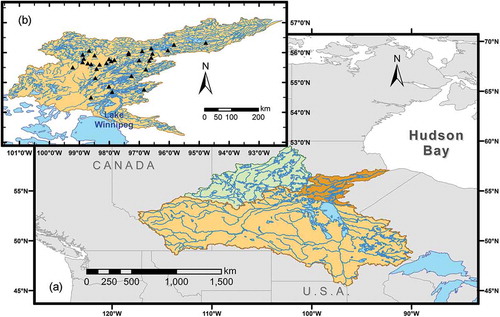
The watershed is located in the mid-latitude Canadian Boreal forest ecoregion, is wetland and surface water dominated, with a temperate climate (Köppen Climate classifications: Dfb, Dfc). Owing to hydropower operations within the basin, its largest rivers are regulated by control structure and run-of-the-river hydropower dams, while the headwaters are unregulated and undeveloped. Sporadic discontinuous permafrost (10–50%) underlays most of the basin, while the downstream northeastern portion is up to 90% permafrost. The region has extremely low relief, with a maximum elevation of 335 m a.s.l. and the outlet to Hudson Bay at sea level; the average basin slope is 0.037%. The low gradient in the region results in prevalent surface water bodies, such as small lakes and wetlands, and numerous channelized lakes in the rivers. From satellite imagery, the most common land cover is coniferous forest, with 35% of the watershed covered by coniferous forest of varying densities, bogs, fens (wetlands connected to the stream channel) and wetlands cover 26% of the region; shrub areas and open water are also common, covering 16% and 14% of the basin area, respectively (Geogratis 2011).

The LNRB has a sub-arctic continental climate, characterized by cool summers, cold winters and moderate precipitation and humidity, according to the Environment and Climate Change Canada climate normal station ID 5062922 (Table 1). For comparison, annual weather data from the Thompson Airport station (ID 5062922) located near the centre of the watershed, are provided. The study period contained both warmer, drier periods (2010/11) and cooler, wetter periods (2013/14). Further details regarding the basin, its climatology and hydrological regime are provided in Smith et al. (2015) and Holmes (2016), including an assessment of basin physiography and isotope signatures from (Welch et al. 2018).

Table 1. Climatology of the Lower Nelson River Basin based on 1981–2010 climate normal period (ID 506922) and for each year of study (Environment and Climate Change Canada, 2016).

Climate variable	Climate normal	2010	2011	2012	2013	2014
Daily average annual temperature (^oC)	11.5	–0.1	–1.9	–1.9	–3.8	–4.2
Snow-free season	May–Oct	Apr–Oct	Apr–Nov	Apr–Nov	May–Oct	May–Oct
Daily average winter temperature (^oC)	–18	–9.8	–14.5	–11.9	–17.7	–15.4
Percent average annual rainfall	65	78	84	72	73	71
Percent average snowfall	35	22	16	28	27	29
Average annual precipitation (mm)	500	624	551.3	552.4	427.4	537.8
Average annual evapotranspiration (mm)	300–550	–	–	–	–	–
Open water evaporation loss (mm)	450	–	–	–	–	–
Average annual relative humidity (%)	58–79	–	–	–	–	–

– no data; not available in daily station records.

Basin regulation

The hydrology of the Nelson-Churchill River Basin is of operational significance to Manitoba Hydro, who currently operate six hydroelectric generating stations within the LNRB, with one additional station under construction. These stations are located on the Nelson and Burntwood rivers and operate using run-of-the-river flows (i.e. without significant reservoirs). The majority of the flow in the Nelson River originates from Lake Winnipeg, with 2200 m³ s⁻¹ on average entering the LNRB from the lake, or about two-thirds of the total flow at the Nelson River outlet (Water Survey of Canada 2019). Significant flows also enter the basin via the Churchill River Diversion (CRD), which connects the Churchill River at South Indian Lake to the Rat River in the northwest LNRB (i.e. a tributary of the Burntwood River), with an average annual flow of 790 m³ s⁻¹ (1978–2014) (Manitoba Hydro 2015). Flows from the CRD are regulated by the Notigi Control Structure, which has a license maximum of 850 m³ s⁻¹ but can pass up to 990 m³ s⁻¹ under current licensed regulation (Duenas 2016). The CRD is operated based on flow demand for the downstream hydro-electric generating complex.

Data and methods

Modelling methods

An enhanced version of the original isoWATFLOOD^TM model (Stadnyk et al. 2013) was developed that includes dual-isotope simulation (δ¹⁸O and δ² H), along with explicit transpiration fluxes and continuous snowpack modelling. The coupled hydrological model used for this implementation is WATFLOOD^TM, a semi-distributed hydrological model discretized via grouped response units (GRUs) and employing both conceptual and physical process representations (Kouwen 2018). The isotopic composition of storages representing the snow, surface and upper soil zone of each hydrologically unique land/soil classification (GRU) within every grid cell, and the lower soil zone, wetland and channel storages in each cell, are continuously tracked by isoWATFLOOD^TM (Fig. 2).

Figure 2. Illustration of isoWATFLOOD^TM fluxes and storages within a grid cell (adapted from Holmes 2016). Individual boxes represent unique storage compartments associated with land cover units or river classifications.

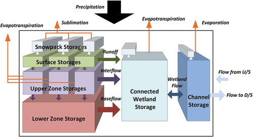
The enhanced version of isoWATFLOOD^TM includes: (1) snowpack storage accounting for time-variable precipitation composition and land cover-specific sublimation and melt rates; (2) transient surface storage mixing for rain and snowmelt isotopic inputs, which act as source waters for infiltration and overland runoff; (3) shallow soil or upper zone (UZ) storage with variable saturation and distinct fractionating (evaporation) and non-fractionating (transpiration) fluxes for each land cover; (4) lower zone (LZ) storage simulating the fully saturated zone with mixed inputs from a larger regional flow system used to source baseflow flux; (5) connected or riparian wetland storages that mix runoff (new water) and channelized water (old water), including delayed water retention and separation of transpiration and evaporation fluxes; and (6) open water and lake storages that account for ice-cover, rain and snowmelt inputs, evaporative fractionation, and inflows from adjacent storage and upstream grid cells. A summary of these modifications, and brief description of their hydrology is provided in the Supplementary material (Table S1).

Accurate simulation of isotopes at the mesoscale (>1000 km²) requires the simulation of evaporative enrichment, which produces isotopically distinct signatures of water that have undergone evaporation. In isoWATFLOOD^TM, water is fractionated from lakes, connected wetlands and near-surface (UZ) soil water; where evaporative fractionation is modelled using an adaptation of the Craig and Gordon (1965) model developed by (Gonfiantini et al. 2018). The evaporated water composition is applied to tracer mass balances for the evaporation component of the evapotranspiration loss from the soil zone. Fractionation occurring from connected wetlands and lakes is computed using the respective fraction- and time-dependent isotope balance equations presented by (Gibson 2002). The implementation for δ² H is consistent with the implementation for δ¹⁸O described in (Stadnyk et al. 2013).

Model data

As a partially physically based model, the (iso)WATFLOOD model(s) requires a wide range of input data. The LNRB setup of WATFLOOD used forced streamflow at the Nelson River at Jenpeg (05UB009) and below Sea River Falls (05UB008) along the East Channel to simulate outflow from Lake Winnipeg, and at the Notigi Control Structure along the Rat River to simulate inflow from the Churchill River system. The model extends downstream to the Nelson River estuary region near Hudson Bay. The domain is divided into 100-km² grid cells (10 km resolution) and nine distinct river classes depending on streamflow characteristics and river morphology. Grids are further subdivided into nine dominant GRUs determined from satellite-derived land cover imagery and surficial geology maps (Fulton 1995, Geogratis 2011).

Precipitation and temperature records from 13 Environment and Climate Change Canada (ECCC) weather stations in the LNRB and the surrounding region were used as climatic input (Environment and Climate Change Canada 2018); point values were distributed across the basin using distance-squared weighting (Kouwen 2018). Relative humidity was added to the model in this study for the simulation of isotopic fractionation and was derived from the six ECCC stations that had observations within the LNRB during the simulation period. Humidity observations were distributed in the same manner as air temperature data.

The isotope simulation additionally required the isotopic composition of precipitation as model forcing. Distributed precipitation compositions from the empirical model developed by Delavau et al. (2015) were used to vary precipitation composition spatially and temporally (on a monthly timestep). The model was dependent on latitude and precipitable water content, among other variables derived from reanalysis data for the c Köppen regionalization. We compare isoP simulated monthly compositions from the Delavau et al. (2015) model to observed composite isotope in precipitation samples collected during the period of study and find the modelled compositions perform satisfactorily (Supplementary material, Fig. S1). Inflows used to force the model from upstream areas used observed isotopic compositions from sampling at all three forcing locations: Jenpeg, Notigi and the Nelson River east channel. Forced inflows were assigned the most temporally proximate observed isotopic composition.

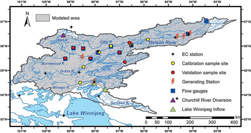
The isotope simulation was constrained to a 5-year period (2010–2014) containing isotope observations, including calibration and validation, while the hydrological simulation was run over the entire study period (1981–2014) to sufficiently establish hydrological storages and antecedent conditions. Hydrometric data in the LNRB are scarce, with 17 active streamflow gauges or an average of one gauge per 5300 km². The duration of continuous flow records varies, with the earliest commencing in 1957, and an average continuous record length of 40 years (Water Survey of Canada 201). Four flow gauges are located at the generating stations along the Nelson River controlled by the operator, Manitoba Hydro: Jenpeg, Kelsey, Kettle and Long Spruce (see Fig. 3). As flows from generating stations are regulated, these gauged records are much less useful for model calibration and validation. Hydrometric gauging stations are not equally distributed throughout the basin (Fig. 3); with higher station density in the north and northeast of the basin and zero active stations in the southwest.

Figure 3. Calibration and validation gauge locations within the LNRB, along with location of hydro-electric generating stations.

Isotopic observations extend from March 2010 to the present as part of the Stable Water Isotope Monitoring Network (SWIMN) (Smith et al. 2015). The majority of samples are taken from surface waters (rivers and lakes), with three locations where precipitation samples are taken, three shallow groundwater sample sites, and one Class A evaporation pan. Winter sampling of groundwater is not possible due to freezing and composite snow samples are taken in place of liquid precipitation collection, albeit only once per year due to the remoteness of the site. Given the difficulty with accessing the site over winter, it was not possible to monitor time-variant snowpack or snowmelt samples, including accounting for redistribution of the snowpack. Due to the model resolution (100 km²), however, it is reasonable to assume redistribution would occur internal to a single grid and not alter a grid mass balance. Redistribution among landcovers was not accounted for.

Isotope sampling occurs at most hydrometric stations where flow is measured in the LNRB and also at other sites in the central LNRB based on accessibility and hydrological significance. Surface water sampling locations are generally sampled once or twice a month during the open water season and occasionally during the ice-on period; amounting to 5–6 samples per year, on average. Additionally, a basin-wide synoptic survey was performed annually in early summer at regular gauges and additional sampling sites (2011–2016); an autumn synoptic survey was conducted once in 2015. Surface water samples were collected from turbulent flow regions using a 500-mL collector bottle attached to an extendable pole. Two 30-mL samples were filled from the collector bottle and placed in high-density polyethylene Nalgene® bottles, capped and sealed with electrical tape to minimize evaporation. During ice-on, water samples are collected by auguring through the ice cover and sampling water using a plastic bailer. Samples are analysed for deuterium and ¹⁸O at the University of Victoria Environmental Isotope Laboratory managed by Alberta Innovates Technology Futures. Isotope compositions are obtained using a Delta V Advantage stable isotope mass spectrometer; a Gasbench II peripheral was used for ¹⁸O, and an HDevice peripheral for deuterium. Results are standardized by comparing the in-house standard with Vienna Standard Mean Ocean Water (VSMOW2), isotopic compositions being reported relative to VSMOW2 as delta values (‰). The uncertainty in the reported values is ±0.2‰ for ¹⁸O and ±1‰ for ² H.

Model calibration

Following initial model set-up, a preliminary, regional calibration was performed using hydrometric data over a period of 12 years of record (2003–2011). The WATFLOOD autocalibration methodology, the dynamically dimensioned search algorithm (DDS), was used to derive this regional parameterization, which was the starting point for our study. Further details on the regional parameterization and calibration methodology and model set-up are provided in Holmes (2016).

We established two different calibration methodologies in this study to assess the value of isotopically enabled models within fully automated calibration (Method 1) and manual calibration (Method 2) approaches (Fig. 4). Whereas Method 1 focuses on achieving good streamflow performance metrics (hydrometric flow and river isotope compositions), Method 2 is designed to focus on flowpath and hydrological process functioning, for comparison.

Figure 4. Calibration methodologies applied in this study, where Method 1 performs autocalibration using DDS and three different optimization algorithms incorporating flow-only (F), oxygen-18 isotope (O) and dual-isotopes (OH); and Method 2 used manual adjustment from the original regional parameterization, informed by the dual-isotope frameworks. Long term simulation was performed on the regional parameterization and following both Method 1 and 2 calibrations, for comparison.

First, isotope error was introduced into autocalibration by coding new DDS optimization algorithms. In DDS, we conducted three separate model calibrations, resulting in three distinct parameter sets for the flow-only calibration (F), flow and ¹⁸O calibration (O) and a flow and dual-isotope (¹⁸O and ²H) calibration (OH). Calibrations were compared over a 28-year hydrological simulation period (1982–2009) to assess long-term model performance. The second method used a manual calibration, also starting from the original regional parameterization; this was performed using isotopes to verify internal modelled processes and inform manual corrections to select parameters controlling those processes. Similar to Method 1, following this manual calibration, long-term simulation was performed (1982–2009) to assess long-term model performance in comparison to Method 1 results.

Autocalibration (Method 1) was performed using an external executable for the DDS algorithm that works in conjunction with the WATFLOOD executable to run DDS, as described in Tolson and Shoemaker (2008). The DDS algorithm searches the parameter space to optimize model performance, with the distance moved within the parameter space changing as a function of the parameter limits (Table 2) and the total number of parameter sets evaluated relative to the total number of parameter sets being evaluated (10 000 in this study). The DDS method is efficient, which is important for models having large numbers of parameters, like WATFLOOD, and would therefore be capable of producing good calibration results, often while avoiding poor quality local optima (Kouwen 2018). The current implementation of DDS for WATFLOOD used in this research saved only the final parameter set and evaluated parameter set performance using a single error function; it was therefore incapable of performing uncertainty assessment.

Table 2. Parameter lower and upper limits for DDS calibration.

Parameter function	Parameter name	Lower limit	Upper limit
Lower zone coefficient (m s^−1)	flz	1.00 × 10^−8	5.00 × 10^−3
Lower zone exponent	pwr	1	4
Channel Manning’s n	r2 n	1.00 × 10^−3	2.00 × 10^−2
Wetland or bank porosity	theta	0.1	0.95
Wetland/bank lateral conductivity (m s^−1)	kcond	0.1	0.25
Melt factor (mmºC^−1 h^−1)	fm	5.00 × 10^−2	0.25
Interflow coefficient	rec	5.00 × 10^−2	4
Upper zone retention (mm)	retn, forest	20	150
Upper zone retention (mm)	retn, sparse/short veg	10	50
Upper zone retention (mm)	retn, wetland	30	400
Recharge coefficient bare ground	ak2	1.00 × 10^−3	0.2

Nash–Sutcliffe error (E_NS) was selected to assess streamflow performance, as it is well understood by modellers, frequently used and includes both flow timing and volume error in its final evaluation. Using E_NS for calibration has known limitations: a bias toward high flow periods and under-estimation of variability, such that simulated hydrographs tend to flatten relative to the observed hydrograph (Kunstmann et al. 2006, Gupta et al. 2009).

(1) $E_{\mathrm{N}\mathrm{S}}=1-\frac{{\sum }_{i=1}^n{\left(Q_s-Q_i\right)}^2}{{\sum }_{i=1}^n{\left(Q_i-Q_i^{\ast }\right)}^2}=1-\frac{E_{\mathrm{M}\mathrm{S}}}{{\sigma }_o^2}$(1)

where $Q_S$ is the simulated streamflow (m³ s⁻¹) in a given timestep, $Q_S$ is the observed streamflow (m³ s⁻¹) in the same timestep, $Q_i^{\ast }$ is the mean streamflow at the gauging point, E_MS is the mean square error of streamflow, and ${\sigma }_o^2$ is the variance of the observed discharge.

Though E_NS could also be used for isotope error, it was deemed unsuitable for application to the LNRB isotope dataset given the observations at many sites were taken both rarely and irregularly. As E_NS is normalized using observed variability, and irregular sampled sites would tend to have under-sampled variability, applying this statistic would introduce weighting problems when averaging errors across multiple sites with differing sampling regularity. Instead, we selected normalized root mean squared error (E_NRMS) to assess the isotope simulation error, defined as:

(2) $E_{NRMS}=\frac{\sqrt{{\sum }_{i=1}^n{\left(I_o^i-I_s^i\right)}^2}}{\left|\overline{I_o}\right|}$(2)

where I_o is the observed isotopic composition (per mille, or 10⁻³) and I_s (per mille, or 10⁻³) is the simulated isotopic composition in any given timestep. Since it is normalized by the mean isotopic composition, $\left|\overline{I_o}\right|$ (per mille, or 10⁻³), rather than the variability, the E_NRMS is much less sensitive to the number of observations at a site when compared to E_NS. We choose the E_NRMS function because of its relative weight in considering error resulting from both timing and volume. The error function used by the DDS-WATFLOOD executable is user-specified, with the only requirement being that it produces a single error value.

We tested three distinct error functions to compare traditional flow-only calibration to coupled flow-isotope calibration. The first used only flow error (F) and was simply the average E_NS across calibrated streamflow gauges, which was an existing metric commonly used by the DDS-WATFLOOD executable. Two new error functions were added to incorporate isotope data: one including flow and ¹⁸O observations (O), the second utilizing flow and both simulated isotopes (¹⁸O and ²H, OH). The first error metric utilized average E_NS for flow error and E_NRMS for ¹⁸O error, with the two components equally weighted. The dual-isotope error function similarly used average E_NS for flow error, and the average E_NRMS of both ¹⁸O and ²H error, again with components equally weighted. All sites having flow and isotope data were equally weighted in the evaluation, and a total of 10 000 simulations were run for each of the three model calibrations (F, O and OH). The three error functions resulted in three distinct (and comparable) parameter sets: the flow calibration set (F), the flow and ¹⁸O calibration set (O) and the flow, ¹⁸O and ²H calibration set (OH).

As a distributed hydrological model, WATFLOOD has 24 parameter types potentially available for inclusion in the autocalibration process. As each river and land class has its unique parameter values, the total number of parameters included in the calibration could be extremely large. To restrict the number of calibrated parameters without negatively impacting final performance, only parameters having substantial impact on either the flow or isotope simulations without alternate means of parameter value selection were included in autocalibration. A sensitivity analysis performed prior to model calibration determined the parameters to be included in calibration (Holmes 2016). Nine parameter types met these criteria, resulting in a total of 72 calibrated parameters once multiplied across landcover classifications and river types. Table 2 summarizes the nine parameter types selected, where upper zone retention (retn) was included for three specific land classifications.

An independent manual calibration was also performed, where parameter values were selected individually and sequentially to optimize the agreement between dual-isotope simulations and observations for hydrological storages using the isotope framework (Method 2). The isotope-verified parameter selection began with soil water parameters, followed by baseflow, wetland and river channel parameters.

A 5-year calibration period (2010–2014) was used for all calibrations, with 2009 used for model spin-up. This period was selected for two reasons: it coincides with the period of isotopic observation in the LNRB, and it contains a range of hydrological conditions (wet and dry) allowing for more robust flow and isotopic calibration. Ten streamflow gauges and six isotope sampling sites (see Fig. 3) were used for the autocalibration, with calibration sites distributed as uniformly as possible across the basin given the limited number of gauges (Table 3). Streamflow simulations were validated using a split-sample in time approach from 1982–2009, or the period of record available for each of the 10 hydrometric gauge locations. Isotopic simulation was validated at seven isotope sampling sites not used in the calibration (see Fig. 3). If flow data were not available for the entire validation period, validation was conducted on the period of record available, beginning in 1982 or the start year of record (Table 3).

Table 3. Calibration (2010–2014) and validation hydrometric gauge summary for streamflow simulation.

Water Survey of Canada Gauge Name	Gauge ID	Drainage area(km^2)	Start year*	Mean annual discharge(m^3 s^−1)
Burntwood River above Leaf Rapids	05TE002	5 810	1985	22.9
Footprint River above Footprint Lake	05TF002	643	1977	3.21
Sapochi River near Nelson House	05TG006	391	1992	2.15
Odei River near Thompson	05TG003	6 110	1979	34.3
Burntwood River near Thompson	05TG001	18 500	1957	621
Taylor River near Thompson	05TG002	886	1970	5.07
Grass River above Standing Stone Falls	05TD001	15 400	1959	64.6
Nelson River at Kelsey Generating Station	05UE005	1 050 000	1960	2 300
Weir River above the mouth	05UH002	2 190	1977	15.6
Limestone River near Bird	05UG001	3 270	1976	21.5

*Validation period starts in 1982, or start year of the hydrometric record, and was run continuously until the end of 2009.

It is important to note that isotope calibration and validation sites did not always overlap with hydrometric gauging sites (streamflow calibration/validation sites) since our isotope monitoring network included many more locations than the hydrometric network (Smith et al. 2015); the longest and most complete isotope sampling sites were selected for model calibration and validation. A long-term simulation was also run using the original, regional parameterization for comparison against Method 1 and Method 2 validations.

For model evaluation, the deviation of runoff volume error, D_v, was also computed to assess the model performance in terms of predicted volume of water in storage:

(3) $D_v=\frac{{\sum }_{i=1}^N\left(Q_s-Q_i\right)}{{\sum }_{i=1}^N{Q}_i}\times 100$(3)

where Q_s (m³ s⁻¹) is the simulated streamflow or storage volume (mm) in any given timestep, Q_i (m³ s⁻¹) is the observed streamflow or storage volume (mm) and N is the total number of values within the period of analysis. The D_v performance metric is reported in percent, with a value of 0 indicating an exact match between simulated and observed volumetric flow or storage over the period of analysis.

Results and discussion

DDS calibration

The three resulting parameter sets all produced acceptable simulations, based on relevant literature (Moriasi et al. 2007, 2015), at all streamflow gauges included in the autocalibration (Table 4). Streamflow simulation statistics are equivalent across all three calibrations, with no statistically significant difference when including isotopes in the DDS autocalibration. The use of isotope simulation error in the objective function is associated with a small decrease in E_NS values and a slight improvement in the flow volume error, but changes are too small to be statistically significant given the number of sites included in the calibration.

Table 4. Streamflow performance evaluated by parameter sets derived using three different objective function definitions in DDS incorporating flow-only (F), flow and oxygen-18 (O) and flow and dual isotope (OH) into model calibration. The p values are provided in brackets for O and OH simulations relative to flow-only calibrations (F).

	Calibration (2010–2014)			Validation (1982–2009)
Metric	F	O	OH	F	O	OH
ENS	0.670	0.664 (0.92)	0.663 (0.91)	0.629	0.619 (0.88)	0.622 (0.92)
Dv (%)	–2.92	–1.93 (0.91)	–1.66 (0.89)	–8.63	–7.23 (0.90)	–6.91(0.87)
ENRMS O	0.063	0.053 (0.59)	0.054 (0.67)	0.111	0.134 (0.65)	0.130 (0.72)
ENRMS H	0.049	0.051 (0.87)	0.043 (0.69)	0.083	0.086 (0.89)	0.083 (1.0)

Likewise, flow statistics are insignificantly different during model validation. The E_NS values similarly decreased, albeit not significantly, and there were generally smaller volume errors. Results indicate that incorporation of E_NRMS from isotope simulation into a single-objective autocalibration neither aided nor impeded calibration of the hydrological model. Though this is not evidence that isotope-enabled calibration has improved model calibration, this result is significant in that it highlights that the addition of another constraint during model calibration has not, in fact, degraded model performance during the calibration period. It is encouraging that a statistically equivalent calibration can be reached even when imposing additional constraints on the model, using the isotope observations.

Long-term simulation performance

Though streamflow values were generally well simulated during the validation period (1982–2009), substantial variation in performance was found between the calibration and validation periods. Gauges with marginal simulation statistics during calibration showed good performance in validation; however, several gauges with good or very good calibrations performed poorly during validation. The lack of predictability of model performance during validation is a non-trivial problem given one of the primary applications of hydrological models is to simulate flows outside periods of record. The prediction of long-term model performance from calibrated E_NS as a single model performance indicator was found to be unreliable (Fig. 5(a)), with only a weak, statistically insignificant correlation (R² = 0.25, p = 0.2) between E_NS calibration and validation scores. The other flow simulation statistics proved even less reliable at predicting model validation performance.

Figure 5. Long-term simulation (1982–2009) performance relative to short-term calibration (2010–2014) for flow using (a) E_NS for flow-only calibration (F), (b) isotope E_NRMS for oxygen-18 calibration (O), (c) dual-isotope E_NRMS for both isotopes (OH); and (d) both single (x-axis) and dual-isotope (y-axis) simulation errors (E_NRMS) plotted against each other over the calibration period.

Isotope simulation error from the 5-year calibration period (E_NRMS, 2010–2014), on the other hand, is capable of reliably predicting streamflow E_NS from the validation period (R² = 0.85) (Fig. 5(b)). Using a single-isotope error metric (e.g. from ¹⁸O simulation) is equivalent to dual-isotope simulation in terms of predictive capability, with only a small decrease in the R² value to 0.82 (p = 0.008 for flow-only calibration). The two isotope errors are not interchangeable, though deuterium (y-axis) is still a statistically significant predictor of flow performance with R² of 0.65 (p = 0.02) for flow-only calibration when compared to ¹⁸O error (x-axis) (Fig. 5(d)). If single-isotope simulation is used, ¹⁸O is more useful, likely due to the higher relative magnitude of evaporative fractionation effects.

Although isotope-flow calibrations do not perform any better than the flow-only calibrations during the validation period (statistically no difference), the predictive capability of isotope simulation error demonstrates that isotope-enabled simulation does have the potential to improve calibration. An alternate method of incorporating isotope data in autocalibration could possibly produce better performing long-term simulations, though would likely not result in better calibration performance. Isotope-enabled calibration should not be expected to outperform flow-only calibration for the simple fact that simulations are now forced to meet two (or more) criteria during optimization, rather than a single-objective criterion for streamflow. This study highlights that this does not, however, mean that isotopes have not improved the model calibration, which can be witnessed by model performance during validation. In place of the single-objective function used in this study, isotope error could be evaluated in one objective using a multi-objective calibration methodology, or isotope error might be used as a model constraint (i.e. used to limit the simulation) rather than as an optimization objective.

Internal process verification using isotopes

Given that isoWATFLOOD^TM simulates ¹⁸O and deuterium isotope compositions for not only streamflow but also all internal storages and fluxes numerically computed in the WATFLOOD model, internal process verification is possible using observed isotope data, where it exists. Simulated internal process compositions can be compared to observed isotopic compositions of significant hydrological storages (e.g. groundwater or wetland storages) to verify internal flowpaths and storage compositions derived during model simulation. Such verification is theoretically possible using observed water volumes and flows, but in practice (and particularly in remote, mid- to high-latitude basins), obtaining these observations is either prohibitively expensive (e.g. measuring groundwater), or technically infeasible (e.g. measuring volumes and flows in large wetlands with numerous inflow and outflow channels). Stable isotope sampling is simpler, less laborious and time-consuming; and although groundwater sampling still requires drilling, only occasional monitoring is needed. Adequate isotope data for model verification are cheaper to acquire and observe using periodic grab samples, which are sufficient for providing information on longer-term processes. Since the isotope monitoring network in the LNRB included shallow groundwater and wetlands, as well as streams and lakes, this provided an opportunity to assess processes internal to the model, and therefore constraints on parameter values tied to those processes; essentially opening the proverbial black-box of hydrological modelling (Juston et al. 2013). As with streamflow sampling, source water sampling in the LNRB was both sparse and irregular which precluded a quantifiable analysis with statistical certainty but was frequent enough to warrant an assessment of the potential utility of isotopic data for parameter value selection in calibration.

Evaporation is most clearly distinguished using stable isotopes in water, whether observed or simulated. Given isotope composition is most responsive to changes in evaporative fractionation, the evaporative loss simulated by WATFLOOD can be validated by comparing simulated isotope frameworks (δ¹⁸O-δ²H space) to observed data collected in the LNRB sampling program (Fig. 4, Method 2). Due to the continuous nature of simulated isotope compositions (i.e. hourly timestep over 5 years), individual simulated points are used to derive best-fit lines, or local mixing lines, for specific storages on the simulated framework. Since compositions are for storages (not fluxes), values are not flux-weighted except in the case of precipitation and evaporation. We demonstrate the output from a three-stage manual calibration process that, instead of requiring best fit streamflow performance, required only best fit dual-isotope framework local mixing line (LML) slopes for internal simulated storages. [Incremental parameter adjustments for each stage (storage component) are provided in the Supplementary Material (Table S2), along with calibration results for LML slopes (Table S3) that correspond to Fig. S2 best-fit results.] Results are shown for the Odei River Basin (and its tributaries) because manual calibration and isotope verification (Method 2) was focused on this region due to adequate isotope data availability (temporal resolution of sampling, and process-based sample availability).

Observed shallow groundwater values generally follow the meteoric water line (LMWL) in the LNRB, with some groundwater samples showing moderate enrichment, i.e. diverging from the LMWL and toward the slope of the local evaporation line (LEL). Observations therefore indicate that, for the LNRB, shallow groundwater, or soil water, is primarily mixed precipitation that is only moderately subjected to evaporative losses (Fig. 6).

Figure 6. Simulated isotope framework (2010–2014) from isoWATFLOOD^TM indicating best-fit lines for soil (purple) and groundwater (red) storages relative to observed isotopic values (black dots) from shallow piezometers. Grey lines represent isotope framework components derived from long-term observed data for the LNRB derived by Smith et al. (2015).

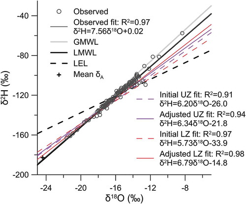
Post-calibration, the initial upper zone retention parameter (i.e. retn = 120 mm) controlling evapotranspiration rates in WATFLOOD produces large and persistent changes in isotopic composition from (fractionating) evaporation in the upper zone. This parameter value was originally optimized across all sub-basins with similar vegetative cover during the autocalibration process but does not produce satisfactory isotope simulations based on observed soil water compositions. Only the lower range of possible parameter values for this retention parameter are found to produce simulations in agreement with observed soil water isotope slopes on the framework. Therefore, from this analysis, we could conclude that the parameter range used in autocalibration should be reduced to 20–60 mm, from the 20–150 mm standard range reported in the WATFLOOD manual (Kouwen 2018). This is useful information during autocalibration as it narrows the effective parameter space, enabling the model to focus on a smaller search radius and potentially converge quicker on better solutions (Razavi et al. 2019).

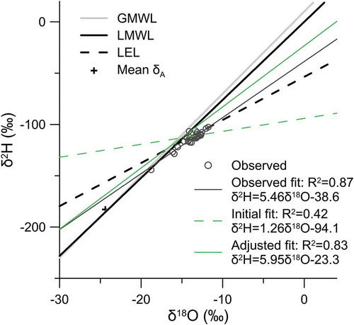
In WATFLOOD, water moves from the upper zone to the connected wetlands through the interflow flux component. The wetland storage compartment is also subjected to an evaporative loss flux. Evaporation from the connected wetland is largely controlled by the porosity parameter (i.e. theta), which determines the wetland storage depth and hence water available in storage for evaporation to occur. The local mixing line (LML) derived from the observed wetland isotope samples (grey line) falls between the LMWL and LEL (Fig. 7), while the simulated wetland mixing line (dashed green line) from the autocalibration-derived wetland theta parameter that has a higher slope that is closer to that of the LMWL. Increasing the theta parameter effectively increases evaporative losses from wetland storage, resulting in a recalibrated wetland mixing line (solid green line) that is in better agreement with observed compositions. In the case of the LNRB, theta values over 0.6 produce isotopic simulations closer to observed compositions, and the original theta value of 0.4 is therefore found to be too low. The parameter value lower limit used in autocalibration could therefore be increased from 0.1 to 0.6 for the LNRB to further constrain the model parameter space.

Figure 7. Simulated isotopic framework (2010–2014) from isoWATFLOOD^TM indicating best-fit lines for wetland (green) storage relative to observed isotopic values (grey circles) sampled from open water wetlands. Grey lines represent isotope framework components derived from long-term observed data for the LNRB, and the black line indicates the flux-weighted LMWL derived by Smith et al. (2015).

Using the dual-isotope simulation to assess simulated evaporation losses in comparison to observed isotopic compositions of hydrological storages has resulted in the reduction in plausible parameter value ranges for multiple hydrologically significant parameters. By reducing the number parameter search space during the calibration process, isotope-enabled simulation has potentially improved the efficiency of calibration, in addition to improving the physical basis of the parameter values. Supplementary Material Fig. S2 demonstrates that by adjusting internal simulated processes, the resulting streamflow isotopic values improve relative to observed river isotope data (here, initial fits correspond to those derived from the regional parameterization).

Despite these benefits, adjusting parameters post-calibration can result in degrading streamflow performance, which is often undesirable for modellers. Table 5 summarizes the incremental change in streamflow performance statistics associated with the isotope-informed parameter adjustments (Figs. 6 and 7) for long-term simulations using daily averaged annual hydrographs relative to observed streamflow (Fig. 8(c)).

Table 5. Incremental change in streamflow simulation performance statistics associated with isotope-informed parameter adjustments (Fig. 4, Method 2).

	ENS	Dv	R^2
Regional parameters (2010–2014)	0.63	–19.5	0.67
Calibrated (2010–2014)	0.67	–3.4	0.68
Validation (1982–2009) Regional parameters	0.69	–19.3	0.73
Isotope verified	0.69	–1.78	0.70

Figure 8. Post-calibration daily averaged (a) isograph, (b) hydrograph and (c) average annual hydrographs (1982–2009) for Method 1 flow-only (F), single-isotope (O) and dual-isotope (OH) calibrations, relative to Method 2 (Fig. 4) manually adjusted (IV: isotope verified) using dual-isotope framework. For reference, the long-term simulation from the regional parameterization (R: regional simulated flow) is included, and the observed discharge (solid black line). Solid black dots are observed isotopes.

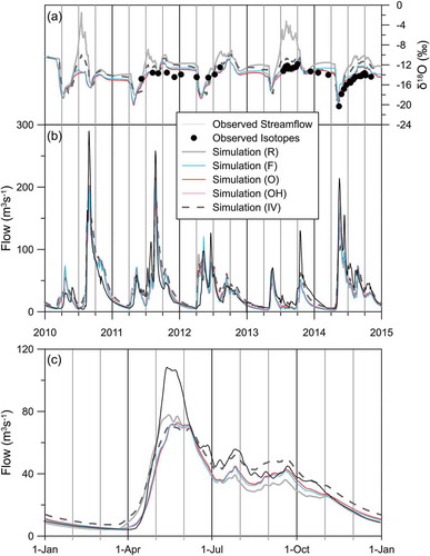
There are statistically insignificant changes in streamflow resulting from the choice of calibration method (flow-only, single and dual-isotope) in all metrics except volume deviation (D_v). This is revealing considering the differences in long-term model performance reported in Fig. 5 and demonstrates that satisfactory model performance during a relatively short calibration period using streamflow metrics can yield misguided confidence in models being used for long-term analysis, particularly under non-stationary climates. When the model calibration is manually adjusted using feedback from the dual-isotope framework analysis (Fig. 4, IV-Isotope Verified parameters), a statistically significant change in calibrated streamflow is observed (Fig. 8), which is reflected in the validation (isotope verified) results in Table 5 through a significant improvement in volume-based simulation. Though direct verification of parameter values is not possible here, isotope data did provide additional constraint on the possible range of parameter values through the imposed, additional requirement to match observed isotope data. Our results show the dual-isotope approach yields similar, if not improved (volume) model performance, and demonstrates the additional information content provided to modelers that is otherwise not available via hydrometric calibration alone.

Figure 8(c) demonstrates that the isotope verified (IV) simulation is most beneficial in improving simulated late summer and fall streamflow relative to the other calibrations. Water isotopes are particularly good tracers of evaporation and our results highlight the value of improving summer and autumn hydrological storages within lakes and wetlands for the accurate prediction of seasonal runoff. This is in line with the work of Gibson et al. (2017), who showed that isotope-based methods are effective at constraining lake and wetland evaporation loss across the Boreal Shield environment, which aid in estimation of water yield, or regional runoff.

The IV simulation also better estimates the timing of the spring freshet based on the slope of the rising limb from the average annual hydrograph (Fig. 8(c)). This is likely attributable to the improvements in late summer and fall antecedent storage and baseflow recession (Fig. 8(b)) in the season preceding freeze-up and the subsequent melt period. The accurate prediction of peak runoff volume and timing is highly dependent on pre-freeze-up storage initialization (Unduche et al. 2018), which the IV simulation is better able to capture by constraining the isotopic enrichment (Fig. 8(a)).

An important aspect for coupled hydrologic–isotope approaches is evapotranspiration (ET) partitioning. Jasechko et al. (2013) demonstrate that up to 80% of water loss from terrestrial, Boreal ecosystems globally can be attributed to transpiration, which is considered non-fractionating. Here, we can see that none of the models accurately capture the magnitude of summer isotopic composition (Fig. 8(a)). Welch et al. (2018) state that wetland-derived evaporative enrichment was significant in this region and had a direct impact on riverine isotopic compositions. Smith et al. (2018) similarly emphasized the importance of considering seasonally varying ET partitions in Boreal regions for the accurate estimation of riverine compositions in wetland-dominated landscapes. From Fig. 8(c) it can be seen that late autumn streamflow is generally overestimated by the IV simulation, which is suggestive of an underestimation of hydrological loss (from open water and wetlands), relative to the other calibration methods, perhaps triggered by an overestimation of the E/ET partition.

It is noted that none of the calibrated models do a good job of accurately simulating peak flow volume. This is likely attributable, in part, to the statistics chosen for the model calibration, which deliberately put less emphasis on annual peak flow estimation. The introduction and weighting of isotope volume error in autocalibration means there is a trade-off between the model’s ability to simulate annual peak flow versus long-term storage (Moriasi et al. 2015). It should be noted that the IV simulation was conducted independent of flow optimization and did not explicitly consider streamflow fit (instead focusing on isotope simulation). Lastly, in this study, the model calibration period was relatively short in comparison to traditional model calibration recommendations (Moriasi et al. 2015) and was limited by isotope record length. It is preferred that a calibration period of 10 years or so be used to capture inter-annual variability in runoff generation mechanisms. By limiting the calibration period, we generate a less robust model that is incapable of accurately simulating peak flow over the long-term record. For comparison, we can observe that the peak flows during the calibration period (2010–2014) are much better simulated than over the long-term record (Fig. 8(b) and (c)).

Although Fig. 8 demonstrates the benefit of considering isotopes within the model calibration process, improvements can be made. Manual calibration with isotopes, though reasonably effective in this study, is not feasible across large spatial and time scales. Moreover, we can see significantly inter-annual variability in the IV simulation performance (Fig. 8(b)). By incorporating isotopes into autocalibration (O and OH), we see improvement over the flow-only (F) simulation by the model. This study presents the first attempt at incorporating isotopes into autocalibration, with perhaps more gains to be made if isotopes were incorporated in a more sophisticated multi-objective optimization, such as Pareto-front analysis (Asadzadeh et al. 2014). Multi-objective optimization methods would enable modellers to make more informed decisions regarding the trade-off between more accurate storage-based estimation (using isotopes) and streamflow simulation (hydrometrics).

Conclusions

Using isotope simulation error in the optimization function did not clearly improve the calibration of the model (as measured by traditional efficacy criteria), but this does not mean that isotopes were not beneficial to model calibration. Model performance did not degrade with the addition of isotope data; a statistically equivalent flow simulation was obtained despite imposing additional constraints on the model calibration exercise. Moreover, the calibration benefited from the simulation of isotopes as isotope error was found to be the best predictor of streamflow simulation performance beyond the calibration period, with ¹⁸O providing a more informative metric than deuterium. Adequate isotope data for model validation would in fact be cheaper to acquire and observe using periodic grab samples, which are enough to provide information on longer-term processes.

Alternative methods to include isotope error in the calibration should be explored as the method tested in this study had only minor effects on the calibrated parameter set. Isotope error could be included as one objective in a multi-objective calibration methodology. The potential for isotope simulations to reduce equifinality in hydrological models should be investigated to determine if adding isotope simulation error reduces equifinality, and if so, by what degree. A large number of parameter sets can be generated using a Monte Carlo type method, and the number of behavioural models compared when only flow error is considered versus when both flow and isotope error are considered. The computational cost and most efficient and effective methods of incorporating isotope error have yet to be explored.

Though source water sampling in the LNRB was both sparse and irregular, which precluded a quantifiable analysis with statistical certainty, it was found to be frequent enough to provide an assessment of the potential utility of isotopic data for parameter value selection in calibration. The isotope data provided an alternative means to narrow the range of parameter values considered during calibration, effectively reducing the parameter space and parameter uncertainty range. By reducing the size of the parameter search space during calibration, isotope-enabled simulation has potentially improved the efficiency of calibration, in addition to improving the physical basis of the parameter values; though further study is needed to quantitatively demonstrate such improvements.

The dual-isotope simulation also allowed for verification of internal hydrological flux and storage processes, which resulted in more constrained parameter ranges and resulting values than would otherwise have been possible using streamflow alone. Though this study leaves little question that parameter changes, when considering (or not) isotope data, occurred, it was limited in the number of calibration trials and therefore subject to uncertainty. Further study, with additional calibration trials, is needed to quantitatively determine the shift in internal distribution (due to model parameterization) that occurs when considering isotope error in model calibration. Adding the δ² H simulation allowed direct verification of evaporation in the model using the dual-isotope framework approach, which supports the use of dual-isotope simulation for verification and parameter identification purposes.

Although this is a first attempt at showing the value-added by isotope simulation for model calibration, this study leaves little doubt that isotope-enabled model calibration (1) does not degrade model performance, (2) improves model long-term performance, and (3) provides added-value and information content on internal model processes that is otherwise not available from hydrometric calibration alone. These aspects alone show that traditional hydrometric-only calibration is likely inadequate for long-term simulation of hydrology under non-stationary climates, and further emphasizes the need to invest in supplementary data networks to support hydrological simulation.

Acknowledgements

The authors thank the Natural Sciences and Engineering Research Council (NSERC) for their funding contributions to this research through the Discovery Grants and Postgraduate Scholarships Programs. We acknowledge the contributions of Dr Chani Welch in assisting with the initial development and scope of this work, and Dr Masoud Asadzadeh for his input on model calibration. The authors also thank the reviewers for their time providing suggestions to improve this manuscript. We acknowledge Environment and Climate Change Canada for observed streamflow and meteorological data, and Manitoba Hydro for funding and supporting the collection of isotope data used in this study. The authors declare no conflict of interest with this research and funding agencies.

Disclosure statement

This is to acknowledge that there are no financial interest or benefit that has arisen from this research, or the direct applications of this research by either author.

Supplementary material

Supplemental data for this article can be accessed here.

Additional information

Funding

This research was funded by Natural Sciences and Engineering Research Council (NSERC), under the Collaborative Research and Development Grant CRDJ-462584-13, with support from industry [Manitoba Hydro, Grant No. G277C].

References

- Asadzadeh, M.A., Tolson, B.A., and Burn, D.H., 2014. A new selection metric for multiobjective hydrologic model calibration. Water Resources Research, 50 (9), 7082–7099. doi:10.1002/2013WR014970
- Bansah, S. and Ali, G., 2017. Evaluating the effects of tracer choice and end-member definitions on hydrograph separation results across nested, seasonally cold watersheds. Water Resources Research, 53 (11), 8851–8871. doi:10.1002/2016WR020252
- Birkel, C., et al., 2016. Hydroclimatic controls on non-stationary stream water ages in humid tropical catchments. Journal of Hydrology, 542, 231–240. doi:10.1016/j.jhydrol.2016.09.006
- Birks, S.J. and Gibson, J.J., 2009. Isotope hydrology research in Canada, 2003–2007. Canadian Water Resources Journal, 34 (2), 163–176. doi:10.4296/cwrj3402163
- Coulibaly, P., et al., 2012. Evaluation of Canadian national hydrometric network density based on WMO 2008 standards. Canadian Water Resources Journal, 38 (2), 159–167. doi:10.1080/07011784.2013.787181
- Craig, H., and Gordon, L. I., 1965. Deuterium and oxygen 18 variations in the ocean and the marine atmosphere. In: E. Tongiorgi, ed. Stable isotopes in oceanographic studies and paleotemperatures. Spoleto: CNRLGN, 9–130.
- Delavau, C., et al., 2015. North American precipitation isotope (δ18O) zones revealed in time series modeling across Canada and northern United States. Water Resources Research, 51 (2), 1284–1299. doi:10.1002/2014WR015687
- Duenas, M.J., 2016. Water power act licences 2015 annual water levels and flows report. Available from: https://www.gov.mb.ca/waterstewardship/licensing/pdf/2015_awlfr.pdf [Accessed Sept 2019].
- Environment and Climate Change Canada. 2018. Historical climate data. Available from: https://climate.weather.gc.ca/index_e.html [Accessed 20 April 2020].
- Fulton, R.J., 1995. Surficial materials of Canada. Ottawa: Natural Resources Canada.
- Geogratis, 2011. Natural resources Canada. Available from: http://www.geogratis.ca [Accessed Jan 2020].
- Gibson, J.J., 2002. Short-term evaporation and water budget comparisons in shallow Arctic lakes using non-steady isotope mass balance. Journal of Hydrology, 264 (1–4), 242–261. doi:10.1016/S0022-1694(02)00091-4
- Gibson, J.J., Birks, S.J., and Moncur, M., 2019. Mapping water yield distribution across the South Athabasca Oil Sands (SAOS) area: baseline surveys applying isotope mass balance of lakes. Journal of Hydrology: Regional Studies, 21 (Dec 2018), 1–13.
- Gibson, J.J., Birks, S.J., and Yi, Y., 2017. Regional trends in evaporation loss and water yield based on stable isotope mass balance of lakes: the Ontario Precambrian shield surveys. Journal of Hydrology, 544, 500–510. doi:10.1016/j.jhydrol.2016.11.016
- Gonfiantini, R., et al., 2018. A unified Craig-Gordon isotope model of stable hydrogen and oxygen isotope fractionation during fresh or saltwater evaporation. Geochimica et Cosmochimica Acta, 235, 224–236. doi:10.1016/j.gca.2018.05.020
- Gupta, H.V., et al., 2009. Decomposition of the mean squared error and NSE performance criteria: implications for improving hydrological modelling. Journal of Hydrology, 377 (1–2), 80–91. doi:10.1016/j.jhydrol.2009.08.003
- Holmes, T., 2016. Assessing the value of stable water isotopes in hydrologic modeling: A dual-isotope approach. Thesis (MSc). University of Manitoba. Available from: http://hdl.handle.net/1993/31724 [Accessed Jan 2020].
- Holmes, T., Kim, S.-J., and Stadnyk, T., Submitted. On the implications of incorporating isotopes in multi-objective hydrologic calibration. Water Resources Research.
- Jasechko, S., et al., 2013. Terrestrial water fluxes dominated by transpiration. Nature, 496 (7445), 347–350. doi:10.1038/nature11983
- Juston, J.M., et al., 2013. Smiling in the rain: seven reasons to be positive about uncertainty in hydrological modelling. Hydrological Processes, 27 (7), 1117–1122. doi:10.1002/hyp.9625
- Kirchner, J.W., 2006. Getting the right answers for the right reasons: linking measurements, analyses, and models to advance the science of hydrology. Water Resources Research, 42 (3), 1–5. doi:10.1029/2005WR004362
- Kouwen, N., 2018. WATFLOOD/WATROUTE hydrological model routing & flood foresting system. Available from: www.watflood.ca [Accessed Jan 2020].
- Kunstmann, H., Krause, J., and Mayr, S., 2006. Inverse distributed hydrological modelling of Alpine catchments. Hydrology and Earth System Sciences, 10 (3), 395–412. doi:10.5194/hess-10-395-2006
- Manitoba Hydro, 2015. An assessment of the hydraulic impacts of the Churchill River diversion on the rat and Burntwood Rivers, PPD-15/10. Water Resources Engineering Power Planning Division, Manitoba Hydro. Available from: https://www.hydro.mb.ca/docs/regulatory_affairs/pdf/rcea/rcea_phase2_part_iv_physical_env_appendix_4_3c.pdf [Accessed Jan 2020].
- Moriasi, D.N., et al., 2007. Model Evaluation Guidelines for systematicquantification of accuracy in watershed simulations. Transactions of the ASABE, 50 (3), 885–900.
- Moriasi, D.N., et al., 2015. Hydrologic and water quality models: performance measures and evaluation criteria. Transactions of the ASABE, 58 (6), 1763–1785.
- Razavi, S., et al., 2019. VARS-TOOL: A toolbox for comprehensive, efficient, and robust sensitivity and uncertainty analysis. Environmental Modelling and Software, 112 (Oct 2018), 95–107. doi:10.1016/j.envsoft.2018.10.005
- Singh, V.P., 2018. Hydrologic modeling: progress and future directions. Geoscience Letters, 5 (1). doi:10.1186/s40562-018-0113-z
- Smith, A., Delavau, C., and Stadnyk, T., 2015. Identification of geographical influences and flow regime characteristics using regional water isotope surveys in the lower Nelson River, Canada. Canadian Water Resources Journal, 40 (1), 23–35. doi:10.1080/07011784.2014.985512
- Smith, A., Welch, C., and Stadnyk, T., 2016. Assessment of a lumped coupled flow-isotope model in data scarce Boreal catchments. Hydrological Processes, 30 (21), 3871–3884. doi:10.1002/hyp.10835
- Smith, A.A., Welch, C., and Stadnyk, T.A., 2018. Assessing the seasonality and uncertainty in evapotranspiration partitioning using a tracer-aided model. Journal of Hydrology, 560, 595–613. doi:10.1016/j.jhydrol.2018.03.036
- Stadnyk, T.A., et al., 2013. Towards hydrological model calibration and validation: simulation of stable water isotopes using the isoWATFLOOD model. Hydrological Processes, 27 (25), 3791–3810. doi:10.1002/hyp.9695
- Stadnyk, T.A., Gibson, J.J., and Longstaffe, F.J., 2014. Basin-scale assessment of operational base flow separation methods. Journal of Hydrologic Engineering, 20 (5). doi:10.1061/(ASCE)HE.1943-5584.0001089
- Tetzlaff, D., et al., 2015. Tracer-based assessment of flow paths, storage and runoff generation in northern catchments: A review. Hydrological Processes, 29 (16), 3475–3490. doi:10.1002/hyp.10412
- Tolson, B.A. and Shoemaker, C.A., 2008. Efficient prediction uncertainty approximation in the calibration of environmental simulation models. Water Resources Research, 44 (4), 1–19. doi:10.1029/2007WR005869
- Tunaley, C., et al., 2017. Using high-resolution isotope data and alternative calibration strategies for a tracer-aided runoff model in a nested catchment. Hydrological Processes, 31 (22), 3962–3978. doi:10.1002/hyp.11313
- Unduche, F., et al., 2018. Evaluation of four hydrological models for operational flood forecasting in a Canadian Prairie watershed. Hydrological Sciences Journal, 63 (8), 1133–1149. doi:10.1080/02626667.2018.1474219
- Water Survey of Canada, 2019. Water level and flow. Available from: https://wateroffice.ec.gc.ca/index_e.html [Accessed December 2016].
- Wei, Z., et al., 2019. A global database of water vapor isotopes measured with high temporal resolution infrared laser spectroscopy. Scientific Data, 6 (Jun 2018), 1–15. doi:10.1038/sdata.2018.302
- Welch, C., Smith, A.A., and Stadnyk, T.A., 2018. Linking physiography and evaporation using the isotopic composition of river water in 16 Canadian boreal catchments. Hydrological Processes, 32 (2), 170–184. doi:10.1002/hyp.11396
- West, J.B., et al., eds., 2010. Isoscapes: understanding movement, pattern, and process on earth through isotope mapping. Springer Science. doi:10.1007/978-90-481-3354-3_18