Comparative analysis of scalar upper tail indicators

ABSTRACT

Different upper tail indicators exist to characterize heavy tail phenomena, but no comparative study has been carried out so far. We evaluate the shape parameter (GEV), obesity index, Gini index and upper tail ratio (UTR) against a novel benchmark of tail heaviness – the surprise factor. Sensitivity analyses to sample size and changes in scale-to-location ratio are carried out in bootstrap experiments. The UTR replicates the surprise factor best but is most uncertain and only comparable between records of similar length. For samples with symmetric Lorenz curves, shape parameter, obesity and Gini indices provide consistent indications. For asymmetric Lorenz curves, however, the first two tend to overestimate, whereas Gini index tends to underestimate tail heaviness. We suggest the use of a combination of shape parameter, obesity and Gini index to characterize tail heaviness. These indicators should be supported with calculation of the Lorenz asymmetry coefficients and interpreted with caution.

KEYWORDS:

• upper tail behaviour
• heavy-tailed distributions
• extremes
• diagnostics
• surprise

Editor A. Fiori Associate editor E. Volpi

1 Introduction

Heavy tail phenomena have been discussed in various branches of science reaching from finances and economics to natural hazard research and environmental sciences (e.g. Katz et al. 2002, Malamud 2004). While several definitions of heavy tail behaviour of statistical distributions coexist, it can generally be characterized by a higher probability of the occurrence of extreme events compared to distributions with bounded or light tails (El Adlouni et al. 2008, Papalexiou et al. 2013). Hence, the occurrence probability of events larger than observed ones is higher for heavy-tailed distributions. Historical observations of heavy-tailed phenomena can be a poor guide to the future (Kousky and Cooke 2009). Neglecting heavy tail behaviour can lead to strong underestimation of extreme events (Katz 2002) and thus to surprise. Being caught by surprise may lead to severe and malign consequences (Taleb 2007, Merz et al. 2015).

In hydrology and natural hazard research, the upper tail behaviour is important as the majority of risk reduction measures is based on the probability of extreme events. For instance, the design dike height is usually derived based on the probability of extreme flows represented by the upper tail of the adopted distribution. Therefore, it is important to reliably characterize the upper tail behaviour of the underlying distribution based on the observed samples. Heavy tail behaviour has been identified for several hydro-meteorological and damage-related variables such as streamflow, precipitation, landslides, flood damage and sedimentation rates (Katz et al. 2002, Malamud 2004).

The quantification of upper tail behaviour is not straightforward as there is a “jumble of diagnostics” (Cooke et al. 2014). Some diagnostics are based on the graphical interpretation of distributions, utilizing for instance mean excess plots, log-log plots or the generalized Hill ratio plot (Resnick 2007, El Adlouni et al. 2008). Since graphical methods are usually restricted to certain types of distributions, a quantitative comparison of tail heaviness between two or more distributions of different types is difficult. Due to the visual interpretation, graphical methods are time-consuming and may lack objectivity. Although there are recent attempts to make graphical tools like the mean excess function more objective (Nerantzaki and Papalexiou 2019), graphical methods are usually hardly feasible when a high number of samples is to be compared. Hence, there is a need for quantitative or scalar, objective and easily applicable indicators (Cooke et al. 2014).

Previous studies employed different scalar upper tail indicators for examining the upper tail behaviour of hydrological variables. Reviewing the literature, we identified four relevant scalar upper tail indicators. The shape parameter of the generalized extreme value (GEV) distribution is a common indicator, which has been applied to quantify the upper tail behaviour of flood and heavy precipitation distributions (e.g. Kyselý and Picek 2007, Zhou et al. 2017, Gu et al. 2017). In a global study, Papalexiou et al. (2013) analysed the tails of precipitation distributions at more than 15 000 stations. Heavy tails of flood peaks were investigated by Morrison and Smith (2002), Katz et al. (2002) and Villarini and Smith (2010) in the central Appalachian region (USA), southern Germany and the eastern USA, respectively. Other studies focus on the peak-over-threshold approach and use the shape parameter of the generalized Pareto (GP) distribution (Naghettini et al. 1996, Bernardara et al. 2008, Zhou et al. 2017, Papalexiou et al. 2018). However, as the GEV and GP distributions for the same dataset share an equal shape parameter, whereas their respective scale and location parameters differ (Coles 2001, Katz et al. 2005), we only focus on the shape parameter of the GEV.

Further, the upper tail ratio (UTR), defined as the highest value in the sample normalized by the 10-year return level, was applied by Villarini and Smith (2010), Lu et al. (2017) and Smith et al. (2018) to hydro-meteorological series. The Gini index as a classical inequality measure has lately been proposed as an upper tail indicator (Eliazar and Sokolov 2010, Fontanari et al. 2018a, 2018b). Rooted in economics, the Gini index has recently found its way to hydro-meteorological sciences and was applied to capture inequality and temporal changes of distributions of daily precipitation (Rajah et al. 2014, Lai et al. 2018), streamflow (Zhang et al. 2015) and river solute loads (Jawitz and Mitchell 2011). Finally, the obesity index was introduced by Cooke and Nieboer (2011) as a non-parametric measure of tail heaviness. The obesity index has rarely been applied so far in the context of hydrological extremes. However, Cooke and Nieboer (2011) proposed the indicator especially for extreme value statistics and demonstrated its usefulness with datasets from the National Flood Insurance Program (NFIP) and national crop losses of the USA. Sartori and Schiavo (2015) also applied the obesity index for the investigation of the upper tail behaviour of negative shocks in global agricultural production.

Although several upper tail indicators coexist, a comparative analysis of their differences and similarities as well as of their skill in representing the upper tail behaviour has not been conducted. Due to the ambiguity in the definition of tail heaviness, there seems to exist no clear benchmark criterion for assessing the utility of various indicators and neither their sensitivity to changes in the properties of time series (sample size, location and scale changes) has been investigated.

In this study we compare scalar upper tail indicators by (a) analysing their properties and sensitivity to sample characteristics, and (b) examining their ability to quantify the upper tail behaviour. We analyse the sensitivity of indicators to sample size and to changes of the location and scale parameters. We introduce the surprise factor as a novel benchmark of heavy tail behaviour. The surprise factor is based on considerations of hydrological engineering design and is related to the probability of an extreme event (surprise) exceeding a design criterion given incomplete knowledge (short observational records) and tail heaviness of the underlying or parent population distribution. Finally, we discuss the implications of the use of the various indicators to characterize tail heaviness and draw specific recommendations.

The article is structured as follows: in Section 2, we provide an overview on how heavy tail behaviour is defined in the literature, and introduce the four selected upper tail indicators and the surprise factor as a synthetic benchmark. The results of sensitivity and benchmark analyses are presented in Section 3, followed by discussion in Section 4. Conclusions are drawn and recommendations made in Section 5.

2 Methods

2.1 Defining heavy tail behaviour

The definition of a heavy tail is a common discussion point and many studies conclude that no generally accepted definition exists. Ambiguity is present in the terminology as different terms such as “heavy”, “long”, “fat” and “thick” are used interchangeably to describe upper tail behaviour (El Adlouni et al. 2008, Papalexiou et al. 2013).

Most often, heavy tails are defined to be decreasing more slowly than lighter tails, which are determined as the tails of exponential or normal distributions, depending on the definition (e.g. Bryson 1974, Mikosch 1999, Reiss and Thomas 2007, Papalexiou et al. 2013, Cooke et al. 2014). Other studies define heavy tail behaviour as power-law behaviour of the upper tail. To classify the degree of heaviness, previous studies have employed a system of nested distribution classes (for further details, see Werner and Upper 2002; Embrechts et al. 2003, El Adlouni et al. 2008, Cooke et al. 2014), as follows: E: distributions with non-existence of exponential moments; D: sub-exponential distributions; C: regularly varying distributions; B: Pareto-tailed distributions; and A: α-stable distributions.

Class E represents the broadest definition of tail heaviness (Werner and Upper 2002). This class contains all distributions whose upper tails decrease exponentially (or more slowly) and, thus, more slowly than the tails of normal distributions (Foss et al. 2013). This definition of tail heaviness in comparison to normal distributions is employed by, for instance, Daníelsson et al. (2001) and Reiss and Thomas (2007).

A more common and more conservative definition is based on the comparison to exponential tails (Class D) (Werner and Upper 2002; Papalexiou et al. 2013, Cooke et al. 2014). Typical examples of Class D distributions include the Gumbel and Gamma distributions, whose tails decrease more slowly than the exponential (El Adlouni et al. 2008).

Going one step further, Class C (regularly varying distributions) is applied as a limiting class. The main characteristic of distributions in this class is that, far out in the upper tail, the tails decrease similar to a power-law function (Werner and Upper 2002). The exponent of this power-law function, κ, is defined as the tail index and determines the heaviness of the tail. The class of regularly varying distributions has been employed by Werner and Upper (2002), Daníelsson et al. (2006) and Cooke et al. (2014) as a definition for heavy-tailed distributions. Example distributions of this class are the Fréchet and log-Pearson Type III distributions.

Other studies determine heavy tails as exact Pareto tails, which encompass Class B. These have a tail index, κ, which is connected to the moments of the distribution function (for more details, see Werner and Upper 2002). That is, for κ ≤ M, the M moments of the distribution are infinite. Pareto distributions with infinite variance, i.e. κ ≤ 2, are very heavy-tailed and belong to Class A of α-stable distributions. Crovella and Taqqu (1999) apply Class A for the definition of heavy tails.

Defining heavy tail behaviour, i.e. what defines a heavy tail or a light tail, seems to be subjective and depends on the respective study aim. In this study, we aim to analyse upper tail indicators that provide a relative measure of tail heaviness. Hence, we do not attempt to classify the distribution samples into light- and heavy-tailed, but rather investigate whether the tail of one sample is heavier than the other and which indicators capture this best. For our analyses we consider the generalized extreme value (GEV) distribution, with its special cases Gumbel and Fréchet distributions belonging to classes D and C, respectively. Additionally, the lognormal distribution is considered as a limiting case between these two classes (El Adlouni et al. 2008).

2.2 Selected upper tail indicators

2.2.1 Shape parameter (GEV)

The most common scalar measure of upper tail behaviour in hydro-meteorological studies is the shape parameter of the GEV distribution. Of the four selected upper tail indicators, it is the only parametric one, as it assumes a distinct underlying distribution.

The Fisher-Tippett-Gnedenko theorem (Fisher and Tippett 1928, Gnedenko 1943) states that, if a properly normalized sample maximum converges to a non-degenerate distribution, it belongs to one of three distributions (Gumbel, reverse Weibull, Fréchet). These are encompassed in the cumulative distribution function of GEV:

(1) $F\left(x\right)=\left\{\begin{array}{c}exp\left(-{\left[1+\xi \left(\frac{x-\mu }{\sigma }\right)\right]}^{-\frac{1}{\xi }}\right),\xi \ne 0\\ exp\left(-\mathrm{e}\mathrm{x}\mathrm{p}\left(-\frac{x-\mu }{\sigma }\right)\right),\xi =0\end{array}\right.$(1)

where µ is the location parameter, σ is the scale parameter and ξ is the shape parameter. For negative shape parameters (ξ < 0), the distribution is a reverse Weibull distribution and its tail is bounded at $\mu +\frac{\sigma }{\xi }$(Kyselý 2010). A shape parameter of ξ = 0 corresponds to a Gumbel distribution. If shape parameters are greater than zero (ξ > 0), the resulting distributions are Fréchet distributions, with an unbounded heavy tail and belong to Class C of regularly varying distributions. Note that some studies adopt an alternative notation where the shape parameter ξ^‛ = −ξ, resulting in negative shape parameters for heavy tail behaviour (e.g. Morrison and Smith 2002).

A special characteristic of GEV distributions with ξ > 0 is that their central moments become infinite at an order of 1/ξ. That is, for ξ > 0.5, the variance of the distribution is infinite, while for ξ > 0.25, the kurtosis is infinite (Katz et al. 2002, Daníelsson et al. 2006).

2.2.2 Obesity index

The obesity index was introduced by Cooke and Nieboer (2011) as a scalar measure of tail heaviness. This non-parametric indicator is based on order statistics and is expressed as the probability that the sum of the largest and the smallest value from a random sample of four values is larger than the sum of the remaining two values:

(2) $\mathrm{O}\mathrm{b}\left(X\right)=P(X_{\left(4\right)}+X_{\left(1\right)}>X_{\left(2\right)}+X_{\left(3\right)}|X_{\left(1\right)}\ge X_{\left(2\right)}\ge X_{\left(3\right)}\ge X_{\left(4\right)})$(2)

where X_(k) are independent and identically distributed copies of X randomly sampled from the given sample. The obesity index ranges between 0 and 1. The assumption is that large values lie further apart in heavy-tailed distributions in comparison to lighter-tailed distributions and thus, the obesity index increases with increasing tail heaviness.

Cooke et al. (2014) show that the obesity index of symmetric distributions is always 0.5, while for exponential distributions the obesity index is 0.75. Applying the definition of heavy tails decreasing more slowly than exponential tails, Cooke et al. (2014) state that distributions with an obesity index Ob > 0.75 are heavy-tailed.

2.2.3 Gini index

The Gini index is a non-parametric measure of the inequality or heterogeneity of a distribution that is widely applied in economics and finance. Recently, the Gini index has further been proposed as an upper tail indicator (Eliazar and Sokolov 2010, Fontanari et al. 2018b). There are several methods to determine the Gini index (see Eliazar and Sokolov 2010, for further details) but the most intuitive one is the derivation from the Lorenz curve.

The Lorenz curve is a graphical representation of a distribution, as it provides the cumulative percentage of the total sum for all events or observations in a distribution versus the cumulative number of events (Fig. 1). In the case of, for instance, rainfall events, the single events are ranked and plotted against their cumulative proportional contribution to the total sum. The 1:1 line in Fig. 1 is the line of equality (y = x), which would arise from a distribution where all events are of the same magnitude (i.e. a Dirac delta distribution). The Gini index comprises twice the area between the Lorenz curve and the line of equality. Hence, the Gini index is bounded between 0 (i.e. the Lorenz curve is equal to the 1:1 line and all values are equal) and 1 (i.e. only one event is > 0). The equation for the Gini index based on the Lorenz curve is (Konapala et al. 2017) is given by:

(3) $G=\frac{1}{n}\left(n+1-2\left(\frac{{\sum }_{i=1}^n\left(n+1-i\right)y_i}{{\sum }_{i=1}^n{y}_i}\right)\right)$(3)

Figure 1. Schematic representation of Lorenz curves of three distributions with different Lorenz asymmetry coefficients.

where n is the number of events and y_i are the event magnitudes. The Gini index is further related to the tail index κ of Class B (exact Pareto-tailed) distributions as $G=\frac{1}{2\kappa -1}$ (Benhabib et al. 2011, Kondor et al. 2014).

The Gini index is often described as ambiguous since it only considers an area measure, i.e. similar values may arise for very different distributions (Damgaard and Weiner 2000). The two distributions with dashed/dotted lines in Fig. 1, for instance, have similar values for G, but obviously different tail heaviness.

To take this asymmetry of the Lorenz curve and the corresponding ambiguity into account, Damgaard and Weiner (2000) introduced the Lorenz asymmetry coefficient, L, which can be interpreted as the inflection point of the Lorenz curve (equations are given in Masaki et al. 2014). The Lorenz asymmetry coefficient marks the point on the Lorenz curve that has the maximum orthogonal distance from the line of equality and measures the distance of this point from the line of symmetry (y = −x + 1). If this maximum distance point is located exactly on this line of symmetry, L is equal to 1 and if it is below or above the line, L is smaller or greater than 1, respectively. Whether the Lorenz asymmetry coefficient is connected to the skewness of a distribution largely depends on the distribution type, as shown by Masaki et al. (2014) for different skewed theoretical distributions.

Thus, the Gini index cannot be directly related to tail heaviness. Rather, it quantifies the impact of the small and large values of a distribution (Masaki et al. 2014).

2.2.4 Upper tail ratio (UTR)

The UTR is defined as the ratio between the event of record Xn, with n being the number of events, and the estimated 10-year event magnitude ${\hat{X}}_{10\mathrm{y}\mathrm{r}}$ of the sampling distribution:

(4) $\mathrm{U}\mathrm{T}\mathrm{R}=\frac{X_n}{{\hat{X}}_{10\mathrm{y}\mathrm{r}}}$(4)

The estimation of ${\hat{X}}_{10\mathrm{y}\mathrm{r}}$ varies between studies. Villarini and Smith (2010) and Lu et al. (2017) derive the 10-year flood quantile by means of a power-law relationship to the drainage area, whereas Smith et al. (2018) estimated ${\hat{X}}_{10\mathrm{y}\mathrm{r}}$ from the Weibull empirical plotting positions (Makkonen 2006).

The UTR has been applied in hydrological studies concerning flood peaks and heavy rainfall events by Villarini and Smith (2010), Smith et al. (2011) and Lu et al. (2017). In addition to its application as an upper tail indicator, the UTR has also been also used for the identification of extraordinary events (Smith et al. 2018) and for the regional quantification of selected flood events (Villarini et al. 2011a).

2.3 Analysis of key properties

For the comparative analysis of the upper tail indicators, we investigate the key properties that might play a role for the choice of suitable indicators. We analyse these properties in a series of synthetic bootstrap experiments. The quantitative comparison of different precipitation or streamflow records is a common application of upper tail indicators in hydrology (e.g. Villarini et al. 2011b, Papalexiou et al. 2013). Since empirical distributions can strongly differ between locations, we examine the sensitivity of the indicators to changes in the location and scale parameters, i.e. whether the upper tail behaviour can be reasonably compared across various locations with variable mean, variance and record length. In particular, we test the scale invariance of the upper tail indicators, i.e. whether the indicators change when the location and scale parameters change but the ratio (scale/location) is constant. Smith et al. (2018) indicate that, for more than 5500 US gauges, the scale and location parameters are linearly related. Thus, scale invariance of the upper tail indicators can be useful to ensure the comparability across different sites.

We further probe the sensitivity of the upper tail indicators to the sample size. More specifically, we examine how the uncertainty and the bias or change in the median of the indicator change with sample size. To answer these questions, we apply the indicators to synthetic series generated from distributions with different statistical characteristics. We apply the GEV distribution often used in extreme value statistics to generate synthetic series. The GEV has the ability to depict a wide range of tail behaviour from bounded tails (ξ < 0) to unbounded, heavy tails (ξ > 0), whose heaviness increases with increasing ξ. We carry out three types of bootstrap experiments, as summarized in Table 1.

Table 1. Parameter choices for the analysis of key properties. For all analyses, the shape parameter ξ of the GEV was predefined as -0.5, -0.25, 0, 0.25 and 0.5. This range is expected to envelope the range that is typically found in hydro-meteorological time series (e.g. Papalexiou and Koutsoyiannis 2013). Single values mark constant ones and several values indicate the variation of the parameter. For the analysis of scale invariance, location and scale parameters were paired, so that the ratio of µ and σ was kept equal to 2.5.

	Parameter
Focus of analysis	Scale parameter, σ	Location parameter, μ	Sample size, n
Sample size	16	40	25, 50, 75, 100, 150
Location shift	16	20, 40, 80, 200	100
Scale invariance	16, 32, 80	40, 80, 200	100

Recently, Papalexiou et al. (2018) showed that, besides the sample size, the level of extremeness, i.e. the threshold value above which records are considered for tail estimation, may also affect the tail heaviness estimation (in their case the shape parameter of the Pareto Type II distribution). In our analyses, we consider the entire sample to fit the GEV distribution following the block maxima approach, as regularly applied in hydrological analysis (e.g. Katz et al. 2002) and, thus, we focus on the sensitivity to the sample size.

Only values equal to or greater than zero are considered for the generation of synthetic records, as we focus on the analysis of strictly positive values such as flood or heavy precipitation records. Furthermore, some indices, e.g. the Gini index, are not applicable to the negative data.

2.4 Surprise factor as a benchmark for heavy tail behaviour

Surprise is one of the main challenges in hydrological design and risk assessment. Surprise arises from the occurrence of unexpectedly large events when the heavy tail behaviour of the underlying (parent) distribution is underestimated or even neglected. The main reasons for surprise are usually a short record length, where large events were not recorded, or the choice of unsuitable distribution types or a combination of the two (Nordhaus 2011). Further, it is debated whether smaller floods provide sufficient information about large events, as small and large events may be the result of different mechanisms (Villarini and Smith 2010, Barth et al. 2019). Nevertheless, for practical applications, it is required to assess tail heaviness and to evaluate the ability of the upper tail indicators to reflect the propensity of extreme events, i.e. the chance of surprise.

Based on the hydrological design consideration, we propose the surprise factor S as a synthetic benchmark of tail heaviness. It is defined as the probability that a “true” event $X_T^{\mathrm{t}\mathrm{r}\mathrm{u}\mathrm{e}}$ with a distinct return interval T is underestimated from the limited observational record:

$S=P(X_T^{\mathrm{t}\mathrm{r}\mathrm{u}\mathrm{e}}\ge \alpha X_T^{\mathrm{o}\mathrm{b}\mathrm{s}})$

where $X_T^{\mathrm{t}\mathrm{r}\mathrm{u}\mathrm{e}}$ is the estimated T -year event from the limited record length and α is the degree of surprise, e.g. a value of 1.5 means that the “true” event is 50% larger than estimated. The parameter α may be related to the application purpose. For example, when designing flood protection levees, a freeboard is added to the design flood, with e.g. T = 100 a, to account for the estimation uncertainty. In this case, it would be interesting to quantify the probability that the “true” flood is higher than levee height, consisting of the estimated 100-year value and the added freeboard.

The surprise factor thus quantifies the underestimation of occurrence of large events due to sparse observation records. Since the “true” T event $X_T^{\mathrm{t}\mathrm{r}\mathrm{u}\mathrm{e}}$ is not known in practice, the surprise factor can only be used in synthetic experiments, where the ’true’ value is estimated from very long, synthetically generated series

Here we deploy the surprise factor as a benchmark for testing the four upper tail indicators. We expect a suitable indicator to depict the tendency of surprise of a distribution and result in a monotonic relationship to the surprise factor. It is important to note that the surprise factor is not suitable as a standalone indicator because it is only applicable if the “true” distribution is known.

For the calculation of the surprise factor, a random long series of events (10⁴ years) is created as the “true” underlying distribution. From this “true” time series, 10⁴ observation windows of constant length are sampled. For each sample, $X_T^{\mathrm{o}\mathrm{b}\mathrm{s}}$ is estimated by means of Weibull plotting positions. The chosen return period T of $X_T^{\mathrm{o}\mathrm{b}\mathrm{s}}$ is equal to the observation period due to restricted extrapolation for the plotting positions. The upper tail indicators are calculated based on the “true” distribution.

For this analysis, we employ different types of heavy-tailed distributions. By choosing the GEV, we cover the classes D and C of sub-exponential and regularly varying distributions. We further choose the two-parameter lognormal distribution, as El Adlouni et al. (2008) identified it as the limiting case between these two classes. Another interesting feature of the lognormal distribution is that its Lorenz asymmetry coefficient L is equal to 1 (Masaki et al. 2014). Both distributions are also commonly used in the field of hydrological extremes (e.g. El Adlouni et al. 2008, Papalexiou and Koutsoyiannis 2013). In addition, we conducted the surprise analysis with other distribution types from classes C and D. The results of the analyses of gamma, inverse gamma and log Pearson Type III distributions were qualitatively similar to those we achieved from applying the lognormal and GEV distributions and are not shown.

The parameter ranges for the surprise analysis are given in Table 2. We choose a wide range of possible σ, µ and corresponding ratios to explore a wide domain of different distributions and surprise factors. The shape parameter of the GEV distribution was varied between 0 to 1 to cover a wide range of tail heaviness. The two parameters of the lognormal distribution were varied to achieve a similar bandwidth of resulting shape parameters which resulted in a wide range of scale parameters and σ/µ ratios. As the choice of α (the degree of surprise) might play a crucial role for the calculation and interpretation of the surprise factor, we incorporate this factor into the bootstrap experiments to examine its potential impact on the results for the GEV distribution. The values of α are varied in the range 1–2.5.

Table 2. Parameter ranges for the surprise analysis, showing the ranges of the randomly sampled three parameters of the GEV distribution and two parameters of the lognormal distribution. The ratio of scale and location (σ/µ) is varied accordingly. For the lognormal distribution the ratio is given by $\frac{\sigma }{\mu }=\sqrt{{\mathrm{e}}^{{\sigma }_L^2}-1}$ (e.g. Canchola 2018) and, thus, it is only dependent on the scale parameter of the lognormal distribution.

	Parameter range
Distribution	Shape parameter, ξ	Scale parameter, σGEV	Location parameter, μGEV	σ/μ
GEV	0 to 1	1 to 15	2 to 40	0.03 to 1
Lognormal		Scale parameter, σL	Location parameter, μL	σ/μ
		0.1 to 5	1 to 4	0.11 to 262,425

2.5 Estimation of the upper tail indicators

The upper tail indicators are computed for the synthetic samples in both analyses. We estimate the shape parameter by means of L-moments. This method was shown to be robust with regard to outliers and small sample sizes (Hosking 1990, R package extRemes). The obesity index is determined via a bootstrap approach, in which four random values are selected from the distribution without replacement and the procedure is repeated m times. We varied m between different analyses. For the sensitivity analyses, where sample sizes range from 25 to 150, we chose m = 10³ according to Sartori and Schiavo (2015) and for the surprise factor analysis, we increased m to 10⁵ to account for the larger sample size of 10⁴ of the “true” distributions. The calculations of the Gini index and the Lorenz asymmetry coefficients are based on Equation (3)(3) $G=\frac{1}{n}\left(n+1-2\left(\frac{{\sum }_{i=1}^n\left(n+1-i\right)y_i}{{\sum }_{i=1}^n{y}_i}\right)\right)$(3) and the equations in Masaki et al. (2014), respectively (R package ineq). For the calculation of the UTR, ${\hat{X}}_{10\mathrm{y}\mathrm{r}}$ is estimated from Weibull plotting positions.

3 Results

3.1 Analysis of key properties

In this section, the influence of varying sample sizes and distribution parameters on the upper tail indicators is discussed in detail. All analyses of key properties are presented in a similar manner with four subplots corresponding to the four upper tail indicators. The x axis corresponds to the predefined shape parameters used to generate 10⁴ random sampling distributions. The y axis shows the corresponding values of each indicator. The colours of the boxplots correspond to the respective varying parameter of the analysis.

3.1.1 Sensitivity to sample size

The impact of the shape parameter of the parent distribution and of the sample size on the upper tail indicators is illustrated in Fig. 2. All four indicators show a monotonic increase with increasing shape parameter of the parent distribution. The behaviour of the estimated shape parameter and the obesity index is similar, as both exhibit a quasi-linear increase with increasing predefined shape parameters. The UTR and the Gini index show a stronger increase for higher parent shape parameters. Similarly, the ranges of the boxes and the outliers substantially increase with increasing tail heaviness for the UTR and the Gini index, whereas the shape parameter and the obesity index show relatively constant outlier behaviour for all parent shape parameters.

Figure 2. Boxplots of upper tail indicators for synthetic sampling distributions as a function of the parent shape parameter and sample size. Note that the y axis of the UTR is cut at the 90th percentile due to large outliers. For all boxplot graphics shown, the hinges represent the first and third quartiles, while the upper and lower whiskers represent the distance of 1.5 times the inter-quartile range from the upper and lower hinge, respectively.

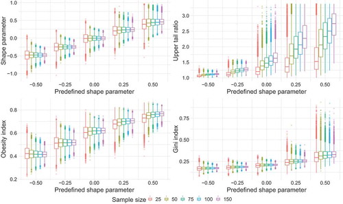
The bias, i.e. the difference in median estimates, introduced by the sample size, is relatively small for the shape parameter, obesity and Gini indices and hardly changes with increasing parent shape parameter. On the contrary, the median of UTR shows a high sensitivity to the sample size. The impact of the sample size on UTR strongly increases with increasing parent shape parameter. With increasing sample size the chance of encountering higher extraordinary events, i.e. record events, is increasing particularly for heavy-tailed distributions (Douglas and Vogel 2006, Smith et al. 2018). For the three indicators other than UTR, the sampling uncertainty decreases with increasing sample size. The UTR exhibits a strongly increasing sampling uncertainty for parent shape parameters ≥ 0.

The discriminative power is highest for the shape parameter and obesity index and is much lower for the Gini index and UTR. This can be observed from the distance between boxes for different parent shape parameters (Fig. 2). For instance, it is quite likely to obtain the same Gini index for observed samples with a wide range of tail heaviness of the parent distribution. The problem is aggravated for small sample sizes. For the shape parameter and obesity index, in contrast, the median for heavy-tailed distributions (e.g. ξ = 0.25) lies beyond the interquartile range for the Gumbel parent distribution (ξ = 0), even for small sample sizes.

The results show that all indicators reflect the tail heaviness defined by the shape parameter of the parent distribution to a different extent. With the exception of UTR, all indicators show a low sensitivity to the sample size. In practice this hampers the comparability of the UTR values across various locations with different record lengths. Moreover, the discriminative power for tail heaviness is found to be the smallest for UTR and Gini index (in this order), which may result in a wrong estimation of tail heaviness. The large sampling uncertainty associated with the UTR for heavy-tailed distributions additionally challenges the application of this indicator for the characterization of hydro-meteorological records.

3.1.2 Sensitivity to shifting the location parameter and to scale changes

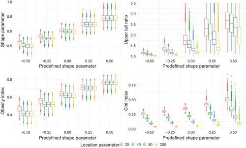
The mean of records (e.g. maximum annual precipitation or discharge) varies across different locations. When comparing different locations, it is a desirable property of an upper tail indicator to be invariant to shifts in the mean. Our bootstrap experiments show that changing the location parameter, while keeping the scale parameter constant, influences the four indicators differently (Fig. 3). While the shape parameter and the obesity index are nearly unaffected, the UTR and the Gini index respond strongly to shifts of the location parameter (and thus, to changes in the ratio of scale and location). For the latter two indicators, the median and the sampling uncertainty decrease with larger location parameters. The differences are particularly significant for the Gini index. Apparently, the σ/µ ratio affects the occurrence probability of large events, and the Gini and UTR are sensitive to the different resulting sampling distributions. The shape parameter and the obesity index are relatively unaffected by the σ/µ ratio. The analysis is additionally performed with constant location parameters and changing scale parameters (results not shown). The results are qualitatively similar but reverse as the Gini index and UTR increase with increasing scale parameters.

Figure 3. Boxplots of upper tail indicators for synthetic sampling distributions with sample size of 100, varying location parameter (20, 40, 80 and 200) and a constant scale parameter of 16.

The analysis shows that the shape parameter and obesity index are nearly invariant to changes in the ratio of location and scale parameters. They retain their discriminative power and show reasonable uncertainty for the predefined shape parameters. The situation is different for the Gini index and UTR, which questions the comparability when the Gini index and UTR are applied across different locations.

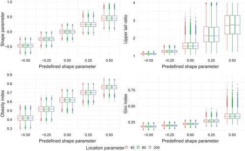
The four indicators are not sensitive to shifts in both parameters, as long as the σ/µ ratio is constant (Fig. 4). Smith et al. (2018) showed that the location and scale parameters of flood records are linearly related and the σ/µ ratio tends to be invariant across catchment scales. Under this assumption, all four upper tail indicators can be employed across scales. For comparability of the Gini index and UTR across locations, the invariance of σ/µ ratio needs to be taken into consideration.

Figure 4. Boxplots of upper tail indicators for synthetic sampling distributions with sample size of 100, varying location parameter (20, 40 and 200) and constant σ/µ ratio.

3.2 Analysis of the surprise factor as benchmark for heavy tail behaviour

In this section we use the previously defined surprise factor as a benchmark for tail heaviness. Two different distribution types – the two-parameter lognormal and the GEV distribution – are utilized as “true” distributions.

3.2.1 Lognormal distributions

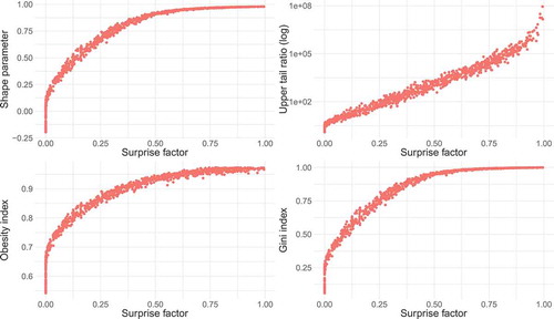
The relationship between the surprise factor and the four indicators computed for “true” distributions from the parent lognormal distributions is shown in Fig. 5. All four indicators show an increase for increasing surprise factors. However, the Gini index and the shape parameter show very little variation for very high surprise factors above 0.5, which correspond to extremely high shape parameters above 0.9. The UTR values increase monotonically but are highly dispersed (note the log scale of the y axis). For surprise factors around 0, the shape parameter, obesity index and Gini index show high variability and seem to discriminate the tail heaviness above a specific threshold (0.7, 0.2 and 0.25, respectively). Overall, these three indicators exhibit a similar relationship to the surprise factor.

Figure 5. Scatter plots of upper tail indicator vs surprise factor for 10³ synthetic “true” distributions drawn from parent lognormal distributions. Each of the 10⁴ sampling distributions from the “true” distribution contains 50 values and the surprise factor is estimated for a 50-year event with α = 1.5.

3.2.2 GEV distributions

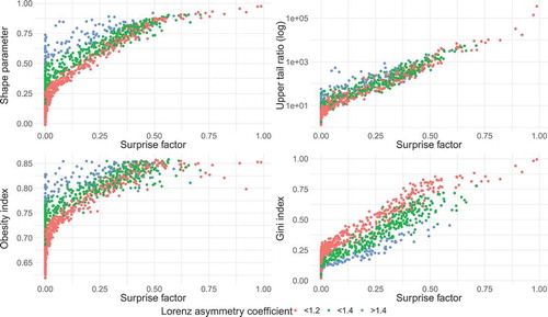
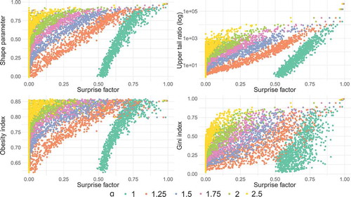
For the GEV parent distribution, all four indicators show an increasing tendency with increasing surprise factor, similarly to the case of lognormal distribution. However, a much greater dispersion is apparent for the GEV case. For instance, shape parameters for small surprise factors range from 0 to 0.75. When coloured according to their Lorenz asymmetry coefficients L, the values of all four indicators clearly differentiate (Fig. 6). The Lorenz asymmetry coefficient for the GEV-distributed samples has a wide range from 0.98 to 1.66, whereas L = 1 for the lognormal distribution. Hence, the Lorenz asymmetry coefficient explains the dispersion in the relation of the four indicators to the surprise factor. For nearly symmetric Lorenz curves (L < 1.2), the relationship between the Gini index, shape parameter, obesity index and the surprise factor are similar as was also observed in the lognormal case. The differences between the three indicators emerge with increasing Lorenz asymmetry coefficients. Here, the Gini index stands out as it behaves differently in relation to the Lorenz asymmetry coefficients. For example, samples with higher Lorenz asymmetry coefficient (blue dots) tend to have lower Gini indices. The shape parameter, obesity index and UTR tend to show the reverse behaviour. The highest surprise factors result from samples with the Lorenz asymmetry coefficients below 1.2.

Figure 6. Scatter plots of upper tail indicator vs surprise factor f or 10³ synthetic “true” distributions drawn from parent GEV distributions. Each of the 10⁴ sampling distributions from the “true” distribution contains 50 values and the surprise factor is estimated for a 50-year event with α = 1.5.

In order to better resolve the behaviour of upper tail indicators in relation to the surprise factor and Lorenz asymmetry coefficient, we depict them in the Lorenz space (Fig. 7; this figure corresponds to Fig. 1). Each point characterizes a “true” distribution drawn of the parent GEV distribution and corresponds to a specific Lorenz curve. We can position the point of the Lorenz curve with the maximum distance to the line of equality (y = x) in the Lorenz space. This point corresponds to the inflection point of the Lorenz curve. The distance between this point and the line of symmetry (y = −x + 1) indicates the Lorenz asymmetry coefficient. In Fig. 7, points are coloured according to the value of the upper tail indicators, the surprise factor and the Lorenz asymmetry coefficient.

Figure 7. Upper tail indicators, surprise factor and Lorenz asymmetry coefficient of the synthetic “true” distributions plotted in the Lorenz space. Each point represents the point of maximum distance to the line of equality (inflection point of the Lorenz curve) of one GEV distribution and is coloured according to the selected parameter in the respective legend. The division into classes of the Lorenz asymmetry coefficient is illustrated on the bottom right.

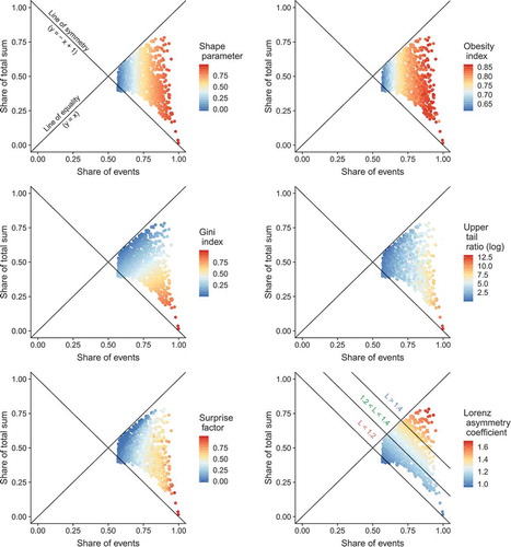
All four indicators show distinct gradients in different directions. While the shape parameter and the obesity index mainly depend on the position of the inflection point in the direction of the x axis, the Gini index increases orthogonally to the line of equality and the gradient of the log-scaled UTR points in a direction between these two. Comparing all four indicators, the pattern of the log UTR seems to follow closest the pattern of the surprise factor, though the high uncertainty of UTR is apparent through the mixed (non-smooth) colour pattern. For example, for UTR orange and blue points are mixed, the Gini pattern is on the contrary the smoothest one. It means that for samples with similar Lorenz curves, one can obtain quite different UTR, but similar Gini indices. The shape parameter and the obesity index also show rather smooth patterns in the Lorenz space.

All four upper tail indicators exhibit high values for points in the lower right corner of the Lorenz space, similar to the surprise factor. (Note that the colour of points should not be directly compared, but rather the relative change in the colours.) The Gini index mainly deviates from the surprise factor in the region of highly asymmetric Lorenz curves (L > 1.4), where small Gini indices are computed due to the small area between Lorenz curve and the line of equality. The distributions with L > 1.4 can however have high surprise factors (Fig. 7). Here, the shape parameter and the obesity index are more conservative and indicate high values, thus overestimating the surprise factor. Also, for the points close to the line of symmetry, the shape parameter and obesity index seem to overestimate the degree of surprise, i.e. tail heaviness, whereas the Gini index and UTR resemble the pattern of the surprise factor more closely.

Comparing the plots for shape parameter and obesity index (Fig. 7), it is apparent that samples with shape parameters between 0 and about 0.4 possess obesity indices below 0.75. This value is described to characterize the exponential distribution, which is a limiting case for heavy tail behaviour (Cooke et al. 2014). This reveals the weakness of the obesity index to identify GEV distributed samples with moderate shape parameters in the range between 0 and 0.4 as heavy-tailed.

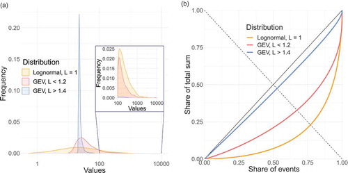
In order to illustrate the influence of different Lorenz asymmetry coefficients on the characteristics of the upper tail indicators, three example realizations are illustrated in Fig. 8 and corresponding parameters are given in Table 3. These samples are subjectively chosen and are characterized by similar shape parameters and obesity indices and similar magnitudes of location parameters but large differences in surprise factors. The blue and the red curves are samples from the GEV distributions with asymmetric and symmetric Lorenz curves, respectively, and the orange curve corresponds to the lognormal distribution (L = 1).

Table 3. Characteristics of the three example distributions of Fig. 8.

Parameter	Lognormal (orange)	GEV (red)	GEV (blue)
Shape parameter	0.63	0.61	0.62
Obesity index	0.85	0.79	0.81
Gini index	0.70	0.48	0.09
Upper tail ratio	43	168	20
Surprise factor (α = 1.5)	0.22	0.31	0.00
L	1.00	1.18	1.49
$X_{50\mathrm{y}\mathrm{r}}^{\mathrm{t}\mathrm{r}\mathrm{u}\mathrm{e}}$	367	235	39
σ	155.9^a	13	1
μ	57.8^a	26	22
σ/μ	2.70^a	0.50	0.05

^aFor the lognormal distribution, standard deviation, mean and coefficient of variation are given.

Although the location parameters of all three distributions are of similar magnitude, their variance is very different, which influences the probability of extremes in the upper tail. The different spread of extremes is also apparent in the corresponding Lorenz curves. The red and orange distributions have few extremes that account for ≥25% of the total sum. In contrast, the extremes in the tail of the blue distribution have little impact on the total sum and the Gini index is thus rather small (Fig. 8). The surprise factor is highest for the red curve and is 0 for the blue. The shape parameter and obesity index show high values and are similar for all three realizations. These two indicators mainly respond to the skewness of the distribution and have high values even if there are only few extremes in the tail. In this case they are not able to discriminate between the tail heaviness of the distributions. The UTR values show the same rank as those of the surprise factor (Table 3). In contrast, the Gini index shows a different ranking. It increases with a rising proportion of extremes in the total sum of event magnitudes. This effect can be caused by very few, very high extremes as well as by a few, less extreme but large events.

Figure 8. Three example distributions: density plots with log-scaled x axis (left) and the corresponding Lorenz curves (right).

3.2.3 Sensitivity of indicators to the degree of surprise α

The calculation of the surprise factor requires the choice of a degree of surprise α. For the surprise analysis we set α = 1.5, i.e. the probability of a $X_T^{\mathrm{t}\mathrm{r}\mathrm{u}\mathrm{e}}$ being 50% larger than estimated from observations. To examine the effect of α, each of the 10³ realizations is plotted according to the corresponding α values (Fig. 9). For different α values distinct patterns of upper tail indicators emerge; α controls the threshold at which the indicators start to monotonically increase with increasing surprise factor. With increasing degree of surprise beyond 1, the range of surprise factor values decreases, i.e. the probability of surprise gets smaller. The chosen value of α = 1.5 applied to the 50-year event appears reasonable from the engineering perspective and it seems to provide a good basis for comparison of the indicators through the well-resolved patterns. The introduced surprise factor is an intuitive measure of the consequences of heavy tails for engineering design and risk.

Figure 9. GEV-based surprise analysis with different degrees of surprise α.

4 Discussion

Our analyses indicate that the selected upper tail indicators are related to tail heaviness as they increase monotonically with increasing shape parameter of the parent GEV distribution and with increasing surprise factors for lognormal and GEV parent distributions. For distributions with nearly symmetric Lorenz curves (L < 1.2), all four indicators show a similar pattern to the surprise factor (Fig. 7). The main differences emerge for distributions with asymmetric Lorenz curves (L > 1.2). While the Gini index tends to underestimate the tail heaviness for asymmetric Lorenz curves (L > 1.2) compared to the ones with L < 1.2, the shape parameter and the obesity index exhibit an overestimation (Fig. 7). The UTR resembles best the pattern of the surprise factor in the Lorenz space. However, it possesses a number of unfavourable properties that impede its comparability across different locations, such as its strong sensitivity to the sample size.

In our synthetic experiments, we carried out analyses for stationary flood series. Non-stationarities may affect the upper tail indicators if, for instance, an underlying trend leads to events far above the previously observed. Upper tail indicators characterize the tail of frequency distributions that are constructed based on the assumption of independent, identically distributed values. If the assumption does not hold, the results should be interpreted in this context or time series need to be shortened to fulfil the assumption.

In the following, the main results are discussed for each upper tail indicator.

4.1 Shape parameter

The shape parameter is the only parametric upper tail indicator among the four investigated ones. Its application assumes that the sample belongs to a GEV distribution and this its main weakness. The shape parameter delivers a plausible description of tail heaviness also for samples drawn from the lognormal distribution. The shape parameter exhibits a number of favorable properties. It is found scale invariant and not sensitive to changes in the σ/µ ratio since it mainly responds to the skewness of the distribution and less to its dispersion. Furthermore, the shape parameter showed a relatively low sensitivity to the sample size, relatively high discrimination power and reasonable uncertainty compared to other indicators. It can thus be compared across sites with variable statistical moments and record lengths.

4.2 Obesity index

The obesity index shows a very similar behaviour as the shape parameter but has the advantage to be a non-parametric upper tail indicator. It was also found to be scale invariant and robust to changes in the σ/µ ratio and sample size. The sampling uncertainty of the obesity index is slightly larger than for the shape parameter, but overall the discriminative power is comparable. Cooke et al. (2014) proposed the threshold of 0.75 for heavy-tailed distributions. In their study, Cooke et al. (2014) justified this threshold with the definition of heavy-tailed distributions decreasing slower than exponential distributions. In our surprise analysis, we find obesity indices below the threshold of 0.75 for shape parameters between 0 and about 0.4 and surprise factors above 0. However, both shape parameter and obesity index show weaknesses by overestimating the tail heaviness expressed by the surprise factor for samples with asymmetric Lorenz curves (L > 1.2) (Figs. 7 and 8).

4.3 Gini index

The median of the Gini index has small sensitivity to the sample size, whereas the sampling uncertainty is larger for samples with positive shape parameters of the parent GEV distribution. It shows moderate discriminative power. The Gini index is found to be scale invariant, i.e. independent to changes in location with the σ/µ ratio being constant. It is however strongly sensitive to changes of the latter. Gini indices can thus be compared across sites and records if the σ/µ ratio can be assumed to be constant. For instance, Smith et al. (2018) found for annual peak flow records at >5500 gauges in the USA, that σ/µ is about 0.5 with a high degree of correlation between σ and µ. According to this finding, the applicability of the Gini index for the comparative analysis of tail heaviness is promising. Our analyses shows that the Gini index is less sensitive to tails with few (and relatively nearby) extremes (the blue distribution in Fig. 8). This is in agreement with studies by Cowell and Flachaire (2007) and McAleer et al. (2017). The Gini index detects heavy tails in case the extremes account for a considerable share of the total sum, caused by either one event or several events. The Gini index, however, underestimates the tail heaviness, i.e. surprise factors, for samples with asymmetric Lorenz curves (L > 1.2).

4.4 Upper tail ratio

The UTR is highly sensitive to the sample size which is in agreement with Smith et al. (2018). It directly depends on the flood of record, which varies with the record length (Douglas and Vogel 2006, Smith et al. 2018). The chance to observe extraordinary extremes increases with record length. The UTR shows the largest sampling uncertainty and the lowest discriminative power, i.e. the same value of UTR can be obtained for relatively light-tailed and heavy-tailed distributions depending on the record length. Though being scale invariant, it exhibits a high sensitivity to the location parameter. In overall, the comparability of UTR across different locations and records is limited. At the same time, the logarithm of the UTR seems to have the closest pattern to the surprise factor (Fig. 7). Hence, it can be applied when comparing records of similar length and with nearly constant σ/µ ratio, however, the high sampling uncertainty should be kept in mind.

5 Conclusions and recommendations

This paper presents the first comparative analysis of four scalar upper tail indicators: the shape parameter of the generalized extreme value distribution, the obesity index, the Gini index and the upper tail ratio. We analysed their sensitivity to the sample size, to changes in the location parameter with variable σ/µ ratio and to changes in scale with constant σ/µ ratio. This analysis elucidates the comparability of the indicators across various sites and record lengths. Further, we propose a surprise factor as a synthetic benchmark for upper tail heaviness. It is related to implications of tail heaviness for hydrological engineering design and risk. The benchmark analysis reveals different patterns of the upper tail indicators in relation to the pattern of the surprise factor in the Lorenz space. We conclude the following:

1. The median estimates for all indicators except UTR show little sensitivity to the sample size.

2. The sampling uncertainty for heavy-tailed distributions is highest for UTR, followed by Gini index, obesity index and shape parameter.

3. All indicators are scale invariant, i.e. they are insensitive to changes in location and scale parameters subject to a constant σ/µ ratio.

4. Shape parameter and obesity index exhibit little sensitivity to changes in location with variable σ/µ ratio, whereas Gini index and UTR are highly sensitive.

5. The logarithmic UTR seems to resemble the pattern of the surprise factor best.

6. The patterns of the shape parameter, obesity index and Gini index are similar for samples characterized by nearly symmetric Lorenz curves with Lorenz asymmetry coefficient (L < 1.2).

7. Obesity index appears to classify GEV distributed samples with the shape parameters between 0 and about 0.4 as light-tailed (obesity index < 0.75).

8. For samples with asymmetric Lorenz curves (L > 1.2), the Gini index seems to underestimate the tail heaviness, i.e. the surprise factor, whereas the shape parameter and the obesity index tend to overestimate the surprise factor compared to samples with lower Lorenz asymmetry coefficients.

Our results show that there is no perfect upper tail indicator. All indicators have specific advantages and disadvantages. For analysis of tail heaviness, where the surprise factor is taken as the benchmark, the UTR can be used for comparing records of similar lengths, but high sampling uncertainty should be kept in mind. Moreover, a constant σ/µ ratio needs to be assured for comparability of UTR across different locations. If sample size is different, which is often the case in practical applications, the combination of the GEV shape parameter, non-parametric obesity and Gini indices is recommended. Also, for the Gini index, similar σ/µ ratios are required for comparability across various locations. We further recommend that these indices are accompanied by the Lorenz asymmetry coefficients. For samples characterized by asymmetric Lorenz curves, the Gini index shows a divergent tendency compared to other two. The results for such samples need to be interpreted with care, taking into account the over- and underestimation tendencies of the indices, compared to the samples with symmetric Lorenz curves.

Disclosure statement

No potential conflict of interest was reported by the authors.

Additional information

Funding

The financial support of the German Research Foundation (Deutsche Forschungsgemeinschaft, DFG) in terms of the research group FOR 2416 “Space-Time Dynamics of Extreme Floods (SPATE)” is gratefully acknowledged.

References

- Barth, N.A., Villarini, G., and White, K., 2019. Accounting for mixed populations in flood frequency analysis: bulletin 17C perspective. Journal of Hydrologic Engineering, 24 (3), 1–12. doi:10.1061/(ASCE)HE.1943-5584.0001762
- Benhabib, J., Bisin, A., and Zhu, S., 2011. The distribution of wealth and fiscal policy in economies with finitely lived agents. Econometrica, 79 (1), 123–157.
- Bernardara, P., et al., 2008. The flood probability distribution tail: how heavy is it? Stochastic Environmental Research and Risk Assessment, 22 (1), 107–122. doi:10.1007/s00477-006-0101-2
- Bryson, M.C., 1974. Heavy-tailed distributions: properties and tests. Technometrics, 16 (1), 37–41. doi:10.1080/00401706.1974.10489150
- Canchola, J.A., 2018. Correct use of percent coefficient of variation (%CV) formula for log-transformed data. MOJ Proteomics & Bioinformatics, 6 (3), 316–317.
- Coles, S., 2001. An introduction to statistical modeling of extreme values. London: Springer Science & Business Media.
- Cooke, R.M. and Nieboer, D., 2011. Heavy-tailed distributions: data, diagnostics, and new developments. SSRN Electronic Journal, (March). doi:10.2139/ssrn.1811043
- Cooke, R.M., Nieboer, D., and Misiewicz, J., 2014. Fat-tailed distributions: data, diagnostics and dependence. Vol. 1. Hoboken, NJ: John Wiley & Sons.
- Cowell, F.A. and Flachaire, E., 2007. Income distribution and inequality measurement: the problem of extreme values. Journal of Econometrics, 141 (2), 1044–1072. doi:10.1016/j.jeconom.2007.01.001
- Crovella, M.E. and Taqqu, M.S., 1999. Estimating the heavy tail index from scaling properties. Methodology and Computing in Applied Probability, 1 (1), 55–79. doi:10.1023/A:1010012224103
- Damgaard, C. and Weiner, J., 2000. Describing inequality in plant size or fecundity. Ecology, 81 (4), 1139–1142. doi:10.1890/0012-9658(2000)081[1139:DIIPSO]2.0.CO;2
- Daníelsson, J., et al., 2001. Using a bootstrap method to choose the sample fraction in tail index estimation. Journal of Multivariate Analysis, 76 (2), 226–248. doi:10.1006/jmva.2000.1903
- Daníelsson, J., et al., 2006. Comparing downside risk measures for heavy tailed distributions. Economics Letters, 92 (2), 202–208. doi:10.1016/j.econlet.2006.02.004
- Douglas, E.M. and Vogel, R.M., 2006. Probabilistic behavior of floods of record in the United States. Journal of Hydrologic Engineering, 11 (5), 482–488. doi:10.1061/(ASCE)1084-0699(2006)11:5(482)
- El Adlouni, S., Bobée, B., and Ouarda, T., 2008. On the tails of extreme event distributions in hydrology. Journal of Hydrology, 355 (1–4), 16–33. doi:10.1016/j.jhydrol.2008.02.011
- Eliazar, I.I. and Sokolov, I.M., 2010. Gini characterization of extreme-value statistics. Physica A: Statistical Mechanics and Its Applications, 389 (21), 4462–4472. doi:10.1016/j.physa.2010.07.005
- Embrechts, P., Klüppelberg, C., and Mikosch, T., 2003. Modelling extremal events: for insurance and finance. Germany: Springer Berlin Heidelberg.
- Fisher, R.A. and Tippett, L.H.C., 1928. Limiting forms of the frequency distribution of the largest or smallest member of a sample. Mathematical Proceedings of the Cambridge Philosophical Society, 24 (2), 180–190. doi:10.1017/S0305004100015681
- Fontanari, A., Cirillo, P., and Oosterlee, C.W., 2018a. From concentration profiles to concentration maps. New tools for the study of loss distributions. Insurance: Mathematics and Economics, 78, 13–29.
- Fontanari, A., Taleb, N.N., and Cirillo, P., 2018b. Gini estimation under infinite variance. Physica A: Statistical Mechanics and Its Applications, 502, 256–269. doi:10.1016/j.physa.2018.02.102
- Foss, S., Korshunov, D., and Zachary, S., 2013. An introduction to heavy-tailed and subexponential distributions. New York, NY: Springer.
- Gnedenko, B., 1943. Sur la distribution limité du terme maximum d’une série aléatoire. Annals of Mathematics, 44 (3), 423–453. doi:10.2307/1968974
- Gu, X., et al., 2017. Spatiotemporal patterns of annual and seasonal precipitation extreme distributions across China and potential impact of tropical cyclones. International Journal of Climatology, 37 (10), 3949–3962. doi:10.1002/joc.4969
- Hosking, J.R.M., 1990. L-moments: analysis and estimation of distributions using linear combinations of order statistics. Journal of the Royal Statistical Society, Series B, 52 (1), 105–124.
- Jawitz, J.W. and Mitchell, J., 2011. Temporal inequality in catchment discharge and solute export. Water Resources Research, 47 (10), 1–16. doi:10.1029/2010WR010197
- Katz, R.W., 2002. Do weather or climate variables and their impacts have heavy-tailed distributions? In: 16th Conf. on Probability and Statistics in the Atmospheric Sciences, Orlando, FL. American Meteorological Society, J3.5.
- Katz, R.W., et al., 2005. Statistics of extremes: modeling ecological disturbances. Ecology, 86 (5), 1124–1134. doi:10.1890/04-0606
- Katz, R.W., Parlange, M.B., and Naveau, P., 2002. Statistics of extremes in hydrology. Advances in Water Resources, 25 (8–12), 1287–1304. doi:10.1016/S0309-1708(02)00056-8
- Konapala, G., Mishra, A., and Leung, L.R., 2017. Changes in temporal variability of precipitation over land due to anthropogenic forcings. Environmental Research Letters, 12 (2), 024009. doi:10.1088/1748-9326/aa568a
- Kondor, D., et al., 2014. Do the rich get richer? An empirical analysis of the Bitcoin transaction network. PLoS ONE, 9 (2), e86197. doi:10.1371/journal.pone.0086197
- Kousky, C. and Cooke, R.M., 2009. The unholy trinity: fat tails, tail dependence, and micro-correlations. Resources for the Future Discussion Paper, Washington, DC: Resources for the Future, 09-36.
- Kyselý, J., 2010. Coverage probability of bootstrap confidence intervals in heavy-tailed frequency models, with application to precipitation data. Theoretical and Applied Climatology, 101 (3–4), 345–361. doi:10.1007/s00704-009-0190-1
- Kyselý, J. and Picek, J., 2007. Regional growth curves and improved design value estimates of extreme precipitation events in the Czech Republic. Climate, 33 (3), 243–255.
- Lai, W., Wang, H., and Zhang, J., 2018. Comprehensive assessment of drought from 1960 to 2013 in China based on different perspectives. Theoretical and Applied Climatology, 134 (1–2), 585–594. doi:10.1007/s00704-017-2294-3
- Lu, P., et al., 2017. Spatial characterization of flood magnitudes over the drainage network of the Delaware River Basin. Journal of Hydrometeorology, 8 (4), 957–976. doi:10.1175/JHM-D-16-0071.1
- Makkonen, L., 2006. Plotting positions in extreme value analysis. Journal of Applied Meteorology and Climatology, 45 (2), 334–340. doi:10.1175/JAM2349.1
- Malamud, B., 2004. Tails of natural hazards. Physics World, 17 (8), 31–35. doi:10.1088/2058-7058/17/8/35
- Masaki, Y., et al., 2014. Global-scale analysis on future changes in flow regimes using Gini and Lorenz asymmetry coefficients. Water Resources Research, 50 (5), 4054–4078. doi:10.1002/2013WR014266
- McAleer, M., Ryu, H.K., and Slottje, D.J., 2017. A new inequality measure that is sensitive to extreme values and asymmetries. Tinbergen Institute Discussion Paper, 1725, 2341–2356.
- Merz, B., et al., 2015. Charting unknown waters - on the role of surprise in flood risk assessment and management. Water Resources Research, 51 (8), 6399–6416. doi:10.1002/2015WR017464
- Mikosch, T., 1999. Regular variation, subexponentiality and their applications in probability theory. Report Eurandom, 99013, 13.
- Morrison, J.E. and Smith, J.A., 2002. Stochastic modeling of flood peaks using the generalized extreme value distribution. Water Resources Research, 38 (12), 1–12. doi:10.1029/2001WR000502
- Naghettini, M., Potter, K.W., and Illangasekare, T., 1996. Estimating the upper tail of flood-peak frequency distributions using hydrometeorological information. Water Resources Research, 32 (6), 1729–1740. doi:10.1029/96WR00200
- Nerantzaki, S. and Papalexiou, S.M., 2019. Tails of extremes: advancing a graphical method and harnessing big data to assess precipitation extremes. Advances in Water Resources, 134, 103448. doi:10.1016/j.advwatres.2019.103448
- Nordhaus, W.D., 2011. The economics of tail events with an application to climate change. Review of Environmental Economics and Policy, 5 (2), 240–257. Oxford University Press. doi:10.1093/reep/rer004
- Papalexiou, S.M., AghaKouchak, A., and Foufoula-Georgiou, E., 2018. A diagnostic framework for understanding climatology of tails of hourly precipitation extremes in the United States. Water Resources Research, 54 (9), 6725–6738. doi:10.1029/2018WR022732
- Papalexiou, S.M. and Koutsoyiannis, D., 2013. Battle of extreme value distributions: A global survey on extreme daily rainfall. Water Resources Research, 49 (1), 187–201. doi:10.1029/2012WR012557
- Papalexiou, S.M., Koutsoyiannis, D., and Makropoulos, C., 2013. How extreme is extreme? An assessment of daily rainfall distribution tails. Hydrology and Earth System Sciences, 17 (2), 851–862. doi:10.5194/hess-17-851-2013
- Rajah, K., et al., 2014. Changes to the temporal distribution of daily precipitation. Geophysical Research Letters, 41 (24), 8887–8894. doi:10.1002/2014GL062156
- Reiss, R.D. and Thomas, M., 2007. Statistical analysis of extreme values: with applications to insurance, finance, hydrology and other fields. 3rd ed. Basel: Birkhäuser.
- Resnick, S.I., 2007. Heavy-tail phenomena: probabilistic and statistical modeling. New York, NY: Springer Science & Business Media.
- Sartori, M. and Schiavo, S., 2015. Connected we stand: A network perspective on trade and global food security. Food Policy, 57, 114–127. doi:10.1016/j.foodpol.2015.10.004
- Smith, J.A., et al., 2018. Strange floods: the upper tail of flood peaks in the United States. Water Resources Research, 54 (9), 6510–6542. doi:10.1029/2018WR022539
- Smith, J.A., Villarini, G., and Baeck, M.L., 2011. Mixture distributions and the hydroclimatology of extreme rainfall and flooding in the Eastern United States. Journal of Hydrometeorology, 12 (2), 294–309. doi:10.1175/2010JHM1242.1
- Taleb, N.N., 2007. The Black Swan: the impact of the highly improbable. New York, NY: Random House.
- Villarini, G. and Smith, J.A., 2010. Flood peak distributions for the eastern United States. Water Resources Research, 46 (6), 1–17. doi:10.1029/2009WR008395
- Villarini, G., et al., 2011a. Characterization of rainfall distribution and flooding associated with U.S. landfalling tropical cyclones: analyses of Hurricanes Frances, Ivan, and Jeanne (2004). Journal of Geophysical Research: Atmospheres, 116 (D23), D23. doi:10.1029/2011JD016175
- Villarini, G., et al., 2011b. On the frequency of heavy rainfall for the Midwest of the United States. Journal of Hydrology, 400, 103–120.
- Werner, T. and Upper, C., 2002. Time variation in the tail behaviour of bund futures returns. Discussion Paper, Economic Research Centre of the Deutsche Bundesbank, 25 (2), 1–36.
- Zhang, Q., et al., 2015. Homogenization of precipitation and flow regimes across China: changing properties, causes and implications. Journal of Hydrology, 530, 462–475. doi:10.1016/j.jhydrol.2015.09.041
- Zhou, Z., et al., 2017. The complexities of urban flood response: flood frequency analyses for the Charlotte metropolitan region. Water Resources Research, 53 (8), 7401–7425. doi:10.1002/2016WR019997