Inter- and intra-annual trend analysis of water level and flow in the middle and lower reaches of the Ganjiang River, China

ABSTRACT

The Ganjiang River is the largest tributary of Poyang Lake in China, and its hydrological regime variation greatly affects the utilization of regional water resources and the ecological environment of the lake. In this study, a novel trend analysis method, the Moving Average over Shifting Horizon (MASH), was applied to investigate the inter- and intra-annual trends of flow and water level from 1976 to 2016 at the Xiajiang and the Waizhou hydrological stations in the Ganjiang River. The Significant Change Rate Method (SCRM) was proposed to determine the MASH averaging parameters. The trend analysis results show a statistically significant decrease in water level series throughout the year and the relationship of flow and water level have changed greatly at the Waizhou station. The sediment load reduction, large-scale sand mining and water level decrease of Poyang Lake are identified as the main causes for the water level decrease.

KEYWORDS:

• trend analysis
• Moving Average over Shifting Horizon (MASH)
• Significant Change Rate Method (SCRM)
• Mann-Kendall trend test
• water level
• flow
• Ganjiang River, China

Editor A. Fiori Associate editor K. Ryberg

1 Introduction

Poyang Lake lies in the middle reach of the Yangtze River, China. It is the largest freshwater lake in China, with a catchment area of 162 000 km² (Shankman et al. 2010). The major functions of the lake include ecological security, hydrological adjustment and climate regulation. These functions are important for the Jiangxi Province and other regions in the middle and lower reaches of the Yangtze River (Zhang et al. 2014, Yang et al. 2019). Poyang Lake has five tributaries; the inflows from them into the lake primarily drive the seasonal variations in the water level of the lake and the water resource (Hu et al. 2007, Li and Zhang 2018).

The Ganjiang River is one of the eight major tributaries of the Yangtze River (Wang et al. 2017) and the Ganjiang River Basin is also the largest sub-basin of the Poyang Lake (Zhang et al. 2017b). The hydrological regime changes of Poyang Lake relate to the hydrological variations in the Ganjiang River. Climate change and human activities, such as land-use and land cover change, have influenced variations in flow over the past few decades (Tu et al. 2015, Zhang et al. 2016, 2019). Climate change may influence regional hydrological cycles by altering precipitation, temperature and evapotranspiration, thus causing alteration in the river flow (Walling 1983, Guo et al. 2019). Some researchers (Allan and Soden 2008, Li et al. 2015) have found that climate warming has led to more frequent extreme precipitation events. In addition, while human activities, such as hydro-project construction, provide economic and social benefits (Yu et al. 2014, Alrajoula et al. 2016), these activities also alter the natural hydrological regime in the magnitude, timing, duration, frequency and rate of water condition changes (Cardwell et al. 1996, Richter et al. 1996, Poff et al. 1997, Benjamin and Vankrik 1999, Yang et al. 2008).

Previous research on the influence of climate change on the Ganjiang River revealed that annual flow has not statistically significantly changed in this region (Huang et al. 2019, Guo et al. 2019) in recent decades, while there is more frequent occurrence of flooding and drought disasters in the Poyang Lake catchment (Zhang et al. 2015, 2017a). As for human activities, many hydro-projects (e.g. dams or reservoirs) have been constructed along the Ganjiang River since the 1980s (Liu et al. 2016), possibly reducing high flows, increasing low flows (Yang et al. 2008, Magilligan et al. 2016, Huang et al. 2019) and reducing the sediment load downstream of dams (Wang et al. 2005, Fu et al. 2008, Song et al. 2018). In addition, increased sand mining over the past few decades has also led to a reduction in the sediment load in the lower reaches of the Ganjiang River (Chen et al. 2016, Wen et al. 2019). Low sediment load may strengthen the riverbed cutting-down processes, thus making the water level decrease. If the water level is lower than the design water-intake altitude, it is difficult for hydro-plants to get water from the river. In addition, if the water level in the middle and lower reaches of the Ganjiang River keeps falling, the waterway level becomes too low to be navigable by ship. Therefore, understanding and quantifying these variations and trends in the water level and flow is important for effective water resources management.

Many trend analysis techniques (Sonali and Kumar 2013) are used to study the time series of climatic variables (Oguntunde et al. 2011) and river streamflow (Rougé et al. 2013); these techniques include the Mann-Kendall (M-K) trend test, Spearman’s test and the moving t test. However, when time series have intra- and inter-annual variations, it is difficult for these traditional techniques to detect the intra- and inter-annual trends simultaneously. Given this, Anghileri et al. (2014) proposed a novel trend technique, called the Moving Average over Shifting Horizon (MASH). Osuch and Wawrzyniak (2016, 2017) then applied MASH to detect meteorological variables and snow-depth trends. MASH is shown to perform well in trend analysis of intra- and inter-annual time series; however, there is no general rule for selecting MASH averaging parameters, which requires further research (Anghileri et al. 2014). Therefore, in this study, we define an index θ, referred to as the significant change rate and propose an approach, the Significant Change Rate Method (SCRM), to help select the averaging parameters for MASH.

This study investigates the intra- and inter-annual trend of the water level and flow series in the middle and lower reaches of the Ganjiang River, applying the MASH method, the pre-whitening M-K trend test and Sen’s slope method, with SCRM to select the appropriate averaging parameters. MASH is applied to visually analyse the inter- and intra-trends in the water level and flow using the averaging parameters based on the results of SCRM. The M-K trend test and Sen’s slope method are also used to quantify the time series trends filtered by MASH. Then, the study compares the original flow and water level series trends with the trends of corresponding series smoothed by MASH. Finally, the study focuses on discussing the causes of water-level variability trends in the lower reaches of the Ganjiang River.

The rest of this paper is organized as follows: Section 2 introduces the study area and data; Section 3 describes the applied methods, including the pre-whitening M-K trend test, Sen’s method, SCRM and MASH for the time series trend analysis; Section 4 provides the results and discussion of trend analysis for water level and flow series at two hydrological stations; and Section 5 includes the conclusions of this study.

2 Study area and data

2.1 Study area

The Ganjiang River is located in the southern part of the middle reaches of the Yangtze River, with a length of 766 km and basin area of 83 500 km². The mean annual discharge of the Ganjiang River is 2130 m³/s. The basin is situated in the subtropical humid monsoon climate zone, with annual precipitation of approx. 1400–1800 mm. The mean annual temperature is 17.8ºC. Up to 2014, 4380 reservoirs were built in the basin, of which139 were large and medium reservoirs (Du et al. 2016). The largest reservoir is Wan’an Reservoir, with capacity storage of 22.8 × 10⁸ m³, and it started operation in 1990.

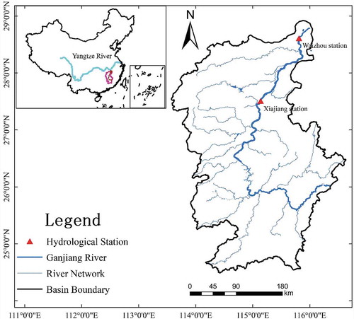
The data of two hydrological stations are studied: the Xiajiang hydrological station (Xiajiang County, Jiangxi Province, China), located in the middle to lower reaches of the Ganjiang River, which controls about 75% of the Ganjiang River basin area; and the Waizhou hydrological station (Nanchang City, Jiangxi Province, China), which is located at the outlet of the Ganjiang River. Waizhou station controls 97% of the Ganjiang River basin and its boundaries are at 113°42'E–116°38'E; 24°30'N–28°42'N (Zhang et al. 2017b). Figure 1 shows the location of the Ganjiang River basin and the two hydrological stations.

Figure 1. Location of the Ganjiang River basin in China and the Xiajiang and Waizhou hydrological stations.

2.2 Data

The data for this study were collected at the Xiajiang and Waizhou hydrological stations and included daily time series of water level and flow data. The time series data were from the start of 1976 to the end of 2016, a period of 41 years. The daily time series data of the water level and flow were obtained from the Jiangxi Provincial Institute of Water Sciences.

3 Methodology

3.1 Pre-whitening M-K trend test and Sen’s slope estimator

The Mann-Kendall (M-K) trend test (Mann 1945, Kendall 1975) is a popular rank-based nonparametric method for testing trends in time series for meteorological data (Li et al. 2017, Song et al. 2018). The M-K test applies to an independent time series. However, for a dependent series, a positive serial autocorrelation may increase the possibility that the M-K test detects trends in a non-trend series (Von Storch 1995). Therefore, before using the M-K trend test, this study considered pre-whitening the original time series to remove serial autocorrelation (Yue and Wang 2002), as follows:

(1) ${x_t}^{\mathrm{\prime }}=x_t-r_1{x}_{t-1}$(1)

where x_t represents the tth time interval of the original time series; x_t' represents the tth time interval of the pre-whitened series; and r₁ is the lag-1 autocorrelation coefficient of the sample data.

After removing serial autocorrelation from the original time series, the M-K trend test statistics S is calculated as:

(2) $S={\sum }_{j=k+1}^n{\sum }_{k=1}^{n-1}\mathrm{s}\mathrm{g}\mathrm{n}\left(x_j-x_i\right)$(2)

where x_i and x_j are the value of the pre-whitened time series in year i and j, respectively, with j > k; n is the total number of sample variables; and sgn(*) is calculated as:

(3) $\mathrm{s}\mathrm{g}\mathrm{n}(x_j>x_i)=\left\{\begin{array}{c}1\mathrm{f}\mathrm{o}\mathrm{r}{x}_j>x_i\\ 0\mathrm{f}\mathrm{o}\mathrm{r}{x}_j=x_i\\ -1\mathrm{f}\mathrm{o}\mathrm{r}{x}_j<x_i\end{array}\right.$(3)

The statistic S follows an approximately normal distribution, with mean E(S) = 0 and a variance var(S) = n(n−1)(2n + 5)/18. The standardized test statistic Z is calculated by:

(4) $Z=\left\{\begin{array}{c}\frac{S-1}{\sqrt{\mathrm{v}\mathrm{a}\mathrm{r}\left(S\right)}}\mathrm{f}\mathrm{o}\mathrm{r}S>0\\ 0\mathrm{f}\mathrm{o}\mathrm{r}S=0\\ \frac{S+1}{\sqrt{\mathrm{v}\mathrm{a}\mathrm{r}\left(S\right)}}\mathrm{f}\mathrm{o}\mathrm{r}S<0\end{array}\right.$(4)

A Z value greater or less than 0 indicates that there is an increasing or decreasing trend, respectively, in the time series. The significance in the trends can be identified by comparing the Z value with the standard normal variable U_1-α/2 at a given confidence level α. Normally, α is set at 0.05, which means U_1-α/2 = 1.96 at a 0.05 confidence level. If Z > 1.96 or < −1.96, there is a positive or negative significant trend, respectively, in the series. Otherwise, the trend is not statistically significant.

The magnitude of the trend of the series can be assessed using the non-parametric Sen slope estimator proposed by Sen (1968). This estimator is widely used to analyse trends in hydro-meteorological series (e.g. Gocic and Trajkovic 2013, Wang et al. 2019). The estimator assumes a linear trend; the trend slope is calculated by:

(5) $\beta =\mathrm{m}\mathrm{e}\mathrm{d}\mathrm{i}\mathrm{a}\mathrm{n}\left(\frac{x_j-x_i}{j-i}\right),\mathrm{\forall }j>i\left(i=1,2,\dots n-1;j=2,3,\dots n\right)$(5)

where x_j and x_i are data values at times j and i, respectively; and n is the length of the series. The median of the ascending sequence of values {(x_j−x_i)/(j−i)} reflects the Sen slope estimator. The confidence interval of the slope is calculated by:

(6) $\left\{\begin{array}{c}{C}_{\alpha }=U_{1-0.5\alpha }\sqrt{\mathrm{v}\mathrm{a}\mathrm{r}\left(S\right)}\\ M_1=\left(N-C_{\alpha }\right)/2\\ M_2=\left(N+C_{\alpha }\right)/2\\ P\left\{X_{\left(M_1\right)}<\beta <X_{\left(M_2+1\right)}|\beta \right\}=1-\alpha \end{array}\right.$(6)

where U_1-α is the standard normal variable at a given confidence level α and var(S) = n(n−1)(2n + 5)/18. The variable N = (n−1)n/2 is the length of the series [(x_j−x_i)/(j−i)], written as X: X_(M1) and X_(M2+1). These are the M₁th and (M₂ + 1)th values in the ascending sequence X, respectively, and the terms represent the lower and upper limits of coincidence intervals for the slope estimator β. The variable α is the confidence level and usually, the value is 0.05.

3.2 Moving Average over Shifting Horizon (MASH)

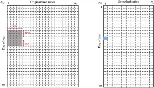
The Moving Average over Shifting Horizon (MASH) method is a novel approach to exploratory data analysis (EDA), proposed by Anghileri et al. (2014). MASH can simultaneously address the seasonality and inter-annual variability of time series. Figure 2 illustrates the MASH procedure, in which the original time series (the rectangle on the left) are transformed into the smoothed series (the rectangle on the right). This approach is a moving-average method that considers two dimensions: over the same days in consecutive years and over consecutive days in the same year. MASH is constructed as a matrix, as follows:

(7) $\left[\begin{array}{c}\begin{array}{cc}{u}_{1,1}& u_{1,2}\\ u_{2,1}& u_{2,2}\end{array}\\ \begin{array}{cc}\dots & \dots \\ u_{365,1}& u_{365,2}\end{array}\end{array}\begin{array}{c}\begin{array}{cc}\dots & u_{1,N_h}\\ \dots & u_{2,N_h}\end{array}\\ \begin{array}{cc}\dots & \dots \\ \dots & u_{365,N_h}\end{array}\end{array}\right]$(7)

Figure 2. Schematic representation of averaging applied in the MASH method for parameters, Y = 5 and w = 2. The term μ_t,_h represents the average daily data on the tth day in the year of hth horizon and x_d,_y represents the data on the dth day of the yth year of the time series. In this example, the data are averaged over 5 days (2w + 1) and 5 years (Y) is shown as a shaded rectangle.

In this matrix, the columns are the mean of the time series seasonal patterns, calculated over different horizons, N_h. The term μ_t,_h represents the average daily data on the tth day in the year of hth horizon, calculated as:

(8) $u_{t,h}=\mathrm{m}\mathrm{e}\mathrm{a}{\mathrm{n}}_{y\in \left[h,h+Y-1\right]}\left[\mathrm{m}\mathrm{e}\mathrm{a}{\mathrm{n}}_{d\in \left[t-w,t+w\right]}\left(x_{d,y}\right)\right]$(8)

where x_d,_y represents the data on the dth day of the yth year of the time series; and w and Y are two averaging parameters of MASH, which influence the averaging result. The number of N_h horizons is related to Y, which is computed as N_h = N_y−Y + 1, where N_Y represents the length of the original time series.

In Equation (8)(8) $u_{t,h}=\mathrm{m}\mathrm{e}\mathrm{a}{\mathrm{n}}_{y\in \left[h,h+Y-1\right]}\left[\mathrm{m}\mathrm{e}\mathrm{a}{\mathrm{n}}_{d\in \left[t-w,t+w\right]}\left(x_{d,y}\right)\right]$(8) , the averaging parameter w reflects the result of the intra-annual smoothing, and Y shows the effect of the inter-annual smoothing. If the parameter w is too small, the day-to-day variability may not be smoothed out and the seasonal pattern may not emerge. If w is too large, the seasonal variation may be over-smoothed (Osuch and Wawrzyniak 2016). If the parameter Y is too large, the length of smoothed series may be too short, and the statistical significance may be weakened (Anghileri et al. 2014). If Y is too small, the inter-annual characteristics of the time series may not appear.

Given the limitations associated with determining the appropriate MASH averaging parameters, this study uses the SCRM to help select w and Y.

3.3 Significant change rate method

Anghileri et al. (2014) and Osuch and Wawrzyniak (2016) recommended using a sensitivity analysis, fixing one parameter and changing the other, combined with a statistical method, to assess the influence of different Y and w values on the MASH analysis. However, both parameters cannot be changed at the same time using this method. If the Y and w sample sizes are not big enough, the appropriate averaging parameters may be missed. This study takes different values of Y and w and uses Eq. (8)(8) $u_{t,h}=\mathrm{m}\mathrm{e}\mathrm{a}{\mathrm{n}}_{y\in \left[h,h+Y-1\right]}\left[\mathrm{m}\mathrm{e}\mathrm{a}{\mathrm{n}}_{d\in \left[t-w,t+w\right]}\left(x_{d,y}\right)\right]$(8) to obtain MASH matrices. An index defined as significant change rate θ is established to evaluate the impact of different Y and w values on the MASH analysis. According to the relationship of θ, Y and w, the averaging parameters may be determined for MASH. The calculation procedures are as follows:

Step 1. Calculate the MASH matrixes based on different w and Y values.

Assume the MASH averaging parameter w = 1, 2, …, N, Y = 1, 2 … M. Then, apply the MASH method to process the original time series to get MASH matrices, the number of which is M × N.

Step 2. Use the pre-whitening M-K trend test to compute significant change days.

Apply the pre-whitening M-K trend test for each row of data in each MASH matrix to calculate the days with significant changes. The days with significant changes are identified by:

(9) $D_{i,j}={\sum }_{k=1}^{365}\mathrm{s}\mathrm{g}\mathrm{n}(\left|Z_{i,j,k}\right|-U_{1-0.5\alpha })$(9)

where D_i,_j represents the days with significant changes, with Y = i and w = j. The static Z_i,_j,k (i = 1, 2, …, M; j = 1, 2, …, N; k = 1, 2, …, 365), represents the pre-whitening M-K trend test result of the kth row of the MASH matrix, with Y = i and w = j. The term U_1−0.5α is the value of standard normal variate at a given confidence level α. The sgn(*) function is calculated as:

(10) $\mathrm{s}\mathrm{g}\mathrm{n}\left(x\right)=\left\{\begin{array}{c}1\mathrm{f}\mathrm{o}\mathrm{r}x\ge 0\\ 0\mathrm{f}\mathrm{o}\mathrm{r}x<0\end{array}\right.$(10)

Step 3. Compute the significant change rate to help select the averaging parameters Y and w.

Define the significant change rate θ_i,_jas:

(11) ${\theta }_{i,j}=\frac{D_{i,j}}{365}\left(i=1,2,\dots M,j=1,2,\dots ,N\right)$(11)

where θ_i,_j indicates the ratio of the number of the days with significant changes to the total number of days of a year, with Y = i and w = j.

Step 4. Plot θ with Y and w to help select the averaging parameter.

This study assumes a relationship between θ and the averaging parameters. In other words, when the value of Y and w is determined, the value of θ is also certain. A larger θ value indicates that the trend represented by the MASH smoothed time series is clearer. Then, the selected corresponding Y and w values for the larger θ are considered as the averaging parameters. The relationship between θ and the averaging parameters is determined by establishing Y and w as the transverse and vertical axes, respectively, to plot θ with Y and w. Next, the corresponding Y and w of the largest θ are selected as the averaging parameters. If there is more than one maximum value of θ, this means that the impact of different Y and w pairs is equifinal for the MASH analysis; therefore, any pair of Y and w from the maximum values of θ can be selected as averaging parameters. The structure diagram of this study is shown in Fig. 3.

Figure 3. Structure diagram of the study.

4 Results and discussion

4.1 Results of MASH averaging parameter selection

The SCRM was used to select a pair of appropriate MASH averaging parameters, Y and w. Based on the length of the researched time series (1976–2016), we set Y = 1, 2,…, 30 and w = 1, 2,…, 30. This allowed us to compute 900 significant change rate values of θ using SCRM. Figure 4 shows the SCRM results for water level and flow at both Xiajiang and Waizhou hydrological stations.

Figure 4. Results of the SCRM for selecting the MASH averaging parameters of water level and flow at both stations, where θ represents the significant change rate: (a) θ for distribution of flow at Xiajiang hydrological station; (b) θ for distribution of water level at Xiajiang hydrological station; (c) θ for distribution of flow at Waizhou hydrological station; and (d) θ for distribution of water level at Waizhou hydrological station.

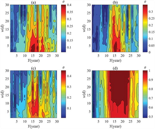
Figure 4(a) and (b) shows that the θ value increased as the Y value changed from 1 to 15 and decreased as the Y value changed from 15 to 30. When the Y value changed from 10 to 20, the θ value was larger compared to when Y was assigned other values. For w, the θ value decreased as w increased when Y was assigned values from 10 to 20. Therefore, when the Y value was 15 and the w value changed from 1 to 5, the θ value was largest. When considering the influence of w on the MASH, the daily variability may not be smoothed out and the seasonal pattern may not emerge if the value is too small. Therefore, in this study, Y = 15 and w = 5 were set as a pair of averaging parameters for MASH of flow and water level at the Xiajiang hydrological station.

Figure 4(c) and (d) shows that the θ value for the water level was larger than the value for flow at the Waizhou hydrological station. For flow, the high θ value was distributed between Y = 10 and Y = 20; there were two maximum points of θ, with w = 10 or w = 20 when Y = 15. Thus, w = 10 or w = 20 with Y = 15 were selected as two pairs of alternative averaging parameters. In other words, both the pair Y = 15 and w = 10 and the pair Y = 15 and w = 20 could serve as averaging parameters. With respect to the water level, a high θ value was distributed in the region where the value of Y changed from 10 to 23. When w > 10, there was a maximum region for the θ value, which was nearly 1 when Y was between 12 and 23. Therefore, Y can range from 12 to 23 and w can range from 10 to 30, as an alternative averaging parameter region. In other words, a pair of averaging parameters can be randomly selected from this range. Considering that the selection range of averaging parameters for water level is broader than the selection range for flow, for convenience, the same pair of Y and w values can be used as averaging parameters. For this study, Y = 15 and w = 10 were established as the pair of averaging parameters for both water level and flow at the Waizhou hydrological station.

4.2 Application of MASH for water level and flow

The previous step established Y = 15 and w = 5 as the pair of averaging parameters of MASH for filtering the daily time series of water level and flow at the Xiajiang hydrological station, while the values Y = 15 and w = 10 were selected for filtering the corresponding data series at the Waizhou hydrological station. The visualization of MASH for the Xiajiang and Waizhou hydrological stations is presented in Figs. 5–7 and Figs. 8–10, respectively.

Figure 5. MASH of daily flow (Y = 15, w = 5) time series at Xiajiang hydrological station.

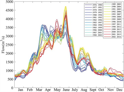
Figure 6. MASH of daily water level (Y = 15, w = 5) time series at Xiajiang hydrological station.

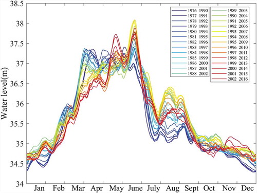
Figure 7. Relationship between water level and flow at Xiajiang hydrological station, with both variables filtered by MASH (Y = 15, w = 5): (a) inter-annual variability and (b) intra-annual variability.

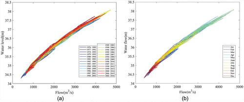
Figure 8. MASH of daily flow (Y = 15, w = 10) time series at Waizhou hydrological station.

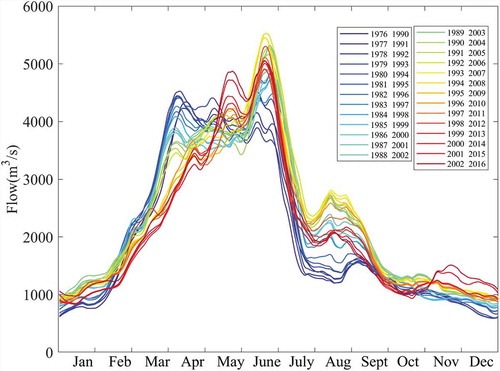
Figure 9. MASH of daily water level (Y = 15, w = 10) time series at Waizhou hydrological station.

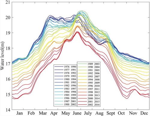
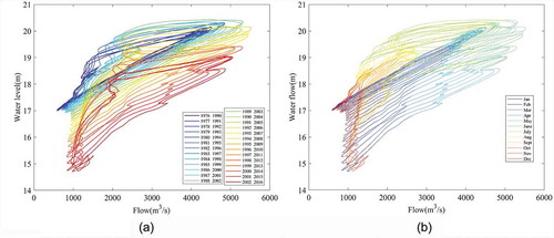
Figure 10. Relationship between water level and flow at Waizhou hydrological station, with both variables filtered by MASH (Y = 15, w = 10): (a) inter-annual variability and (b) intra-annual variability.

Figures 5 and 6 are, respectively, the MASH visual representations for the daily time series of water level and flow at the Xiajiang hydrological station. The length of the original time series was N_y = 41 years (1976–2016); the MASH horizon was N_h = 27 with Y = 15. The older horizons are plotted with blue lines and the more recent horizons are plotted with red lines. For the Xiajiang hydrological station, the water level and flow trends were similar: the smoothed water level and flow values dropped persistently during March and April. There were slight increases in May and June, and fluctuations from July to September. The similarity in water level and flow trends suggests there may not have been a big change in the relationship between these variables in the period 1976–2016.

Figure 7 shows the inter- and intra-annual variability in the relationship between water level and flow at the Xiajiang station. It can be seen from Fig. 7(a) that the different coloured lines closely align and that the related lines do not significantly change from 1976–1990 to 2002–2016. In Fig. 7(b), it may be seen that the maximum flow and water level occurred in the period May–July and the minimum counterparts during the dry season from December to February.

Figures 8 and 9 present, respectively, MASH visual representations for the daily time series of water level and flow at the Waizhou hydrological station. Figure 8 shows a declining trend in the smoothed time series of flow from March to April, with a slight increase from May to June and from November to December. In addition, in August, the smoothed value of flow increases between the horizon 1976–1990 and the horizon 1994–2008 and becomes smaller during 1998–2012. Figure 9 shows that there is a persistent decrease in the smoothed series of water level during the whole period since the 1990s.

Figure 10 shows the visualization of the inter- and intra-annual variability in the relationship between water level and flow at the Waizhou station. The variability trends of the relationship between MASH smoothed water level and flow series can be observed in Fig. 10(a). The blue lines present the relationship of water level and flow from the horizon 1976–1990 to 1981–1995, which are distributed in the upper part of Fig. 10(a). The green and yellow lines, distributed in middle part, present the relationship of water level and flow from horizon 1982–1996 to 1995–2009 and the red lines, distributed in lower part, present the relationship of water level and flow from horizon 1996–2010 to 2002–2016. There is a downward migration from the blue lines to the red lines according to their distribution with time. This means that the more recent horizon smoothed water level values are smaller than the older horizon smoothed values with respect to the same smoothed flow value. The riverbed at the Waizhou station has been lowered by streambed cutting processes since the 1990s and this is evident in the 2002–2016 horizon (see Section 4.4 for further discussion).

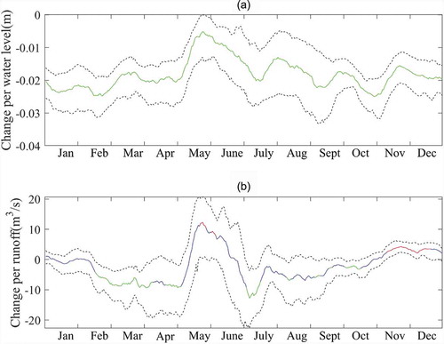
The tendency of changes in the smoothed series of water level and flow was detected using the pre-whitening M-K trend test and Sen’s slope method, with the results presented in Figs. 11 and 12. Figure 11 shows that, for the Xiajiang hydrological station, there were similar trends with respect to changes in the smoothed water level and flow. Significant negative trends in the MASH smoothed series for water level and flow are seen mainly from February to April. There were statistically significant positive trends in mid-May and November. Figure 12(a) shows that, for the Waizhou station, there was a significant decrease in the MASH smoothed time series for the water level throughout the year. As for the MASH smoothed time series for flow, a statistically significant increase is detected from November to mid-December and there was a statistically significant decrease from February until March, in the second half of April and from the end of June until the first half of July (Fig. 12(b)).

Figure 11. Results of the pre-whitening M-K trend test and Sen’s slope method for MASH smoothed (a) water level and (b) flow at Xiajiang hydrological station (confidence level of α = 5%). Green lines represent a significant decrease; red lines represent a significant increase; and blue lines represent a non-significant trend with given confidence level. Dotted lines represent confidence limits of an estimated trend slope at 95%.

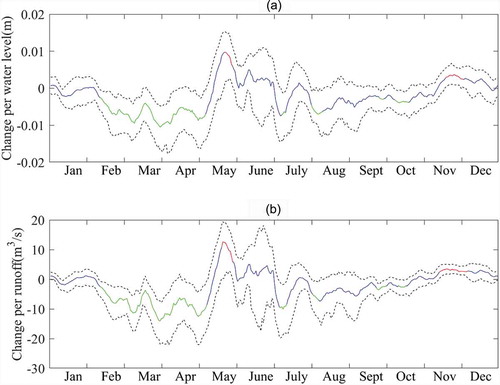
Figure 12. Results of the pre-whitening M-K trend test and Sen’s slope method for MASH smoothed (a) water level and (b) flow at Waizhou hydrological station (confidence level of α = 5%). Green lines represent a significant decrease; red lines represent a significant increase; and blue lines represent a non-significant trend at the given confidence level. The dotted lines represent the confidence limits at an estimated trend slope at 95%.

4.3 Comparison of trend analysis with and without MASH smoothed

The study used the pre-whitening M-K test and Sen’s slope method to analyse the trends in the original water level and flow series and then compared the results with the trend analysis with the smoothed series; the results are presented in Table 1.

Table 1. Results of the pre-whitening M-K trend test and Sen’s slope method applied to the original flow and water level series without MASH smoothing on a monthly basis at a confidence level of α = 0.05. Z is the pre-whitening M-K trend test statistic; Th is the threshold; and β is the Sen slope estimator.

		Flow			Water level
Station	Month	Z	Th	β (m^3s^−1 year^−1)	Z	Th	β (m^3s^−1 year^−1)
Xiajiang	Jan	1.40	1.96	5.50	1.00	1.96	0.01
	Feb	0.03	1.96	0.23	0.24	1.96	0.00
	Mar	–0.44	1.96	–3.68	0.03	1.96	0.00
	Apr	–2.06	1.96	–36.20	–1.74	1.96	–0.03
	May	0.12	1.96	2.02	0.57	1.96	0.01
	Jun	–0.01	1.96	–0.65	0.39	1.96	0.01
	Jul	1.11	1.96	12.22	1.38	1.96	0.02
	Aug	1.09	1.96	8.64	0.86	1.96	0.01
	Sep	0.53	1.96	3.39	0.84	1.96	0.01
	Oct	–0.26	1.96	–1.60	–0.75	1.96	–0.01
	Nov	1.79	1.96	7.50	1.22	1.96	0.01
	Dec	2.64	1.96	9.36	1.79	1.96	0.01
Wazhou	Jan	1.56	1.96	7.20	–2.57	1.96	–0.04
	Feb	0.12	1.96	2.11	–2.39	1.96	–0.05
	Mar	–0.17	1.96	–1.88	–3.27	1.96	–0.06
	Apr	–2.10	1.96	–37.75	–3.16	1.96	–0.06
	May	0.44	1.96	10.28	–2.59	1.96	–0.05
	Jun	0.84	1.96	22.94	–1.92	1.96	–0.04
	Jul	0.86	1.96	16.67	–1.04	1.96	–0.02
	Aug	1.13	1.96	10.83	–1.34	1.96	–0.03
	Sep	0.69	1.96	7.84	–2.53	1.96	–0.05
	Oct	0.10	1.96	0.23	–2.46	1.96	–0.03
	Nov	1.88	1.96	9.98	–2.35	1.96	–0.04
	Dec	2.53	1.96	11.64	–3.22	1.96	–0.05

A statistically negative trend in the flow series is seen at the Xiajiang and Waizhou stations in April and there is a statistically significant increase in December (Table 1). For the water level series, there is no significant trend at the Xiajiang station, but there is a statistically significant decrease in the water level series from January to May and from September to December at the Waizhou station. The absolute trend slope of the water level at the Xiajiang station is approx. 0.01; this is smaller than the absolute slope at the Waizhou station, which is approx. 0.05.

Some differences in trend analyses are seen when comparing the results of trend analysis (Table 1) with the results of trend analysis using MASH (Figs. 5, 6, 8, 9, 11 and 12). With respect to the significance of the statistical trend, there were more significant trends detected in the time series smoothed by MASH compared to the original series. Taking the trend analysis in water level series as an example, Table 1 shows that no statistically significant trends are detected in the periods from June to August, while according to Fig. 12(a), there is a statistically significant decrease in the MASH smoothed water level series from June to August. This is probably because MASH filters and reduces the seasonal and inter-annual variability of the original data series, enhancing the significance of the trends in the water level from June to August (Anghileri et al. 2014, Osuch and Wawrzyniak 2016). As another example, MASH enables us to visualize the inter- and intra-annual variability and facilitates the detection of trends in the data series at finer time scales, e.g. weekly or daily (Osuch and Wawrzyniak 2016). In contrast, the traditional trend analysis method (e.g. M-K test) can quantify the trend analysis of the time series at larger time scales, e.g. monthly and yearly.

Figures 13 and 14 show plots of the relationship between the original flow and water level series at the Xiajiang station and Waizhou stations, respectively. The different colours represent the variability in the relationship between flow and water level series across different years.

Figure 13. Relationship between the original water level and flow series at Xiajiang station.

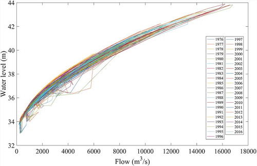
Figure 14. Relationship between the original water level and flow series at Waizhou hydrological station.

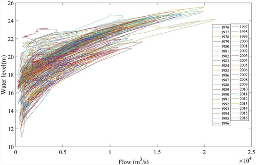
Figure 13 shows a concentration in the distribution of the curves. This means that the relationship between flow and water level series at the Xiajiang station did not significantly change. In contrast, Fig. 14 shows a decentralization trend in the curves, which indicates that the relationship between flow and water level series at the Waizhou station may have changed. However, because the data series were not smoothed by MASH, the trends are not as clear as seen in Fig. 10.

4.4 Discussion on water level variability trends at the Waizhou station

From the trend analysis for water level and flow series in the middle and lower reaches of Ganjiang River, it is shown that there is a statistically significant decrease in the water level at the Waizhou station, while no statistically significant trends are detected in water level and flow at the Xiajiang station. The relationship of water level and flow at the Waizhou station is not as stable as that at the Xiajiang station. In general, the riverbed variability influences the stability of relationship between water level and flow. According to research carried out by Zhang et al. (2011) and Chen et al. (2012), human activities, especially reservoir construction upstream and large-scale sand mining in the lower reaches of the Ganjiang River, have reduced the river sediment load and strengthened the riverbed cutting-down processes since the 1990s.

The construction of reservoirs upstream did not change the inter-annual trends of flow at the Waizhou station but decreased the sediment load in the lower reaches significantly (Zhang et al. 2010). For example, Wan’an Reservoir is the largest reservoir in the Ganjiang River. The basin area above Wan’an Reservoir is about 36 900 km², accounting for 90% of the upper basin area (Du et al. 2016). According to the study of Wen et al. (2019), the mean sediment load into Wan’an Reservoir in the period 1990–2014 was 4.6 × 10⁶ t/year, while the mean value out of Wan’an Reservoir was 3.2 × 10⁶ t/year. This indicates that the sedimentation of Wan’an Reservoir played an important role in the sediment load reduction (Wen et al. 2019).

Table 2 shows the sediment load variability at the Waizhou station during the periods from 1971–1980 to 2001–2010 (Chen et al. 2012, Shi and Shi 2016).

Table 2. Statistical table of sediment during different periods at Waizhou station. Data source: Chen et al. (2012) and Shi and Shi (2016).

Period	Mean annual discharge (10^9 m^3)	Mean annual sediment load (10^6 t)	Mean annual sediment concentration (kg/m^3)
1971–1980	67.2	10.6	0.16
1981–1990	65.3	10.0	0.15
1991–2000	772.3	5.7	0.07
2001–2010	66.7	3.4	0.05

As may be observed from Table 2, the mean annual sediment load at the Waizhou station during the period 1971–1990 was about 10 × 10⁶ t, then it reduced to 5.7 × 10⁶ t during the period 1991–2000 and decreased to 3.4 × 10⁶ t during the periods 2001–2010. However, the mean annual sand mining at the Waizhou station has been over 20 × 10⁶ t since the 2000s, much more than the mean annual sediment load. This may strengthen the riverbed cutting-down processes and make the riverbed lower. In addition, because of the operation of the Three Gorges Reservoir and other factors, the mean annual water level of Poyang Lake has decreased by 0.02 m since the 1980s. This may also increase the flow surface gradient and flow velocity, strengthening the erosion of the riverbed (Chen et al. 2012).

5 Summary and conclusions

This study investigated daily time series trends for flow and water levels from the beginning of 1976 to the end of 2016 at two hydrological stations (Waizhou and Xiajiang) in the middle and lower reaches of the Ganjiang River in China. The pre-whitening Mann-Kendall trend test was used to detect the inter-annual variability in the flow and water level and MASH, combined with Sen’s slope method, was applied to quantifiably analyse the inter- and intra-annual trends of the flow and water level series. There were four main conclusions from the study.

First, MASH (Moving Average over Shifting Horizon) is a novel EDA (exploratory data analysis) method that simultaneously analyses the inter- and intra-annual trends of the time series. It uses two parameters to smooth the original series: the number of days, w, and years, Y. However, there is no general rule for selecting these parameters, limiting the use of this type of technique. In this study, the SCRM (significant change rate) method was proposed to help select the MASH averaging parameters w and Y. SCRM defines the significant change rate θ and plots a contour map to establish a relationship between θ and averaging parameters. In SCRM, the value of θ is assumed to be certain if the value of Y and w is determined. Meanwhile, θ is an index that can evaluate the result of the MASH trend analysis. The larger the θ value, the clearer the MASH trend result is. Therefore, the corresponding Y and w of the largest θ were selected as the averaging parameters. Based on the SCRM results, the averaging parameters were selected for MASH for both the time series of water level and flow at both stations: Y = 15 and w = 5 for the Xiajiang hydrological station; and Y = 15 and w = 10 for the Waizhou hydrological station. The SCRM can narrow the scope of choice for the MASH averaging parameters, reduce the randomness of parameter selection and facilitate parameter selection.

Second, based on the SCRM results, the study applied MASH to filter the daily time series of water level and flow at both stations. Variable trends were quantified using the pre-whitening M-K trend test and Sen’s slope method. The results revealed that, for the smoothed flow and water level series at the Xiajiang station, there was a statistically significant decrease in the period from February to April and a significant increase detected in mid-May and November. For the smoothed flow series at the Waizhou station, the statistically negative trends were mainly seen from February until March, during the second half of April and from the end of June until the first half of July. The trend was significantly positive from November to mid-December. For water level at the Waizhou station, there was a significant decrease in the MASH smoothed series of water level throughout the year after the 2000s. In addition, the relationship between the MASH smoothed water level and flow at the Waizhou hydrological station changed significantly.

Third, the study compared the trends for the original flow and water level series against the analysis of corresponding data series smoothed using MASH. MASH enabled the visualization of inter- and intra-annual trends, increased the visibility of the data series and quantified the trends combined with traditional mathematical methods, such as the M-K test and Sen’s slope method.

Finally, this study discussed the causes of the statistically significant water-level decrease and instability in the relationship of water level and flow at the Waizhou station. The decreasing trends of water level are related to the sediment load reduction and human activities, such as upstream reservoir construction and large-scale sand mining, which played an important role in reducing the sediment load.

Acknowledgements

The authors acknowledge the Jiangxi Provincial Institute of Water Sciences for providing the data for this study.

Disclosure statement

No potential conflict of interest was reported by the authors.

Additional information

Funding

This study was financially supported by the National Natural Science Foundation of China [Grant no. 51479140], the National Key R&D Program of China [Grant no. 2016YFC0401306] and the Science and Technology Project of Water Resources Department of Jiangxi Province [Grant no. KT201704].

References

- Allan, R.P. and Soden, B.J., 2008. Atmospheric warming and the amplification of precipitation extremes. Science, 321 (5895), 1481–1484. doi:10.1126/science.1160787
- Alrajoula, M.T., et al., 2016. Hydrological, socio-economic and reservoir alterations of Er Roseires Dam in Sudan. Science of Total Environment, 566–567, 938–948. doi:10.1016/j.scitotenv.2016.05.029
- Anghileri, D., Pianosi, F., and Soncini-sessa, R., 2014. Trend detection in seasonal data: from hydrology to water resources. Journal of Hydrology, 511 (4), 171–179. doi:10.1016/j.jhydrol.2014.01.022
- Benjamin, L. and Vankrik, R.W., 1999. Assessing instream flows and reservoir operations of an Eastern Idaho River. Journal of the American Water Resources Association, 35, 899–909. doi:10.1111/j.1752-1688.1999.tb04183.x
- Cardwell, H., Jager, H.I., and Sale, M.J., 1996. Designing instream flows to satisfy fish and human water needs. Journal of Water Resources Planning and Management, 122, 356–363. doi:10.1061/(ASCE)0733-9496(1996)122:5(356)
- Chen, J., et al., 2012. Runoff-sediment characteristics and riverbed evolution of Ganjiang River sink. Advances in Science and Technology of Water Resources, 32 (3), 1–5 ( in Chinese).
- Chen, J., Liu, H., and Lv, T., 2016. Analysis of low water level variation and cause for Ganjiang trial channel. Water Resources and Power, 34 (10), 28–31. (in Chinese).
- Dietz, E.J. and Killeen, T.J., 1981. A Nonparametric multivariate test for monotone trend with pharmaceutical applications. Publications of the American Statistical Association, 76, 169–174.
- Du, J., et al., 2016. Evaluating functions of reservoirs’ storage capacities and locations on daily peak attenuation for Ganjiang River Basin using Xinanjiang model. Chinese Geographical Science, 26 (6), 789–802. doi:10.1007/s11769-016-0838-6
- Fu, K.D., He, D.M., and Lu, X.X., 2008. Sedimentation in the Manwan Reservoir in the Upper Mekong and its downstream impacts. Quaternary International, 186 (1), 91–99. doi:10.1016/j.quaint.2007.09.041
- Gocic, M. and Trajkovic, S., 2013. Analysis of changes in meteorological variables using Mann-Kendall and Sen’s slope estimator statistical tests in Serbia. Global and Planetary Change, 100, 172–182. doi:10.1016/j.gloplacha.2012.10.014
- Guo, L., et al., 2019. Assessing impacts of climate change and human activities on streamflow and sediment discharge in the Ganjiang River Basin (1964–2013). Water, 11 (8), 1679. doi:10.3390/w11081679
- Hu, Q., et al., 2007. Interactions of the Yangtze River flow and hydrologic processes of the Poyang Lake, China. Journal of Hydrology, 347 (1–2), 90–100. doi:10.1016/j.jhydrol.2007.09.005
- Huang, Y., et al., 2019. Assessment of hydrological changes and their influence on the aquatic ecology over the last 58 years in Ganjiang Basin, China. Sustainability, 11, 4882. doi:10.3390/su11184882
- Jiang, J. and Huang, Q., 1997. A study of the impact of the three gorges project on the water level of Poyang Lake. Journal of Natural Resources, 3, 24–29 ( in Chinese).
- Kendall, M.G., 1975. Rank correlation methods. Charles Griffin: London.
- Li, D., et al., 2017. Observed changes in flow regimes in the mekong river basin. Journal of Hydrology, 551, 217–232. doi:10.1016/j.jhydrol.2017.05.061
- Li, J., et al., 2015. Future joint probability behaviors of precipitation extremes across China: spatiotemporal patterns and implications for flood and drought hazards. Global and Planetary Change, 124, 107–122. doi:10.1016/j.gloplacha.2014.11.012
- Li, Y. and Zhang, Q., 2018. Historical and predicted variations of baseflow in china’s Poyang Lake catchment. River Research and Applications, 34 (10), 1286–1297. doi:10.1002/rra.3379
- Liu, G.H., et al., 2016. Quantitative estimation of runoff changes in Ganjiang River, Lake Poyang Basin under climate change and anthropogenic impacts. Journal of Lake Sciences, 28 (3), 682–690. doi:10.18307/2016.0326
- Magilligan, F.J., et al., 2016. Immediate changes in stream channel geomorphology, aquatic habitat, and fish assemblages following dam removal in a small upland catchment. Geomorphology, 252, 158–170. doi:10.1016/j.geomorph.2015.07.027
- Mann, H., 1945. Nonparametric tests against trend. Econometrica, 13 (3), 245–259. doi:10.2307/1907187
- Oguntunde, P., Abiodun, B., and Lischeid, G., 2011. Rainfall trends in Nigeria, 1901–2000. Journal of Hydrology, 411 (3–4), 207–218. doi:10.1016/j.jhydrol.2011.09.037
- Osuch, M. and Wawrzyniak, T., 2016. Inter- and intra-annual changes in air temperature and precipitation in western Spitsbergen. International Journal of Climatology, 37, 3082–3097. doi:10.1002/joc.4901
- Osuch, M. and Wawrzyniak, T., 2017. Variations and changes in snow depth at meteorological stations Barentsburg and Hornsund (Spitsbergen). Annals of Glaciology, 58 (75pt1), 11–20. doi:10.1017/aog.2017.20
- Poff, N.L., et al., 1997. The natural flow regime. BioScience, 47 (11), 769–784. doi:10.2307/1313099
- Richter, B.D., et al., 1996. A method for assessing hydrologic alteration within ecosystems. Conservation Biology, 10 (4), 1163–1174. doi:10.1046/j.1523-1739.1996.10041163.x
- Rougé, C., Ge, Y., and Cai, X., 2013. Detecting gradual and abrupt changes in hydrological records. Advances in Water Resources, 53, 33–44. doi:10.1016/j.advwatres.2012.09.008
- Sen, P.K., 1968. Estimates of the regression coefficient based on Kendall’s tau. Journal of the American Statistical Association, 63 (324), 1379–1389. doi:10.1080/01621459.1968.10480934
- Shankman, D., Keim, B.D., and Song, J., 2010. Flood frequency in china’s poyang lake region: trends and teleconnections. International Journal of Climatology, 26 (9), 1255–1266. doi:10.1002/joc.1307
- Shi, M. and Shi, X., 2016. Influence and analysis of the water level decreasing continuously in the dry season in the lower reaches of the Ganjiang River. China Flood and Drought Management, 26 (4), 55–58+96 ( in Chinese).
- Sonali, P. and Kumar, D.N., 2013. Review of trend detection methods and their application to detect temperature changes in India. Journal of Hydrology, 476, 212–227. doi:10.1016/j.jhydrol.2012.10.034
- Song, X., et al., 2018. Combined effect of danjiangkou reservoir and cascade reservoirs on hydrologic regime downstream. Journal of Hydrologic Engineering, 23 (6), 05018008. doi:10.1061/(ASCE)HE.1943-5584.0001660
- Tu, X., et al., 2015. Intra-annual distribution of streamflow and individual impacts of climate change and human activities in the Dongjiang River basin, China. Water Resources Management, 29 (8), 2677–2695. doi:10.1007/s11269-015-0963-5
- Von Storch, H., 1995. Analysis of climate variability. Berlin: Springer-Verlag.
- Walling, D.E., 1983. The sediment delivery problem. Journal of Hydrology, 65 (1–3), 0–237. doi:10.1016/0022-1694(83)90217-2
- Wang, G., Wu, B., and Wang, Z.Y., 2005. Sedimentation problems and management strategies of Sanmenxia Reservoir, Yellow River, China. Water Resources Research, 41 (9), 477–487. doi:10.1029/2004WR003919
- Wang, R., et al., 2017. Length-weight relationships of nine fish species from the upper reach of the gan river, a tributary of the yangtze river in China. Journal of Applied Ichthyology, 34 (1), 230–232. doi:10.1111/jai.13549
- Wang, Z., et al., 2019. Spatial and temporal characteristics of reference evapotranspiration and its climatic driving factors over China from 1979–2015. Agricultural Water Management, 213, 1096–1108. doi:10.1016/j.agwat.2018.12.006
- Wen, T., et al., 2019. Effects of climate variability and human activities on suspended sediment load in the Ganjiang River Basin, China. Journal of Hydrologic Engineering, 24 (11), 05019029. doi:10.1061/(ASCE)HE.1943-5584.0001859
- Yang, T., et al., 2008. A spatial assessment of hydrologic alteration caused by dam construction in the middle and lower Yellow River, China. Hydrological Processes, 22 (18), 3829–3843. doi:10.1002/hyp.6993
- Yang, Y., et al., 2019. Impacts of groundwater depth on regional scale soil gleyization under changing climate in the Poyang Lake Basin, China. Journal of Hydrology, 568, 501–516. doi:10.1016/j.jhydrol.2018.11.006
- Yu, S., Yang, J., and Liu, G., 2014. Impact assessment of three Gorges Dam’s impoundment on river dynamics in the north branch of Yangtze River estuary, China. Environmental Earth Sciences, 72 (2), 499–509. doi:10.1007/s12665-013-2971-1
- Yue, S. and Wang, C.Y., 2002. Applicability of prewhitening to eliminate the influence of serial correlation on the Mann-Kendall test. Water Resources Research, 38 (6), 4–1–4–7. doi:10.1029/2001WR000861
- Zhang, D., et al., 2017a. Copula-based probability of concurrent hydrological drought in the Poyang Lake-catchment-river system (China) from 1960 to 2013. Journal of Hydrology, 553, 773–784. doi:10.1016/j.jhydrol.2017.08.046
- Zhang, Q., Chen, X., and Chen, Y., 2010. Spatio-temporal patterns of sediment and runoff changes in the Poyang Lake basin and underlying causes. Acta Geographica Sinica, 65 (7), 828–840 ( in Chinese).
- Zhang, Q., et al., 2016. Evaluation of impacts of climate change and human activities on streamflow in the poyang lake basin, China. Hydrological Processes, 30, 2562–2576. doi:10.1002/hyp.10814
- Zhang, Q., et al., 2011. Spatio-temporal patterns of hydrological processes and their responses to human activities in the Poyang Lake basin, China. Hydrological Sciences Journal, 56 (2), 305–318. doi:10.1080/02626667.2011.553615
- Zhang, Q., et al., 2014. Topography-based spatial patterns of precipitation extremes in the Poyang lake basin, china: changing properties and causes. Journal of Hydrology, 512, 229–239. doi:10.1016/j.jhydrol.2014.03.010
- Zhang, X., et al., 2019. A hierarchical Bayesian model for decomposing the impacts of human activities and climate change on water resources in China. Science of the Total Environment, 665, 836–847. doi:10.1016/j.scitotenv.2019.02.189
- Zhang, Y., et al., 2017b. Flash droughts in a typical humid and subtropical basin: a case study in the Gan River basin, China. Journal of Hydrology, 551, 162–176. doi:10.1016/j.jhydrol.2017.05.044
- Zhang, Z., et al., 2015. Examining the influence of river–lake interaction on the drought and water resources in the Poyang Lake basin. Journal of Hydrology, 522, 510–521. doi:10.1016/j.jhydrol.2015.01.008