Assessing the impacts of land cover and climate on runoff and sediment yield of a river basin

ABSTRACT

This study investigated the impacts of changes in land cover and climate on runoff and sediment yield in a river basin in India. Land Change Modeler was used to derive the future land cover and its changes using the Sankey diagram approach. The future climatic parameters were derived from five general circulation models for two emission scenarios with representative concentration pathways (RCPs) 4.5 and 8.5. The land cover and climate change impacts on runoff and sediment yield were estimated using SWAT model. The results show important changes in land cover and indicate that urban and agricultural areas strongly influence the runoff and sediment yield. Among the land cover and climate change impacts, climate has more predominant (70%–95%) impact. Runoff and sediment yield are likely to decrease in both RCP scenarios in the future period. The impacts of land cover changes are more prominent on sediment yield than runoff.

KEYWORDS:

• land cover
• Land Change Modeler
• Sankey diagram
• climate change
• SWAT model
• runoff
• sediment yield

Editor A. Fiori; Associate editor R. Singh

1 Introduction

Extreme land cover and climate changes have been reported in many parts of the world in the last few decades and these have been expected to increase in the future (IPCC 2013). Land cover and climate changes are the two major factors affecting the changing hydrological processes at a river basin scale (Li et al. 2009, Wada et al. 2011). Generally, the change in land cover alters the hydrological cycle by changing the evapotranspiration (ET), infiltration rate (Rientjes et al. 2011), soil moisture, base flow (Wang et al. 2006), and runoff (Yan et al. 2013, Sinha and Eldho 2018); while, climate variability may alter the rainfall, humidity (Wang et al. 2008), routing time, peak flow, and runoff volume (Prowse et al. 2006). Moreover, change in climate may also alter the land use pattern and with increase in temperature may reduce the crops. Further, a warmer and drier climate in the coming decades will increase the likelihood of drought, shift cropping pattern and farming methods, which may affect surface runoff and soil erosion of the catchment considered. Hence, understanding the effects of changes in land cover and climate is critical for the water resource management at the river basin scale. In India, the rapid growth in population and socioeconomic development and lack of sufficient water resources may considerably increase the water scarcity (Wagner et al. 2016). In addition, recent studies have highlighted that water resources have been depleted in various regions of India (Mishra et al. 2007, Garg et al. 2013, Wagner et al. 2013). Nevertheless, the combined effect of changes in land cover and climate on hydrology in developing countries, such as India, is largely unknown. Thus, there is a need of integrated modelling approach to study the individual and combined effects of future climate and LULC change on hydrology using a physically distributed hydrological model, which can provide reasonable information on the spatio-temporal water resource management and land use planning strategies.

In this context, previous studies have shown that land cover and climate changes can have prominent effects on runoff (Tomer and Schilling 2009, Wilson and Weng 2011, Kim et al. 2013, Islam et al. 2014, Chawla and Mujumdar 2015, Farjad et al. 2017) and sediment yield (Jiongxin 2003, Syvitski et al. 2005, Bussi et al. 2016, Zuo et al. 2016, Op de Hipt et al. 2018, 2019). For instance, Chawla and Mujumdar (2015) estimated the impacts of land use (historical) and climate change on upper Ganga river basin using VIC model and found climate change has more effect on streamflow in comparison to land use. Farjad et al. (2017) investigated impacts of future land cover and climate change using MIKE SHE/MIKE 11 model on streamflow in the Elbow river basin in Southern Alberta, Canada which found rise in streamflow and subsequently increase the vulnerability to spring flood in the basin. Zuo et al. (2016) investigated runoff and sediment yield in the Loess Plateau of China due to land use (historical) and climate change using SWAT model and found that both have greater impact on the reduction of annual runoff and sediment yield in the basin. Op de Hipt et al. (2019) studied the Dano catchment in the south-western Burkina Faso, West Africa using SHETRAN model to investigate the land cover and climate change on soil erosion and observed that climate change has larger impact on discharge and sediment yield. In another study, Op de Hipt et al. (2018) investigated the impacts of climate change on same basin and found increase of future discharge and soil erosion in representative concentration pathway (RCP) emissions scenarios RCP4.5 and RCP8.5. Other studies have investigated the effects of future climate change on the hydrology, without considering the future land cover change (Zhang et al. 2007, Abbaspour et al. 2009, Li et al. 2009, Bekele and Knapp 2010, Chawla and Mujumdar 2015, Zuo et al. 2016). Similarly, some studies have focused on future land cover changes in one area only, without incorporating any hydrological modeling (Petit et al. 2001, Zhang and Li 2005, Rounsevell et al. 2006). To date, a limited number of studies have examined the combined effects of land cover and climate changes considering the future impacts on a river basin scale in different regions (Gebremicael et al. 2013, Khoi and Suetsugi 2014, Zuo et al. 2016, Yang et al. 2019). From the above studies, it has been noticed that analysis of different land cover and climate change of the past, present and future on surface runoff and sediment yield is lacking in developing country like India at sub-basin scale where agriculturally based economy is dominant in the humid tropic region.

The methods usually applied for assessments of the impacts of changes in land cover and climate on hydrological process include: (i) experimental paired catchment method, (ii) statistical technique (time series analysis), (iii) distributed hydrological modeling (Li et al. 2009), and (iv) conceptual models (Chawla and Mujumdar 2015). The experimental approach is the most efficient method and is traditionally used for small catchments; however, it is cost-intensive (Zuo et al. 2016) and not applicable to two similar and large-sized catchments (Lørup et al. 1998). The statistical technique is easier to implement; however, this method only analyzes the hydrological effects on the environment due to lack of physical connection (Li et al. 2009, Zuo et al. 2016). The conceptual model requires few parameters to simulate the hydrological process of catchment, but it mainly lacks a correct representation of the whole catchment (Chawla and Mujumdar 2015). Among these, the distributed hydrological model is the most suitable tool for impact assessment (Mango et al. 2011, Wang et al. 2012) because it can relate physically observed parameters directly to the model parameters. In addition, it relates physically based equation at HRUs (Hydrological Response Units) level separately, and the results are spatially aggregated for each sub-basin (Lenhart et al. 2005). The leading hydrological models applied for computing the effects of land cover and climate change on runoff and sediment yield on the river basin scale include: Soil and Water Assessment Tool (SWAT), SHETRAN, Water Erosion Prediction Project, and Hydrological Simulation Program-Fortran etc. Among these, SWAT is the most commonly used tool (Kim et al. 2013, Jordan et al. 2014).

In this study, the semi-distributed hydrological model SWAT is used for computing the impacts of land cover and climate change on runoff and sediment yield on a river sub-basin scale. Here, the Valapattanam River Basin (VRB) is selected as a case study which shows a decrease in trend of precipitation (approximately by 584 mm over the last 20 years) which has greatly affected the hydrology and water resource of the area. It has affected not only the water demand and agriculture system but also runoff and sediment yield. Plantation, agriculture, and unorganized urban development, which require adequate amounts of water, cover the major extent of the basin. Moreover, being a medium river basin located in a highly mountainous region (0–1566-m elevation), it has scarcity of surface water and groundwater availability. Thus, the VRB may encounter serious problems due to changes in climate and land cover on the hydrology in the future. Therefore, this study is aimed to (i) identify the land cover change during 1972–2030, (ii) assess the impacts due to land cover change on runoff and sediment yield, (iii) compute the impacts of climate change on runoff and sediment yield, and (iv) assess the combined effects of land cover and climate changes on runoff and sediment yield in the VRB.

2 Study area and data description

2.1 Study area

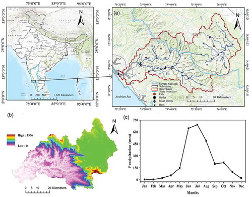
The Western Ghats region of India is one of the global biological hotspots due to the biodiversity and presence of a variety of species (Myers et al. 2000). This region expands along the west coast of India between 08°19′08″−21°16′24″N and 72°56′24″−78°19′40″E, with a north-to-south distance of 1490 km, covering a total area of 136,800 km² (CEPF 2007). In the Western Ghats region, the VRB is situated between 11°47″–12°26″N and 75°14″–76°09″E, with elevation in the range of 0 − 1566 m (Fig. 1(b)), with a total length of approximately 117 km (source-to-outlet), and drainage area of 2517.22 km² (Fig. 1). As per the 2014 land cover analysis, the basin is mainly covered by evergreen and mixed forests (57.1%), followed by plantation (20.6%) and agriculture (16.9%). Two types of crops (paddy and pulse) are typically grown in the area during the two seasons of kharif (July–November) and rabi (December–March) respectively. There is a small dam on the upstream side which is used for irrigation water supply in the river basin. According to the census data of Gov. of India (http://censusindia.gov.in/), the average population density has increased from 759 to 852 per km² in the downstream area (Kannur districts) and 119 to 135 per km² in the upstream (Kodagu districts) during 1991 to 2011 respectively. The majority of the population of river basin area is dependent directly or indirectly on the agriculture for their livelihood. The annual precipitation of the VRB in the Western Ghats has been decreasing over the last 20 years, from 2794 mm in 1990–2000 to 2210 mm in 2001–2010. The average annual precipitation is 2471.6 mm (based on 1971 to 2010 data) and most of the precipitation (approximately 82%) occurs from June to September monsoon months (Fig. 1(c)). The average minimum and maximum temperatures of the basin are 19.63°C and 29.12°C, respectively. As per the soil map which was procured from Food and Agricultural Organization (Table 1) of the VRB, sandy clay loam (approximately 45%) and clay loam (approximately 55%) are predominant. The land cover classes include forest (evergreen and mixed), agriculture (paddy and pulses), grassland, plantation, water, and urban area. Here, the river basin was divided into 38 sub-basins for hydrological parameter studies (Fig. 1).

Table 1. Input data and GCMs from the CORDEX project used in the present study.

Input data	Resolution	Source
Cartosat digital elevation model (DEM)	30 m	National Remote Sensing Centre (http://www.nrsc.gov.in/)
Land use map	30 m	Landsat imageries (http://earthexplorer.usgs.gov/)
Soil type map	1000 m	Food and Agriculture Organization of the United Nation (FAO)
Meteorological data (rainfall and min-max temperature)	0.25º (daily)	Indian Meteorological Department (IMD)
Meteorological data (solar radiation, relative humidity and wind velocity)	0.25º (daily)	https://globalweather.tamu.edu
Observed Hydrological data (streamflow and sediment yields)	Daily	Central Water Commission (http://www.india-wris.nrsc.gov.in/)
GCMs used from the CORDEX project
Modeling center experiment name	Driving GCM (abbreviation)	Institution
Commonwealth Scientific and Industrial Research Organization (CSIRO) Australia – CCAM	ACCESS1.0 (ACC)	CSIRO
	CCSM4 (CCS)	National Centre for Atmospheric Research
	CNRM-CM5 (CNR)	Centre National de Recherches Météorologiques
	MPI-ESM-LR (MPI)	Max Plank Institute for Meteorology (MPI-M)
	NorESM1-M(NOR)	Norwegian Climate Centre

Figure 1. (a) Location map and sub-basins of the study area, (b) digital elevation model and (c) average monthly precipitation of the study area.

2.2 Data used

The digital elevation model, soil, land cover, and meteorological data were used as inputs for simulation of the model in this study. The hydrological data such as observed runoff (Q_obs) and sediment yield (SY_obs) were collected from a gauging location at Perumannu for the years 1986–2010 at daily time scale from the Central Water Commission of India. The relevant details of the input data, resolutions, and sources are listed in Table 1.

Future dynamical downscaled climate variables, namely precipitation and temperature (minimum and maximum), were procured from Coordinated Regional Downscaled Experiment South Asia group (http://cccr.tropmet.res.in/cordex/files/downloads.jsp) for five Coupled Model Inter comparison Project 5 (CMIP5) using general circulation model (GCM) simulation in daily time steps (Table 1). All GCMs contained essential variables corresponding to historic and projected climate data determined using RCP4.5 and RCP8.5 emissions scenarios.

3 Methodology

3.1 SWAT modelling

For runoff and sediment yield simulation, a semi-distributed, open-source, physically based hydrological model SWAT (version 2012), interfaced with ArcGIS, was used. The SWAT model was initially developed for simulating ungauged river basins (Arnold et al. 1998), particularly in cases of limited data availability (Ndomba et al. 2008). It can also be efficiently used for assessing the land cover and climate change effects on runoff and sediment yield (Khoi and Suetsugi 2014, Zuo et al. 2016). The SWAT model involves large calibration uncertainty resulting from the measured or observed data. Because of its simplicity and effectiveness, the use of SWAT-Calibration and Uncertainty Program with Sequential and Uncertainty Fitting (SUFI-2) algorithm is preferred (Abbaspour et al. 2007, Arnold et al. 2012, Fukhrudin et al. 2013, Azari et al. 2016). The SWAT model illustrates the connection among inputs (such as precipitation and temperature), the system conditions (such as land use, soil, and slope), and outputs (such as runoff and sediment yield). In SWAT model, the river catchment is divided into sub-basins and further subdivided them into hydrological response units (HRUs) based on land use, soil, and slope uniqueness. The simulated processes involve surface runoff, infiltration, base flow, lateral flow, plant uptake, ET, and percolation into deep and shallow aquifers. The soil conservation service (SCS) curve number (CN) method (USDA, 1972) is used for computing surface runoff because it can consider daily input data (Arnold et al. 1998) on the basis of the soil hydrological groups, antecedent soil moisture, and land cover characteristics. The Modified Universal Soil Loss Equation (MUSLE) (Williams 1975) is used for analyzing the soil erosion because it considers runoff factors for the calculation of sediment yield in every sub-basin and at the basin outlet. Neitsch et al. (2011) described additional technical details of SWAT model regarding surface runoff and sediment yield. Table 2 shows the important parameters related to surface runoff and sediment yield in the SWAT model.

Table 2. SWAT parameters, description range and its units.

S.N.	Parameters of SWAT Model	Description	Lower – Upper range	Hydrological process	Units
1	CN2	Initial SCS CN II Value	35 − 98	Runoff
2	SOL_AWC	Available water capacity of the soil layer	0 − 1	Soil	mm/mm
3	ESCO	Soil evaporation compensation factors	0 − 1	Evaporation
4	EPCO	Plant uptake compensation factor	0 − 1	Evaporation
5	RCHRG_DP	Deep aquifer percolation factor	0 − 1	Groundwater
6	SUR_LAG	Surface runoff lag time	0.05 − 24	Runoff	d
7	ALPHA_BF	Base flow alpha factor	0 − 1	Groundwater
8	USLE_P	USLE equation support practice factor	0 − 1	Soil
9	USLE_K	USLE soil erodibility factor	0 − 0.65	Soil
10	GWQMN	Threshold depth of water in the shallow aquifer required for return flow	0 − 3000	Groundwater	mm
11	GW_DELAY	Groundwater delay	0 − 500	Groundwater	d
12	GW_REVAP	Groundwater “revap” coefficient	0.02 − 0.2	Groundwater
13	LAT_SED	Sedimentation concentration in lateral flow and groundwater flow	0 − 5000	Sediment	mg/L
14	HRU_SLP	Average slope steepness	0 − 1	Geomorphology	m/m
15	SLSUBBSN	Average slope length	10 − 150	Geomorphology	m
16	SPCON	Linear parameter for calculating the maximum amount of sediment load that can be re-entered during channel sediment routing	0.0001 − 0.1	Sediment
17	CH_ERODMO	Channel erodibility factor	0 − 1	Channel
18	CH_N2	Manning’s “n” value for the main channel	−0.01 − 0.3	Channel
19	BLAI	Max leaf area index	0.5 − 10	Crop
20	SOL_Z	Depth from soil surface to bottom of layer	0 − 3000	Soil	mm
21	BIOMIX	Biological mixing efficiency	0 − 1	Management
22	SOL_ALB	Moist soil albedo	0 − 0.25	Evaporation
23	CH_COV1	Channel cover factor	−0.05 − 0.6	Channel	m/m
24	SPEXP	Exponent parameter for calculating sediment re-entrained in channel sediment routing	1 − 1.5	Sediment
25	PRF	Peak rate adjustment factor for sediment routing in the main channel	0 − 2	Channel
26	ADJ_PKR	Peak rate adjustment factor for sediment routing in the subbasin (tributary channels)	0.5 − 2	Channel
27	CH_K2	Effective hydraulic conductivity in main channel alluvium	−0.1 − 500	Channel	mm/h
28	CH_S2	Average slope of main channel	0.001 − 10	Channel	m/m

3.2 Pre-processing of Landsat image and projection of future land cover map

Landsat images were procured for 1972, 1979, 1988, 2000, and 2014 for determining changes in land cover. The Landsat images were corrected for atmospheric interference by using the dark-object subtraction method before classification (Jensen 2005) and topographic correction. All the images used in this study were free of cloud and collected in the post-monsoon season (October to January). The supervised maximum likelihood technique was used for image classification due to its strength (Lu and Weng 2007). Mainly seven land use classes such as forest, mixed forest, plantation, agriculture, grassland, urban, and water bodies were classified. The overall accuracy and kappa coefficient (κ) in the ranges of 83%–94% and 0.79–0.87, respectively, are normally acceptable. The details of the classified images and their changes are presented in Section 4.1.

For determining the effects of future changes in land cover on runoff and sediment yield, the future land cover for 2030 were projected. The multiperceptron neural system build on Markov transition matrix technique incorporated in Land Change Modeler (LCM) of Idrisi’s model was used for developing the 2030 land cover map for the VRB. The equation below represents the Markov transition matrix (m × n) (Weng 2002):

(1) $X_{ij}^{\ast }=\frac{X_{ij}-\begin{array}{c}Min\left({\mathrm{X}}_{\mathrm{i}\mathrm{j}}\right)\\ j=1,2,\dots q\end{array}}{\begin{array}{c}Max\left({\mathrm{X}}_{\mathrm{i}\mathrm{j}}\right)\\ j=1,2,\dots q\end{array}-\begin{array}{c}Min\left({\mathrm{X}}_{\mathrm{i}\mathrm{j}}\right)\\ j=1,2,\dots q\end{array}}\mathrm{f}\mathrm{o}\mathrm{r}\mathrm{j}=1,2,\dots .\mathrm{q}$(1)

where P_ij is the transition probability of state i to j for different land use classes.

The cellular automata (CA) constitute the physical spaces categorized by cells, in which the CA operations occur (Barredo et al. 2003, Sinha and Eldho 2018), as well as the neighbourhood that surrounds these cells. The rules of transition defining the performance of the CA in the time-based space, under all mechanism exists (Li and Yeh 2000) and can be represented as;

(2) $\xi$(2)

where S is the set of all possible conditions of CA, N is the neighbourhood of all cells, and f is the transition function that defines the change from t to t + 1.

To understand the spatiotemporal evolution processes and conversion of various land cover classes that deals with the Markov transition matrix, the LCM model this model combines the Markov chain and CA. The CA fundamentally deals physical structures of the model by using mathematical processes, in which space and time are independent. During the projection of future land cover maps, various drivers of land cover change such as population growth, economic development, infrastructure growth, agricultural development etc. were used. These drivers determined the evidence probability of land cover changes between 2000 and 2014, including changes in the urban area, water bodies, road distance, the basin slope, land cover, demographic, and socioeconomic development dataset. The demographic and socio-economic development dataset were procured from the census of India¹ and statics of socio-economic development of India.² These datasets cover all districts present in the river basin and include demographic, social, and economic statistics. The projection abilities of all the drivers of LULC change were verified during the projection of the future image.

The whole mechanism was applied for future land cover projection in two steps. At first, the land cover map of 2014 was projected with the help of the classified land cover maps of 1988 and 2000 to confirm the multiperceptron neural network in the LCM, recognize the major factors causing land cover changes, and examine the prediction of land cover from the model (Sinha and Eldho 2018). The land cover images of 1988 and 2000 were used as the LCM calibration data. The classified land cover image of 2014 was utilized to analyze the simulated land cover map of 2014. The neural network was retrained continuously till the projected and the classified land cover map of 2014 was matched. After this process, the classified maps of 2000 and 2014 were used to simulate the land cover map of 2030. This step enabled the prediction of important transitions likely to occur in the VRB between 2014 and 2030.

3.3 GCM climate data and pre-processing

Generally, GCMs outputs cannot be recommended for direct use for assessment of regional scale hydrological parameters. Moreover, when downscaled to a regional scale, the GCMs outputs may demonstrate considerable bias compared with the observed data (Salvi and Ghosh 2013), greatly affecting hydrological impact assessments. Hence, bias correction is required for the climate variables. In this study, the GCM data (simulated) were bias corrected using the IMD-gridded data (observed) at a daily timescale for separately different seasons such as monsoon (JJAS), winter (ONDJ), and summer (FMAM) for rainfall and temperature by a quantile-based method (Li et al. 2010). The quantile-based remapping approach provided fairly accurate results with satisfactory statistical properties of observed and simulated (GCM) time series (Salvi and Ghosh 2013). A detailed description of the quantile-based bias correction methodology is provided by Li et al. (2010).

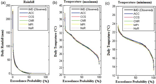
The exceedance probability curves of the observed and bias corrected GCM precipitation (1971–2005) and temperature (minimum and maximum) on the daily time scale are illustrated in Fig. 2. For precipitation, all the model results are clustered throughout (Fig. 2(a)), which might be because of all GCM outputs were from the same modelling centre (CORDEX). However, very close relation was noted between observed and GCM precipitation. For maximum (T_max) and minimum (T_min) temperatures (Fig. 2(b) and c)), all the model results are also close to the observed data. Op de Hipt et al. (2018) found approximately similar results after bias correction of precipitation for a tropical catchment in Burkina Faso, West Africa.

Figure 2. Exceedance probability curve for (a) rainfall, (b) maximum temperature (c) minimum temperature for the historical observed and five different GCMs.

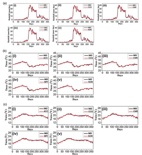
In addition, the long-term average daily data of the observed variables were compared with long-term average daily data of GCM-simulated variables from 1979 to 2005 at a daily timescale for an average of all grids within the VRB (Fig. 3). The GCMs could successfully represent the trend of the rainfall and temperature climatology (Fig. 3(a)) after bias correction. Hence, downscaled variables satisfactorily represent the climatic conditions of the study area and were further used in the SWAT model.

Figure 3. GCMs climatology (red) compared with observed climatology (black) for daily (a) rainfall, (b) maximum temperature and (c) minimum temperature from 1971 to 2005.

3.4 Determination of effects of land cover and climate changes on runoff and sediment yield

To distinguish the impacts of changes in land cover and climate on runoff and sediment yield, three scenarios were examined. The first two scenarios were rooted to one factor at a time approach (Li et al. 2009, Chawla and Mujumdar 2015, Zuo et al. 2016), where only one factor was changed at a time while leaving others constant. Therefore, climate was kept constant and land cover was changing in the first scenario and vice versa in the second one. The first and second scenarios revealed the respective influence of land cover and climate changes on the runoff and sediment yield with time. To identify the impacts of future climatology, GCM outputs for a future period were used in three time slices: T1 (2010–2040), T2 (2041–2070), and T3 (2071–2099). However, in the real case, land cover and climate change concurrently affect runoff and sediment yield, as described in the third scenario. In the third scenario, the SWAT model was run to obtain the baseline period (1985–2010) and projected for future period (2026–2035) with climate and 2030 land cover data. For quantifying the decadal changes in runoff and sediment yield, the baseline and future periods were divided into four periods: P1 (1986–1995), P2 (1996–2005), P3 (2006–2010), and P4 (2026–2035). The percentage contributions of land cover and climate to Q_int (integrated Runoff) and SY_int (integrated sediment yield) were computed as follows (Chawla and Mujumdar 2015):

(3) $\left\{\frac{\begin{array}{c}Min\left({\mathrm{\Delta }}_{\mathrm{i}\mathrm{j}}\right)\\ i=1,2,\dots p\\ j=1,2,\dots p\end{array}+\begin{array}{c}Max\left({\mathrm{\Delta }}_{\mathrm{i}\mathrm{j}}\right)\\ i=1,2,\dots p\\ j=1,2,\dots p\end{array}}{{\mathrm{\Delta }}_{\mathrm{i}\mathrm{j}}+\zeta \begin{array}{c}Max\left({\mathrm{\Delta }}_{\mathrm{i}\mathrm{j}}\right)\\ i=1,2,\dots p\\ j=1,2,\dots p\end{array}}\right\}$(3)

Notably, future land cover is also projected for assessment of impact of land cover change for the future time period in the VRB. In addition, the individual and combined impacts of land cover and climate on future runoff and sediment yield were assessed. The details of the methodology used are described in Fig. 4.

3.5 SUFI-2 calibration and sensitivity analysis

The SUFI-2 algorithm was applied for the optimization of hydrological parameters for runoff and sediment yield estimation. To identify the important parameters, the Latin Hypercube (LH) One Factor at a Time approach (Van Griensven et al. 2006) was used. It is a loop process and every loop begin with LH points. The partial effect S_ij for each parameter e_i around every LH point is estimated as follows (Abbaspour 2007).

(4) $\gamma \mathrm{j}=\frac{\left({\sum }_{\mathrm{i}=1}^{\mathrm{p}}{\sum }_{\mathrm{k}=1}^{\mathrm{r}}{\xi }_{\mathrm{i}\mathrm{j}\mathrm{k}}\right)}{\mathrm{p}\mathrm{r}}\mathrm{f}\mathrm{o}\mathrm{r}\mathrm{j}=1,2,\dots ,\mathrm{q}$(4)

where M (.....) denotes model function, f_i is the fraction by which e_i parameters varied, which is actually pre-set constant and specifies to LH sample points.

The final effect was the average of the fractional effects of the individual loop for entire LH points that are graded afterward in such a way that the rank of large effect was equivalent to the entire count of parameters. The detailed methodology of calibration is shown in Fig. 4.

Figure 4. Methodology and overview of the work.

The SUFI-2 algorithm provides information on model sensitive parameters by using the t-test, which estimates the relative importance of each parameter (provide measure of sensitivity). A larger t value indicated more sensitive parameters. While, p values determined the significance of the sensitivity and p value of nearly zero indicates higher sensitivity (Abbaspour et al. 2007). The overall model accuracy for hydrologic parameters was calculated by three statistical procedures which are the Nash-Sutcliffe coefficient (E_NS), coefficient of determination (R²) and percent bias (PBIAS) as given below:

(5) $Y=b0+b_1\left(\omega \right)+b_2\left(\nu \right)+b_3\left(H\right)+b_{12}\left(\omega \nu \right)+b_{13}\left(\omega H\right)+b_{23}\left(\nu H\right)+b_{11}\left(\omega 2\right)+b_{22}\left(\nu 2\right)+b_{33}\left(H2\right)$(5)

(6) $Y=3.9655-0.00345083\omega -0.0815667\nu -0.0187167H+1.42917E-06{\omega }^2+4.65185E-04{\nu }^2-9.833E-05H^2+2.9E-05\omega \nu +4.25E-06\omega H-3.5667E-05\nu H$(6)

(7) $\hat{\gamma }={\gamma }_m+\sum _{i=1}^0(\widehat{{\gamma }_i}-{\gamma }_m)$(7)

where n is the number of data records, O_i is the measured hydrologic parameters, O_avg is the average of measured data, S_i is the simulated data, and S_avg is the average of simulated data.

4 Results

4.1 Land cover change in the period 1972–2030

As discussed earlier, LCM model was developed for future land cover projection and calibration was carried out using available 2014 land cover map. The Idrisi model performance for land cover projection was acceptable (Fig. 5), with a small variation in agriculture (+2.40%), evergreen forest (–1.98%) and plantation (–0.80%). The deviation noted for plantation may have been due to the confusion of signature between plantation and mixed forest, which are very difficult to distinguish during the land use classification. The slight increase in medium dense urbanization may have occurred because the signatures of medium dense urbanization and barren area were similar during classification. In the classified images, water and grassland constituted 0.97% and 1.09% of the VRB, respectively, which was considered to remain constant throughout the model run. The overall resemblance between classified and modelled land cover images was 85%, which is in the reliable limit (Wu et al. 2009).

Figure 5. Land cover maps for 1972, 1979, 1988, 2000, 2014 (actual), 2014 (projected) and 2030 for VRB.

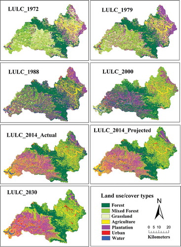
The temporal land cover maps from 1972 to 2030 are presented in Fig. 5 and land cover percentage in the VRB is listed in Table 3. Here, Sankey diagram (Cuba 2015) is used to understand the variation of land cover matrices with various time periods. The illustrated Sankey diagram in Fig. 6 visualizes land cover persistence and change occurring for five time periods (1972–1979, 1979–1988, 1988–2000, 2000–2014 and 2014–2030) in the VRB. The stacked bars represent the relative amount of each land cover type in 1972, 1979, 1988, 2000, 2014 and 2030. The height of each component in the stacked bars is proportional to the relative abundance of the represented land cover category in the study area. Forest (evergreen and mixed) is predominant in all time periods and contributing 55.1% in 1972, 58.5% in 1979, 63.9% in 1988, 62.3% in 2000, 57.1% in 2014 and 50.34% in 2030 of the total area (Fig. 6). The urban area and small amount of water bodies have increased, and grassland has decreased throughout the time periods. The agriculture area has slightly decreased in 1972–1979 and 1979–2000, but greatly increased in the periods 2000–2014 and 2014–2030. Finally, the spatial extent of plantation has increased in the periods 1972–1979, 1979–1988, but decreased in the period 1988–2000 and then increased in the periods 2000–2014 and 2014–2030.

Table 3. Land cover analysis of VRB for 1972, 1979, 1988, 2000, 2014 and 2030. EF: evergreen forest, MF: mixed forest, Ag: agriculture, GL: grassland, PT: plantation.

LC Type	Area (% of total area of 2517.2 km^2)
	1972	1979	1988	2000	2014	2030
Water	0.6	0.6	0.9	1.2	1.0	0.97
EF	24.2	26.1	39.6	37.5	29.0	25.23
MF	30.9	32.4	24.3	24.8	28.1	25.11
Ag	4.7	4.5	4.3	12.8	16.9	21.82
GL	28.2	16.7	5.5	4.6	1.1	0.96
PT	10.8	18.9	24.2	16.7	20.6	20.88
Urban	0.7	0.8	1.2	2.5	3.5	5.00

Figure 6. Sankey diagram for comparison of land cover dynamics in five time intervals defined by six land cover maps from the years 1972, 1979, 1988, 2000, 2014 and 2030.

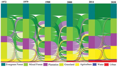
In Fig. 6, the vertically measured thickness of each horizontal line is proportional to the size of the land area that experiences the corresponding persistence or transition. The increase of evergreen forest area observed from 1972 to 1979 is noticed to be largely conversion of mixed forest and plantation (3.22% and 2.65%, respectively) and from 1979 to 1988 by mixed forest, plantation, and grassland (10.59%, 5.502% and 4.04%, respectively), but decrease from 1988 to 2030 is observed to mostly conversion into mixed forest, plantation, and grassland. The mixed forest category observed to increase from 1972 to 1979 by mainly conversion of grassland into mixed forest and decrease from 1979 to 1988 because of conversion into evergreen forest and plantation. The inter conversion of mixed forest is noticed after 1988–2030 but small amount of net change is found. Plantation increased from 1972 to 1988 due largely to conversion of mixed forest and grassland into plantation, but decreased in 2000 mostly because of conversion into forest (evergreen and mixed) and then expected to increase till 2030 by mostly conversion from evergreen forest. Grassland is decreased throughout the study period (1972–2030) and mostly conversion into mixed forest, plantation and agriculture. Agriculture area increases mostly because of transition of grassland, plantation, and mixed forest. Urban area is increased throughout the study period by conversion of mostly agriculture, grassland and slightly by other land cover categories.

The results indicate that the expansion of mostly agriculture and urbanization in the VRB will lead to less vegetation and loss of natural soil nutrients, which may affect runoff, sediment yield and soil productivity in the future. By contrast, an increase of 144.9 km² plantation areas from 1972 to 2030 indicates that previous loss of natural vegetation will lead the local people to reforestation to manage through the dearth of wood and fuel wood for different purposes. As demonstrated here, Sankey diagrams can potentially be used as a suitable replacement for the land cover matrices if the size of all components of the diagram were labelled (Cuba 2015). Such labels might not be able to be included in a static diagram due to limits on figure space.

4.2 Sensitivity analysis for surface runoff and sediment yield

The sensitive parameters for runoff and sediment yield were determined during calibration of the SWAT model with their statistics and ranking of sensitivity, as listed in Table 4. The most sensitive parameters for runoff were SCS-CN, followed by the deep aquifer percolation factor (RCHRG_DP), available water capacity of the soil layer (SOL_AWC), and other parameters (Table 4). The most sensitive parameters for sediment yield were the USLE support practice factor (USLE_P), followed by USLE soil erodibility factor (USLE_K), sediment concentration in lateral and groundwater flow (LAT_SED), and other parameters (Table 4). For the runoff, the parameters related to base flow and surface runoff has almost equally sensitive; by contrast, for sediment yield, the parameters related to the landscape were more sensitive than the sediment yield from the channel. Furthermore, for runoff, such as available water capacity (SOL_AWC) and surface runoff lag time (SURLAG), are further sensitive to sediment yield because the SWAT model is an inclusive model, which calculate process-based relations, such that numerous factors affect simultaneously. Here, sediment yield is influenced by surface runoff (Arnold et al. 2012).

Table 4. Streamflow and sediment yield parameters subjected to calibration and sensitivity analysis.

Process	Parameter (Discharge)		Global sensitivity			Process	Parameter (Sediment yield)		Global sensitivity
	Code	FV	p value	t value	Rank		Code	FV	p value	t value	Rank
Surface runoff	CN2	0.03 (r)	0.000	44.617	1	Sediment from landscape	SOL_AWC	0.202 (v)	0.000	12.387	1
	SOL_AWC	0.35 (v)	0.000	−26.148	3		USLE_P	0.026 (v)	0.000	−8.564	2
	ESCO	0.13 (v)	0.200	−1.280	8		USLE_K	0.483 (v)	0.000	−5.859	3
	EPCO	0.68 (v)	0.623	−0.491	9		LAT_SED	78.34 (v)	0.190	−1.309	7
	SUR_LAG	4.69 (v)	0.003	−2.908	6		HRU_SLP	0.005 (r)	0.442	−0.768	8
Base flow	ALPHA_BF	0.19 (v)	0.859	0.177	10	Sediment from channel	SLSUBBSN	0.005 (r)	0.836	0.205	9
	GW_DELAY	35.5 (v)	0.000	−11.561	4		SURLAG	0.022 (v)	0.166	−1.384	6
	GW_REVAP	0.16 (v)	0.001	−3.158	5		SPCON	0.0013 (v)	0.874	0.157	10
	RCHRG_DP	0.08 (v)	0.000	−31.843	2		CH_ERODMO	0.414 (v)	0.050	1.958	5
	GWQMN	12.05 (v)	0.007	−2.669	7		CH_N2	0.133 (v)	0.014	2.450	4

FV: fitted value, (r) is the existing value that is multiplied; (v) is the existing value that is replaced by the given value.

4.3 Model calibration and validation

The SWAT model was calibrated at gauging station in sub-basin 26 for runoff and sediment yield by using 2000 land cover data. The comparisons between simulated and observed on monthly basis during the period of calibration (1 January 1991 − 31 December 2000) and validation (1 January 2001 − 31 December 2010) for runoff and sediment yield are presented in Figs. 7 and 8, respectively. The sensitive parameters and fitted values used for calibration of runoff and sediment yield are listed in Table 4. The E_NS, R² and PBIAS values for monthly calibration and validation are presented in Table 5. The R² and E_NS values for runoff were greater than 0.85, and the PBIAS values were ±20% for both calibration and validation time periods. The R² and E_NS values for sediment yield are higher than 0.65, whereas the PBIAS values were in the range of ±10%, suggesting favourable model performance (Moriasi et al. 2007).

Table 5. Model performance criteria for calibration and validation.

Items	Land cover 2000
	Calibration (1991–2000)		Validation (2001−2010)
Streamflow Sediment yield Streamflow Sediment yield
NS	0.88	0.79	0.84	0.76
R^2	0.94	0.84	0.93	0.73
PBIAS	10.42	4.35	16.72	12.26

Figure 7. Comparison between the observed and simulated monthly streamflow for the (a) calibration and (b) validation and scatterplot between the observed and simulated streamflow for the (c) calibration and (d) validation.

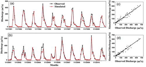
Figure 8. Comparison between the observed and simulated monthly sediment yield for the (a) calibration and (b) validation and scatterplot between the observed and simulated sediment yield for the (c) and calibration (d) validation.

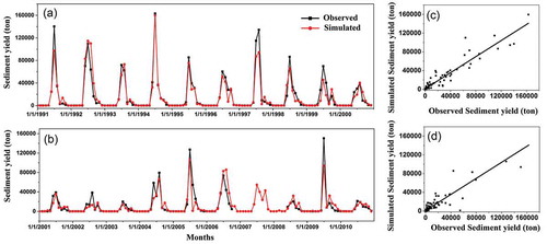
The overall consistency of the model was acceptable, as shown in Table 5. The trends of simulated and observed data were identical during most of the years (Figs. 7 and 8). However, the streamflow and sediment yield were slightly underestimated for the extreme monsoon months (July and August). In other words, peak streamflow and sediment yield events were not adequately represented by the corresponding observed data. This is because of the impediments of the SCS-CN technique and presence of small dam for irrigation in the upstream. In the SWAT model, the SCS-CN technique does not consider the rainfall intensity and duration, but mean daily precipitation as an input (Nie et al. 2011). In the VRB, precipitation events often persist short duration with high intensity. In practice, more sediment was produced by short-duration rainfall with high-intensity than was specified by the model based on daily mean precipitation (Xu et al. 2009). On the other hand, the presence of dam (for irrigation) can reduce sediment yield. In general, the reliability between the simulated outputs by the model and the observed values as well as their R², E_NS, and PBIAS values showed that the model performed well for a monthly time scale.

4.4 Impacts of land cover change on runoff and sediment yield at the basin scale

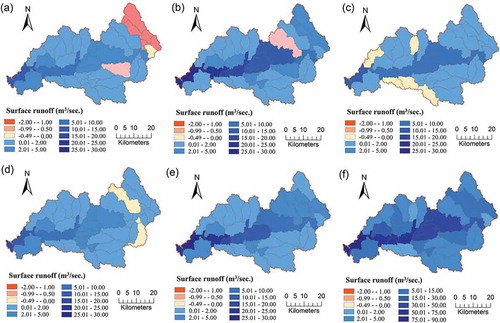
In VRB, vital changes are reported in the land cover types of forest, grassland, plantation, agriculture, and urban areas. The spatial distribution of impacts of change in land cover on runoff is estimated using the climate data during 1981−2010 and presented in Fig. 9. The continuous increase in overall runoff (including all sub-basins) from 1972 to 1979 was 1.14%, for 1979–1988 it was 2.29%, for 1988–2000 it was 0.85% and for 2000–2014 it was 1.25%; the plausible increment from 2014 to 2030 will be 1.89%. In addition, the maximum change in runoff was noted at the sub-basins near the channel (21, 25, 26, 27, 32, 34, etc.) as shown in Fig. 9, which may have contributed increased direct runoff (Fig. 9(b)). Compared with the present land cover (2014), the average runoff will be increased by 24.60 m³/s (1.89%) until 2030, however, the average annual runoff will increase by 0.08%, with a 7.66% overall increase from the baseline land cover (1972) to projected land cover (2030) in the VRB.

Figure 9. Spatial distribution of change in the surface runoff for land cover map between 1972 and 2030: (a) 1972–1979; (b) 1979–1988; (c) 1988–2000; (d) 2000–2014; (e) 2014–2030; and (f) 1972–2030.

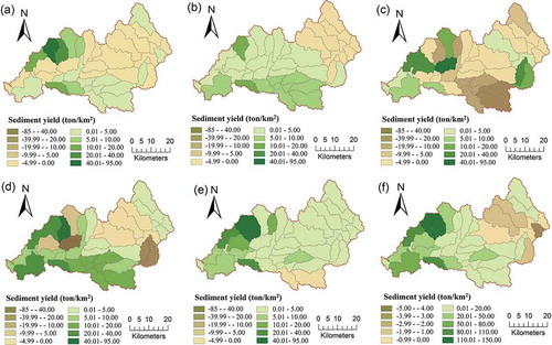
The spatial distribution of sediment yield is presented in Fig. 10. The results revealed a continuous increase in overall sediment yield of 0.076% from 1972 to 1979, 16.25% from 1979 to 1988, 6.07% from 1988 to 2000, and 14.13% from 2000 to 2014 and a plausible increment of 13.01% from 2014 to 2030. Furthermore, compared with the present land cover (2014), the average sediment yield will be increased by 29.83 ton/km² (13.01%) until 2030. However, the average annual sediment yield will be increased by 1.62 ton/km²/year, with overall increase of 95.97 ton/km² from the baseline land cover (1972) to projected land cover (2030) in the VRB.

Figure 10. Spatial distribution of change in the sediment yield for land cover map between 1972 and 2030: (a) 1972–1979; (b) 1979–1988; (c) 1988–2000; (d) 2000–2014; (e) 2014–2030; and (f) 1972–2030.

4.5 Impacts of climate change on runoff and sediment yield at basin scale

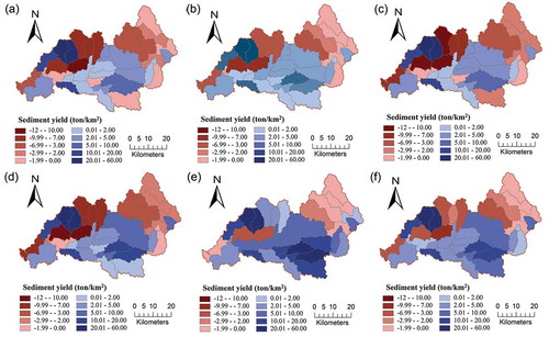
To compute the change in runoff and sediment yield, the SWAT model was run using five downscaled, bias-corrected GCMs outputs for RCP4.5 and RCP8.5 and the simulated results were compared with those of the baseline period (1981–2010). The obtained simulation results are referred to as Q_clim and SY_clim hereafter. The simulated Q_clim and SY_clim for the future period under RCP4.5 and RCP8.5 scenarios are compared to the corresponding values of all sub-basins from the baseline period. The change in annual Q_clim and SY_clim for all the time slices was moderate to considerable for the forthcoming time periods under RCP4.5 and RCP8.5 climate change scenarios (Figs. 11 and 12). In general, Q_clim is predicted to decrease in most sub-basins, mainly near the main channel and also in very few sub-basins (Fig. 11). In particular, the Q_clim decreased from the baseline period by 10.93%, 5.21% and 6.33% under RCP 4.5 and 9.89%, 5.11%, and 5.67% for RCP8.5 during T1, T2 and T3, respectively. SY_clim was predicted to decrease by 23%–31% under RCP4.5 and by 5.7–26% under RCP8.5 in all future climate time slices (T1, T2 and T3) compared with baseline period. Notably, the variation in the percentage in different climatic periods will largely be due to variation in precipitation in the corresponding period in the VRB in the future. The results of spatial distribution of RCP4.5 and RCP8.5 (Fig. 11) clearly indicated that only few sub-basins, such as 3, 12, 17, 18, 19, 24, 28 and 35, had increased Q_clim, whereas the Q_clim of all other sub-basins notably decreased from 3.1 to 109.4 m³/s in T1, 2.7 to 47.34 m³/s in T2, and 1.4 to 43.3 m³/s in T3 under RCP4.5; similar results were noted for RCP8.5, except for that in T2. Figure 12 shows the spatial distribution of SY_clim and observed that in few sub-basins, these is major increase in sediment yield for both RCP scenarios and all time slices.

Figure 11. Spatial distribution of change in the future surface runoff for three different scenarios of climate change between 2011 and 2099 for RCP4.5 and RCP8.5: (a) RCP4.5 (2011–2040); (b) RCP4.5 (2041–2070); (c) RCP4.5 (2071–2099); (d) RCP8.5 (2011–2040); (e) RCP8.5 (2041–2070); and (f) RCP8.5 (2071–2099).

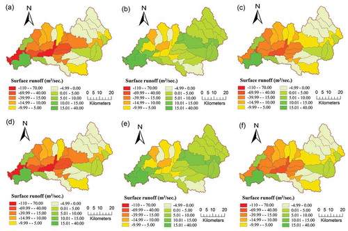
Figure 12. Spatial distribution of change in the future sediment yield for three different scenarios of climate change between 2011 and 2099 for RCP4.5 and RCP8.5: (a) RCP4.5 (2011–2040); (b) RCP4.5 (2041–2070); (c) RCP4.5 (2071–2099); (d) RCP8.5 (2011–2040); (e) RCP8.5 (2041–2070); and (f) RCP8.5 (2071–2099).

4.6 Combined impacts of land cover and climate change on runoff and sediment yield at basin scale

The assessment of the impacts of land cover changes primarily required Q_int and Q_clim for runoff as well as SY_int and SY_clim for sediment yield for the same period. The values of Q_int and Q_clim, as well as SY_int and SY_clim, were compared on the basis of corresponding simulations acquired in the same settings of the hydrological model and climatic conditions. This technique enables the only change among the two scenarios to the land cover inputs into the hydrological model (Chawla and Mujumdar 2015). Thus, the subtraction of the two scenarios, Q_int − Q_clim, and SY_int − SY_clim is considered the exclusive contribution of land cover of runoff and sediment yield (hereafter Q_lc and SY_lc, respectively). To separate the role of land cover and climate changes from Q_int and SY_int, linear responses of land cover and climate change to the runoff and sediment yield are considered. Further, annual average ETpot and ETact for different time periods are presented in Table 6.

Table 6. Contribution of land cover and climate to the streamflow and sediment yield for different time periods. P: precipitation; ETpot: potential evapotranspiration, ETact: actual evapotranspiration.

	P1	P2	P3	P4 (RCP 4.5)	P4 (RCP 8.5)
	1986–1995	1996–2005	2006–2010	2026–2035	2026–2035
P (mm/year)	2091.2	1849.1	2107.7	1913.3	1864.3
ETpot (mm/year)	1359.1	1186.13	1348.5	1205.4	1162.6
ETact (mm/year)	880.6	774.7	855.8	751.9	734.4
Streamflow
Qint (mm/year)	836.32	741.23	845.63	724.32	709.21
Qclim (mm/year)	812.67	712.54	776.21	639.13	625.23
Qclim (%)	97.21	96.16	91.86	88.24	88.16
Qlc (mm/year)	23.65	28.69	69.42	85.19	83.98
Qlc (%)	2.79	3.84	8.14	11.76	11.84
Sediment yield
SYint (10^5 t/year)	7.41	5.64	8.05	5.46	5.71
SYclim (10^5 t/year)	7.01	4.71	6.52	3.85	4.00
SYclim (%)	94.60	84.10	80.99	70.51	70.05
SYlc (10^5 t/year)	0.40	0.93	1.53	1.61	1.71
SYlc (%)	5.40	15.90	19.01	29.49	29.95

In this case study, Q_int, Q_clim, SY_int and SY_clim were obtained from the four periods P1, P2, P3, and P4. However, P4 comprised RCP4.5 and RCP8.5 scenarios for the future projection of the impacts of land cover and climate changes. Then, Q_int and Q_clim were used for estimating Q_lc, whereas SY_int and SY_clim for estimating SY_lc. Table 6 lists the results of the combined effects of land cover and climate changes. When Q_lc (%) and SY_lc (%) were assessed across the different periods, the gradual increases were noted in the contribution of runoff and sediment yield (Table 6). The proposed methodology for separating the hydrological impacts of land cover and climate changes were also applied for future land cover (2030) and climate (2025–2035) for understanding the future plausible impacts. The results for P4 (RCP4.5) and (RCP8.5) are presented in Table 6 after using 2030 land cover for assessing runoff and sediment yield. In P4, the contribution of changes in land cover to runoff and sediment yield will be increased compared with P3. Results also suggest that climate is more dominant than land cover on runoff and sediment yield (Table 6).

5 Discussion

The mean annual water balance can be represented by the difference between average annual precipitation and runoff, ET and change in the different water storage capacity of a concerned river basin (Yan et al. 2013). The various types of LULC effects on the hydrology in a basin can balance each other, and net observed change can sometimes be relatively small at the basin scale. In the present case also, some water (except runoff and ET) goes to deep groundwater recharge and other purposes such as irrigation or other activities that are not considered in the SWAT model. Therefore, long-term discrepancy in the water budget at the basin scale may be the result. Further, details of the limitations and uncertainty of the study and of the SWAT model are discussed in Section 5.1.

The change in land cover has a great effect on historical and near future runoff and sediment yield in the study area. The maximum change in runoff occurred from 1979 to 1988 which could be due to deforestation (mixed forest) and conversion of grassland areas into plantation areas. Furthermore, urban expansion may have contributed to increase in runoff. Minimum change in runoff was found in the period 1988–2000, potentially because of small amount of deforestation (<2% evergreen forest). However, there is increase in surface runoff mainly because of agriculture (8.5%) and urban expansion (1.3%). During the same time, areas of plantation (such as rubber plantation) were converted into agricultural areas (Table 3), potentially increasing runoff. Compared with the present (i.e. 2014), the runoff may increase by 1.89% by 2030, mainly because of deforestation (3.7%) and the expansion of agricultural (4.92%) and urban (1.5%) areas in the period (2014–2030). The overall analysis at the sub-basin level indicates that the increase in runoff occurs in all parts of the basin, but more in the central part (along a river channel) (Fig. 9(f)). This is because of the expansion of agricultural and urban areas along the river basin. Increased urbanization is generally associated with an increase in high flows and a decrease in low flows, because it increases impervious surface coverage and that, in turn, decreases the infiltration of rainfall and increases runoff (Yan et al. 2013, Sinha and Eldho 2018). Urban areas usually result in a decrease in ET, percolation and groundwater flow and an increase in surface runoff. Similar conclusions were drawn by many studies (e.g. Nie et al. 2011, Wang et al. 2011). The maximum change in sediment yield occurred in the period 1979–1988 (2.29%), similar to the results of runoff (i.e., increase in runoff can increase sediment yield). This could have occurred because of deforestation (mixed forest) and conversion of grassland into unorganized plantation, leading to reduced soil compactness. Moreover, urban expansion may have contributed to increased sediment yield. The overall sediment yield increased mainly downstream of the river basin and slightly decreased from upstream (particularly sub-basins 3, 4, 10, 15 and 24). By contrast, the dynamic change in sediment yield in different time period may indicate that change in land cover from one type to other can manage sediment yield itself in the river basin. Forest and grassland can reduce the sediment yield, but agricultural and urban areas can generate more sediment yield in the basin (Khoi and Suetsugi 2014). However, it is reported that due to less pressure on using forest goods, the total forest cover in India has increased in the period 2005–2013 by 0.63% (http://www.niti.gov.in) and may continue to increase in the future too. This might have substantial effects on the hydrology, reducing the soil erosion and improving the overall hydrological conditions.

The results of climate change impact study indicate that Q_clim and SY_clim decreased overall under both RCP scenarios and in all three time slices in comparison to the baseline period and emphasize the need for water resource management. The results clearly indicate most of the central part of the basin and along the river channel has decreasing runoff, while the upstream and some of the downstream sub-basins (mainly 19 and 35) show increasing runoff (Fig. 11). Furthermore, the runoff and sediment yield did not always follow the same trend in response to climate change. For instance, in the period 2041–2070 under RCP4.5 and RCP8.5 scenarios, annual runoff and sediment yield appeared to decrease, potentially because of decreased annual rainfall and increased air temperature. However, in the period 2071–2099, a slight increase (<1.5%) of annual runoff and sediment yield is observed in comparison to the period 2041–2070, with an increase in precipitation by 51 mm. Hence, the main driving forces of runoff and sediment yield in the VRB are precipitation and temperature. Overall, the decreasing precipitation and increasing temperature may have reduced water availability, ultimately reducing vegetation growth and thus exacerbating water scarcity and soil erosion. The climate in the study area is characterized by the southwest monsoon, which is significantly declining in India (Krishnakumar et al. 2009). Soman et al. (1988) reported that annual precipitation showed a significant decreasing trend over Kerala where the VRB is located. They reported changes in characteristics, such as a decrease in water vapour and summer monsoon circulation, which affect the onset of the monsoon that is usually around 1 June ±7 days and is likely to shift further (https://shodhganga.inflibnet.ac.in). Therefore, farmers may have to sow seeds for their crops much later than they do now and there is a chance that there will be a reduction in productivity of some crops. In Kerala, paddy productivity is likely to decline due to long-term climate change, with increases in temperature followed by unusual summer rains (https://shodhganga.inflibnet.ac.in). The results of this study show decreased annual Q_clim and SY_clim patterns under RCP4.5 and RCP8.5 scenarios in all three time slices; precipitation in the VRB is shown to potentially decline in the future period in comparison to the baseline period. In addition, Q_clim and SY_clim in the region are strongly related to ecosystem physical conditions. Therefore, it is essential to better understand the impacts of climate change on streamflow and sediment yield for sustenance of agricultural production and sustainable water resource management in the future.

The comparison between land cover and climate change impacts on runoff and sediment yield reveal that the climate change is more dominant than the land cover change (Table 6). Similar results have been reported for runoff in Hoeya River basin, South Korea (Kim et al. 2013) and the Upper Ganges Basin (Chawla and Mujumdar 2015). However, the effects of land cover (Q_lc) are projected to increase from 2.79% to 29.95% in the future (Table 6). Notably, runoff and sediment yield are shown to be highly sensitive to agriculture and urbanization but the spatial extent of urbanization in the whole study area was much lower than the total area (5%), which may be the reason for the smaller influence of land cover change to runoff and sediment yield. However, the scenario under both land cover and climate changes showed larger impacts. In addition, the contribution of land cover changes in P4 to runoff and sediment yield will be increased compared to P3. This could be due to an increase in urban and agricultural areas and decrease in forest area from P3 to P4. Furthermore, the influence of LULC to runoff and sediment yield will be slightly (but negligibly) higher for RCP4.5 than for RCP8.5 (Table 6) because of the stronger climate change signal in the latter scenario. The impervious urban surface coverage hampered infiltration rate of rainfall, leading to increased surface runoff, potentially increasing sediment load; the increase of surface runoff can enhance the impacts of climate change. Hence a revised plan of water resource management considering future land cover and climate change for runoff and sediment yield is required in the basin.

5.1 Limitations and uncertainty

The SWAT model is an effective and useful tool for assessment of LULC and climate change impacts on runoff and sediment yield, but some limitations and uncertainty exist in the model. The runoff and sediment yield in the basin may be influenced by the resolution of the DEM, soil parameters, LULC and HRU delineation (Gassman et al. 2007). In the climatic parameters, precipitation (Keesstra et al. 2019) and temperature are the main factors which affect the runoff and sediment yield. Therefore, it is important to have good quality (bias corrected) data for the simulation of the hydrological processes to reduce the uncertainty in the results. Furthermore, several empirical and quasi-physical equations in the SWAT model, such as the SCS-CN method and MUSLE method (Neitsch et al. (2011)), were developed based on climatic conditions in the USA, which may not be appropriate for India. The SCS-CN method does not reflect event-based flow assessment and the MUSLE method does not include the processes occurring in the river basin, such as landslides which may cause soil erosion. This may lead to some uncertainty in the results for runoff and sediment yield simulation, mainly at the daily time scale. Additionally, calibrated parameters are conditioned on the choice of objective function, the types and length of measured data, and the procedure used for calibration (Yang et al. 2008). Despite these limitations and uncertainties, the simulation results for monthly runoff and sediment yield in the present study are satisfactory according to norms given by Moriasi et al. (2007).

The proposed approach can be applied to other large river basins by using a thoroughly calibrated and validated hydrological model. We used only Landsat data for land cover in this study, but further research may focus on different sources of land cover data such as MODIS, Global Land Cover Characterization (GLCC) or Terrapop, for the assessment of uncertainty related to land cover. Furthermore, in this study, only one hydrological model (SWAT) was used, but the application of a multi-model (variable infiltration capacity model, SHETRAN etc.) technique might improve the understanding of the uncertainty regarding the model outputs. In addition, quantile-based bias correction for climate variables is used but further different techniques of bias correction such as linear scaling or local intensity (LOCI) scaling might be more efficient for the analysis of hydrological parameters. Additional optimization techniques, such as GLUE, Parasol and Monte Carlo, can help in understanding the parameter uncertainty in the river basin.

6 Conclusions

In this paper, a methodological framework for study of the impacts of historical and future land cover and climate change on runoff and sediment yields in river basin is developed and demonstrated for the Valapattanam River Basin (VRB) in South India. The SWAT model is used as the hydrological model and LCM is used for land cover projection. In the VRB, forest (evergreen and mixed) and grassland were the most predominant land cover types in 1972 and these were projected to decrease by 4.76% and 27.24%, respectively, by 2030. The Sankey diagram is used represent the land cover variation. The land cover change assessment indicated that forest areas were mainly converted to plantation or grassland areas, followed by agricultural and urban areas. The runoff and sediment yield are highly sensitive to the expansion of agricultural and urban areas. The analysis to identify the separate impacts of changes in land cover and climate, as well as their combined effects, reveals that the contribution of climate to the runoff and sediment yield is very high (>85%). Furthermore, the future land cover change will have a more important role than the historical land cover change did. In addition, future rainfall change is projected to decrease the runoff and sediment yield under both RCP4.5 and RCP8.5 emissions scenarios. The combined impacts of future changes in land cover and climate on runoff and sediment yield are similar to those of climate change alone.

Understanding the combined and individual impacts of future land cover and climate changes on runoff and sediment yield is essential for sustainable water resource planning and management in a river basin. For the case study of the VRB, annual runoff and sediment yield are likely to become highly affected in the future. The long-term planning for water resources in the river basin must be adjustable and resilient to the changing pattern of these impacts. The methodological framework used in this study can be extended to other river basins for appropriate water resources management.

Acknowledgements

The authors acknowledge the Department of Science and Technology for financial support to this study. We wish to express our deep gratitude to Central Water Commission and Indian Meteorological Department India for providing hydrological and meteorological data. Authors also acknowledge the sponsorship of the project entitled “Impacts of Climate Change on Water Resource in River Basin from Tadri to Kanyakumari” by INCCC, Ministry of Water Resource, Gov. of India.

Disclosure statement

No potential conflict of interest was reported by the authors.

Additional information

Funding

This work was supported by the Indian Institute of Technology Bombay [Research Scholar].

Notes

¹ http://censusindia.gov.in/

² https://www.indiastat.com/

References

- Abbaspour, K.C., 2007. User manual for SWAT-CUP, SWAT calibration and uncertainty analysis programs. Eawag, Duebendorf, Switzerland: Swiss Federal Institute of Aquatic Science and Technology.
- Abbaspour, K.C., et al., 2009. Assessing the impact of climate change on water resources in Iran. Water Resources Research, 45 (10). doi:10.1029/2008WR007615
- Abbaspour, K.C., et al., 2007. Modelling hydrology and water quality in the pre-alpine/alpine Thur watershed using SWAT. Journal of Hydrology, 333 (2–4), 413–430. doi:10.1016/j.jhydrol.2006.09.014
- Arnold, J.G., et al., 2012. SWAT: model use, calibration, and validation. Transactions of the ASABE, 55 (4), 1491–1508. doi:10.13031/2013.42256
- Arnold, J.G., et al., 1998. Large area hydrologic modeling and assessment part I: model development. JAWRA Journal of the American Water Resources Association, 34 (1), 73–89. doi:10.1111/j.1752-1688.1998.tb05961.x
- Azari, M., et al., 2016. Climate change impacts on streamflow and sediment yield in the North of Iran. Hydrological Sciences Journal, 61 (1), 123–133. doi:10.1080/02626667.2014.967695
- Barredo, J.I., et al., 2003. Modelling dynamic spatial processes: simulation of urban future scenarios through cellular automata. Landscape and Urban Planning, 64 (3), 145–160. doi:10.1016/S0169-2046(02)00218-9
- Bekele, E.G. and Knapp, H.V., 2010. Watershed modeling to assessing impacts of potential climate change on water supply availability. Water Resources Management, 24 (13), 3299–3320. doi:10.1007/s11269-010-9607-y
- Bussi, G., et al., 2016. Modelling the future impacts of climate and land-use change on suspended sediment transport in the River Thames (UK). Journal of Hydrology, 542, 357–372. doi:10.1016/j.jhydrol.2016.09.010
- CEPF, 2007. Ecosystem profile for the Western Ghats. Available from: https://ind01.safelinks.protection.outlook.com/?url=https%3A%2F%2Fwww.cepf.net%2Fsites%2Fdefault%2Ffiles%2Fwestern-ghats-ecosystem-profile-english.pdf&data=02%7C01%7Csathyan.dhanasekaran%40integra.co.in%7C4674c1fd9e474fd2acdf08d827a336c4%7C70e2bc386b4b43a19821a49c0a744f3d%7C0%7C1%7C637302929247191237&sdata=7u0VKF%2FqeusyVjrzxSanI%2F7VRVLAfRwVnlsnCxwInn0%3D&reserved=0 [accessed 14 Apr 2020].
- Chawla, I. and Mujumdar, P.P., 2015. Isolating the impacts of land use and climate change on streamflow. Hydrology and Earth System Sciences, 19 (8), 3633–3651. doi:10.5194/hess-19-3633-2015
- Cuba, N., 2015. Research note: sankey diagrams for visualizing land cover dynamics. Landscape and Urban Planning, 139, 163–167. doi:10.1016/j.landurbplan.2015.03.010
- Farjad, B., et al., 2017. An integrated modelling system to predict hydrological processes under climate and land-use/cover change scenarios. Water, 9 (10), 767. doi:10.3390/w9100767
- Fukhrudin, K.M., et al., 2013. Modeling the impact of land use changes on runoff and sediment yield in the Le Sueur watershed, Minnesota using GeoWEPP. Catena, 107, 35–45. doi:10.1016/j.catena.2013.03.004
- Garg, K.K., et al., 2013. Up‐scaling potential impacts on water flows from agricultural water interventions: opportunities and trade‐offs in the Osman Sagar catchment, Musi sub‐basin, India. Hydrological Processes, 27 (26), 3905–3921. doi:10.1002/hyp.9516
- Gassman, P.W., et al., 2007. The soil and water assessment tool: historical development, applications, and future research directions. Transactions of the ASABE, 50, 1211–1240. doi:10.13031/2013.23637
- Gebremicael, T.G., et al., 2013. Trend analysis of runoff and sediment fluxes in the Upper Blue Nile basin: A combined analysis of statistical tests, physically-based models and landuse maps. Journal of Hydrology, 482, 57–68. doi:10.1016/j.jhydrol.2012.12.023
- IPCC, 2013. The physical science basis. In: T.F. Stocker et al., eds. Contribution of working group I to the fifth assessment report of the intergovernmental panel on climate change. Cambridge, UK and York, NY, USA: Cambridge University Press, 1535 doi: 10.1017/CBO9781107415324
- Islam, S., Bari, M., and Anwar, F., 2014. Hydrologic impact of climate change on Murray–Hotham catchment of Western Australia: a projection of rainfall–runoff for future water resources planning. Hydrology and Earth System Sciences, 18 (9), 3591–3614. doi:10.5194/hess-18-3591-2014
- Jensen, J.R., 2005. Introductory digital image processing: a remote sensing perspective. 3rd ed. NJ: Upper Saddle River.
- Jiongxin, X., 2003. Sediment flux to the sea as influenced by changing human activities and precipitation: example of the Yellow River, China. Environmental Management, 31 (3), 0328–0341. doi:10.1007/s00267-002-2828-y
- Jordan, Y.C., Ghulam, A., and Hartling, S., 2014. Traits of surface water pollution under climate and land use changes: A remote sensing and hydrological modeling approach. Earth-Science Reviews, 128, 181–195. doi:10.1016/j.earscirev.2013.11.005
- Keesstra, S.D., et al., 2019. Coupling hysteresis analysiswith sediment and hydrological connectivity in three agricultural catchments in Navarre, Spain. Journal of Soils and Sediments, 19, 1598–1612. doi:10.1007/s11368-018-02223-0
- Khoi, D.N. and Suetsugi, T., 2014. Impact of climate and land-use changes on hydrological processes and sediment yield—a case study of the Be River catchment, Vietnam. Hydrological Sciences Journal, 59 (5), 1095–1108. doi:10.1080/02626667.2013.819433
- Kim, J., et al., 2013. Impacts of changes in climate and land use/land cover under IPCC RCP scenarios on streamflow in the Hoeya River Basin, Korea. Science of the Total Environment, 452, 181–195. doi:10.1016/j.scitotenv.2013.02.005
- Krishnakumar, K.N., Rao, G.P., and Gopakumar, C.S., 2009. Rainfall trends in twentieth century over Kerala, India. Atmospheric Environment, 43 (11), 1940–1944. doi:10.1016/j.atmosenv.2008.12.053
- Lenhart, T., et al., 2005. Considering spatial distribution and deposition of sediment in lumped and semi‐distributed models. Hydrological Processes, 19 (3), 785–794. doi:10.1002/hyp.5616
- Li, H., Sheffield, J., and Wood, E.F., 2010. Bias correction of monthly precipitation and temperature fields from Intergovernmental panel on climate change AR4 models using equidistant quantile matching. Journal of Geophysical Research: Atmospheres, 115, D10.
- Li, X. and Yeh, A.G.O., 2000. Modelling sustainable urban development by the integration of constrained cellular automata and GIS. International Journal of Geographical Information Science, 14 (2), 131–152. doi:10.1080/136588100240886
- Li, Z., et al., 2009. Impacts of land use change and climate variability on hydrology in an agricultural catchment on the Loess Plateau of China. Journal of Hydrology, 377 (1–2), 35–42. doi:10.1016/j.jhydrol.2009.08.007
- Lørup, J.K., Refsgaard, J.C., and Mazvimavi, D., 1998. Assessing the effect of land use change on catchment runoff by combined use of statistical tests and hydrological modelling: case studies from Zimbabwe. Journal of Hydrology, 205 (3–4), 147–163. doi:10.1016/S0168-1176(97)00311-9
- Lu, D. and Weng, Q., 2007. A survey of image classification methods and techniques for improving classification performance. International Journal of Remote Sensing, 28 (5), 823–870. doi:10.1080/01431160600746456
- Mango, L.M., et al., 2011. Land use and climate change impacts on the hydrology of the upper Mara River Basin, Kenya: results of a modeling study to support better resource management. Hydrology and Earth System Sciences, 15 (7), 2245. doi:10.5194/hess-15-2245-2011
- Mishra, A., Kar, S., and Singh, V.P., 2007. Prioritizing structural management by quantifying the effect of land use and land cover on watershed runoff and sediment yield. Water Resources Management, 21 (11), 1899–1913. doi:10.1007/s11269-006-9136-x
- Moriasi, D.N., et al., 2007. Model evaluation guidelines for systematic quantification of accuracy in watershed simulations. Transactions of the ASABE, 50 (3), 885–900. doi:10.13031/2013.23153
- Myers, N., et al., 2000. Biodiversity hotspots for conservation priorities. Nature, 403 (6772), 853. doi:10.1038/35002501
- Ndomba, P., Mtalo, F., and Killingtveit, A., 2008. SWAT model application in a data scarce tropical complex catchment in Tanzania. Physics and Chemistry of the Earth, Parts A/B/C, 33 (8–13), 626–632. doi:10.1016/j.pce.2008.06.013
- Neitsch, S.L., et al., 2011. Soil and water assessment tool theoretical documentation version 2009. Texas: Texas Water Resources Institute, Texas A&M University, College Station.
- Nie, W., et al., 2011. Assessing impacts of landuse and landcover changes on hydrology for the upper San Pedro watershed. Journal of Hydrology, 407 (1–4), 105–114. doi:10.1016/j.jhydrol.2011.07.012
- Op de Hipt, F., et al., 2018. Modeling the impact of climate change on water resources and soil erosion in a tropical catchment in Burkina Faso, West Africa. Catena, 163, 63–77. doi:10.1016/j.catena.2017.11.023
- Op de Hipt, F.O., et al., 2019. Modeling the effect of land use and climate change on water resources and soil erosion in a tropical West African catch-ment (Dano, Burkina Faso) using SHETRAN. Science of the Total Environment, 653, 431–445. doi:10.1016/j.scitotenv.2018.10.351
- Petit, C., Scudder, T., and Lambin, E., 2001. Quantifying processes of land-cover change by remote sensing: resettlement and rapid land-cover changes in south-eastern Zambia. International Journal of Remote Sensing, 22 (17), 3435–3456. doi:10.1080/01431160010006881
- Prowse, T.D., et al., 2006. Climate change, flow regulation and land-use effects on the hydrology of the Peace-Athabasca-Slave system; Findings from the Northern Rivers ecosystem initiative. Environmental Monitoring and Assessment, 113 (1–3), 167–197. doi:10.1007/s10661-005-9080-x
- Rientjes, T.H.M., et al., 2011. Changes in land cover, rainfall and stream flow in Upper Gilgel Abbay catchment, Blue Nile basin-Ethiopia. Hydrology and Earth System Sciences, 15 (6), 1979. doi:10.5194/hess-15-1979-2011
- Rounsevell, M.D.A., et al., 2006. A coherent set of future land use change scenarios for Europe. Agriculture, Ecosystems & Environment, 114 (1), 57–68. doi:10.1016/j.agee.2005.11.027
- Salvi, K. and Ghosh, S., 2013. High‐resolution multisite daily rainfall projections in India with statistical downscaling for climate change impacts assessment. Journal of Geophysical Research: Atmospheres, 118 (9), 3557–3578.
- Sinha, R.K. and Eldho, T.I., 2018. Effects of historical and projected land use/cover change on runoff and sediment yield in the Netravati river basin, Western Ghats, India. Environmental Earth Sciences, 77 (3), 111. doi:10.1007/s12665-018-7317-6
- Soman, M.K., Krishna, K.K., and Singh, N., 1988. Decreasing trend in the rainfall of Kerala. Current Science, 57, 7–12.
- Syvitski, J.P., et al., 2005. Predicting the flux of sediment to the coastal zone: application to the Lanyang watershed, Northern Taiwan. Journal of Coastal Research, 580–587. doi:10.2112/04-702A.1
- Tomer, M.D. and Schilling, K.E., 2009. A simple approach to distinguish land-use and climate-change effects on watershed hydrology. Journal of Hydrology, 376 (1–2), 24–33. doi:10.1016/j.jhydrol.2009.07.029
- USDA-SCS (United States Department of Agriculture – Soil Conservation Service), 1972. National engineering handbook, Section 4 hydrology. Chapter 4–10. Washington, USA: USDA-SCS.
- Van Griensven, A., et al., 2006. A global sensitivity analysis tool for the parameters of multi-variable catchment models. Journal of Hydrology, 324 (1–4), 10–23. doi:10.1016/j.jhydrol.2005.09.008
- Wada, Y., Van Beek, L.P.H., and Bierkens, M.F., 2011. Modelling global water stress of the recent past: on the relative importance of trends in water demand and climate variability. Hydrology and Earth System Sciences, 15 (12), 3785–3805. doi:10.5194/hess-15-3785-2011
- Wagner, P.D., et al., 2016. Dynamic integration of land use changes in a hydrologic assessment of a rapidly developing Indian catchment. Science of the Total Environment, 539, 153–164. doi:10.1016/j.scitotenv.2015.08.148
- Wagner, P.D., Kumar, S., and Schneider, K., 2013. An assessment of land use change impacts on the water resources of the Mula and Mutha Rivers catchment upstream of Pune, India. Hydrology and Earth System Sciences, 17 (6), 2233–2246. doi:10.5194/hess-17-2233-2013
- Wang, G.Q., et al., 2012. Assessing water resources in China using PRECIS projections and a VIC model. Hydrology and Earth System Sciences, 16 (1), 231. doi:10.5194/hess-16-231-2012
- Wang, S., et al., 2008. Modelling hydrological response to different land‐use and climate change scenarios in the Zamu River basin of northwest China. Hydrological Processes, 22 (14), 2502–2510. doi:10.1002/hyp.6846
- Wang, X., Melesse, A.M., and Yang, W., 2006. Influences of potential evapotranspiration estimation methods on SWAT’s hydrologic simulation in a northwestern Minnesota watershed. Transactions of the ASABE, 49 (6), 1755–1771. doi:10.13031/2013.22297
- Wang, Y., et al., 2011. Impacts of climate and land-use change on water resources in a watershed: acase study on the Trent River basin in North Carolina, USA. Advances in Water Science, 22, 51–58.
- Weng, Q., 2002. Land use change analysis in the Zhujiang Delta of China using satellite remote sensing, GIS and stochastic modelling. Journal of Environmental Management, 64 (3), 273–284. doi:10.1006/jema.2001.0509
- Williams, J.R., 1975. Sediment routing for agricultural watersheds. JAWRA Journal of the American Water Resources Association, 11 (5), 965–974. doi:10.1111/j.1752-1688.1975.tb01817.x
- Wilson, C.O. and Weng, Q., 2011. Simulating the impacts of future land use and climate changes on surface water quality in the Des Plaines River watershed, Chicago Metropolitan Statistical Area, Illinois. Science of the Total Environment, 409 (20), 4387–4405. doi:10.1016/j.scitotenv.2011.07.001
- Wu, X., et al., 2009. Performance evaluation of the SLEUTH model in the Shenyang metropolitan area of northeastern China. Environmental Modeling & Assessment, 14 (2), 221–230. doi:10.1007/s10666-008-9154-6
- Xu, Z.X., et al., 2009. Assessment of runoff and sediment yield in the Miyun reservoir catchment by using SWAT model. Hydrological Processes, 23 (25), 3619–3630. doi:10.1002/hyp.7475
- Yan, B., et al., 2013. Impacts of land use change on watershed streamflow and sediment yield: an assessment using hydrologic modelling and partial least squares regression. Journal of Hydrology, 484, 26–37. doi:10.1016/j.jhydrol.2013.01.008
- Yang, J., et al., 2008. Comparing uncertainty analysis techniques for a SWATApplication to the Chaohe Basin in China. Journal of Hydrology, 58, 1–23. doi:10.1016/j.jhydrol.2008.05.012
- Yang, W., Long, D., and Bai, P., 2019. Impacts of future land cover and climate changes on runoff in the mostly afforested river basin in North China. Journal of Hydrology, 570, 201–219. doi:10.1016/j.jhydrol.2018.12.055
- Zhang, C. and Li, W., 2005. Markov chain modeling of multinomial land-cover classes. GIScience & Remote Sensing, 42 (1), 1–18. doi:10.2747/1548-1603.42.1.1
- Zhang, X., Srinivasan, R., and Hao, F., 2007. Predicting hydrologic response to climate change in the Luohe River basin using the SWAT model. Transactions of the ASABE, 50 (3), 901–910. doi:10.13031/2013.23154
- Zuo, D., et al., 2016. Assessing the effects of changes in land use and climate on runoff and sediment yields from a watershed in the Loess Plateau of China. Science of the Total Environment, 544, 238–250. doi:10.1016/j.scitotenv.2015.11.060