Forecasting long-term precipitation for water resource management: a new multi-step data-intelligent modelling approach

ABSTRACT

A new multi-step, hybrid artificial intelligence-based model is proposed to forecast future precipitation anomalies using relevant historical climate data coupled with large-scale climate oscillation features derived from the most relevant synoptic-scale climate mode indices. First, NSGA (non-dominated sorting genetic algorithm), as a feature selection strategy, is incorporated to search for statistically relevant inputs from climate data (temperature and humidity), sea-surface temperatures (Niño3, Niño3.4 and Niño4) and synoptic-scale indices (SOI, PDO, IOD, EMI, SAM). Next, the SVD (singular value decomposition) algorithm is applied to decompose all selected inputs, thus capturing the most relevant oscillatory features more clearly; then, the monthly lagged data are incorporated into a random forest model to generate future precipitation anomalies. The proposed model is applied in four districts of Pakistan and benchmarked by means of a standalone kernel ridge regression (KRR) model that is integrated with NSGA-SVD (hybrid NSGA-SVD-KRR) and the NSGA-RF and NSGA-KRR baseline models. Based on its high-predictive accuracy and versatility, the new model appears to be a pertinent tool for precipitation anomaly forecasting.

KEYWORDS:

• multi-step model
• precipitation forecasting
• large-scale climate indices
• non-dominated sorting genetic algorithm (NSGA)
• singular value decomposition (SVD)
• random forest (RF)
• water resources management

Editor S. Archfield Associate editor F.-J. Chang

1 Introduction

Climate change and the inherent perturbations in any climate variable caused by natural climate variability can significantly affect precipitation patterns, which may impact agriculture, water resources and escalates unusual calamities (Barredo 2007) drought (Palmer 1965, Langridge et al. 2006, Vörösmarty et al. 2010, Ali et al. 2018a) and flood events (Bhalme and Mooley 1980). Notably, a significant change in the precipitation amount can generally affect economic growth, particularly in developing countries (Odusola and Abidoye 2015). Extreme precipitation can also have severe impacts on the European climate (Kundzewicz et al. 2006). Considering these, development of climate risk evaluations and relevant mitigation and adaption measures require good capability to forecast climate extreme events and such tasks can depend on how well any climate extreme variable (e.g. precipitation) can be predicted well ahead of time.

Data-driven models have successfully been used to forecast future precipitation trends with historical datasets (Luk et al. 2001). These models can deal with non-linear input features to forecast future precipitation patterns (Nasseri et al. 2008). Chiew et al. (1998) applied empirical methods to study the future behaviour of precipitation and Sharma (2000) designed a statistical non-parametric probabilistic model to forecast precipitation over Australia. Burlando et al. (1993) has designed an autoregressive moving average model to forecast precipitation in the USA, while Hung et al. (2009) forecasted precipitation with the help of an artificial neural network in Thailand. Lin et al. (2009) utilized support vector machines to forecast precipitation in Taiwan. Recently, the study of Nguyen-Huy et al. (2017) used copula modelling technique to forecast precipitation anomalies.

An abrupt change in precipitation trend over Pakistan has been observed in the last few years (Aamir and Hassan 2018). Excessive precipitation in 2017 and 2010 caused damage costs of approximately 500 billion US dollars (WMO 2017, NOAA 2017) and 43 billion US dollars, respectively (Tarakzai 2010). Recent studies have also applied novel forecasting models to predict future precipitation trends in Pakistan. For example, Salma et al. (2012) developed an autoregressive integrated moving averaging (ARIMA) model to forecast precipitation and Archer and Fowler (2008) designed multiple linear regression to estimate runoff. Furthermore, Reale et al. (2012) estimated rainfall incidents in Pakistan using a global data assimilation model and Ali et al. (2018b) designed a copula-based machine-learning model to forecast rainfall in different climate regions of Pakistan. In another study, Ali et al. (2020) developed a complete ensemble empirical mode decomposition hybridized with random forest and kernel ridge regression models for monthly rainfall forecasts. These studies were beneficial to various stakeholders for accurate forecast of monthly precipitation. However, all these studies used only lagged rainfall timeseries data to forecast future precipitation rates.

While the studies on forecasting rainfall using large-scale climate indices in Pakistan have been relatively limited, there have been a number of studies performed elsewhere that modelled rainfall using climate indices. Kisi et al. (2019) applied the multivariate adaptive regression splines, M5 model tree and least squares support vector machines to predict streamflow over Turkey, where the structure of the predictive model was built using synoptic-scale climate signals and river flow from antecedent records. Their study found that the North Pacific and East Central Tropical Pacific sea-surface temperature (SST) had a substantial influence on streamflow in addition to historical information obtained from river flow. The study of Choubin et al. (2018), performing precipitation forecasting with classification and regression trees, demonstrated a better performance by two climate indices used in prediction of fall precipitation at time t  using climate signals at time t − 1. Interestingly, their summer (t − 1) oceanic and atmospheric information acted to provide insights into next season climate conditions and fall extreme precipitation, and the global climate signals were shown to have good statistical correlation with fall precipitation in the forecasting scheme of next season rainfall. The study of Choubin et al. (2017), employing an ensemble forecast of semi‐arid rainfall using large‐scale climate predictors, identified potential predictors of dominant precipitation modes from several large‐scale climate features using principal component analysis, linear regressions, adaptive neuro‐fuzzy inference system and multi‐layer perceptron. Their results showed that seasonal precipitation was statistically aligned with predictor variability, with the ensemble forecasts of spring precipitation modes showing a stronger correlation with preceding season (winter predictors) in an adaptive neuro-fuzzy inference system (ANFIS) model. Importantly, the effects of climate predictors in spring appeared to lead to severe and longer hydrological extremes. Another interesting study by Choubin et al. (2016) modelled a drought index using large-scale climate indices and ANFIS, M5P model tree and multilayer perceptron. Using factor analysis, they determined 25 climate signals to predict standardized precipitation index 1–12 months in advance. Their results revealed that the accuracy of these predictions increased considerably by incorporating climate mode indices of the previous month (t – 1). The forecasting of drought in a semi-arid watershed using climate signals and the neuro-fuzzy modelling approach was performed by Choubin et al. (2014), and large-scale annual climate indices were used to forecast drought conditions in Iran. Importantly, eight climate indices, namely the Atlantic Multidecadal Oscillation, Atlantic Meridional Mode, Bivariate ENSO Time series, East Central Tropical Pacific Surface Temperature, Central Tropical Pacific Surface Temperature, North Tropical Atlantic Index, the Southern Oscillation Index and the Tropical Northern Atlantic Index, were found to account for 81% of variance in principal component analysis. Furthermore, Atlantic surface temperature registered an inverse relationship with drought index, and drought forecasts arising from the neuro-fuzzy model had a better prediction accuracy. Choubin et al. (2019), in a study of the effect of large-scale climate signals on snow cover in Iran, showed that the correlation between snow cover and signals in lag-time approach was higher than that in the simultaneous approach; the most important climate signal related to snow cover was sourced from data of geopotential height and Niño 1 + 2. Sigaroodi et al. (2014) performed long-term precipitation forecasts for drought relief where atmospheric circulation factors were incorporated. Their results showed that the monthly precipitation could be predicted using an artificial neural network and multi-regression stepwise method, revealing that climate indices such as North Atlantic Oscillation (NAO), Pacific North America (PNA) and El Niño were the main indices to forecast drought in this particular study area.

In many other studies, the lagged relationship of streamflow with rainfall and climate indices, such as Southern Oscillation Index (SOI), Indian Ocean Dipole (IOD), El Niño Modoki Index (EMI) and Pacific Decadal Oscillation index (PDO), have been used (e.g. Zubair and Chandimala 2006). Deo and Şahin (2016) developed an extreme learning machine model to simulate monthly mean streamflow water level in Queensland, Australia. In that study, nine predictors were used, including the month (to consider the seasonality of streamflow): rainfall, SOI, PDO, EMI, IOD and Niño3.0, Niño3.4 and Niño4.0 SSTs were utilized. Deo and Şahin (2015) modelled the standardized precipitation index using predictive variables comprised rainfall, mean temperature, minimum temperature, maximum temperature and evapotranspiration, which were supplemented by large-scale climate indices (SPO, PDO, Southern Annular Mode and IOD) and the SSTs Niño3.0, Niño3.4 and Niño4.0 so that 30 ANN models were developed. Likewise, Deo et al. (2017) created a drought forecasting in eastern Australia using multivariate adaptive regression spline, least square support vector machine and M5Tree model. In this study, while rainfall was used as mandatory predictor variable with the month as the periodicity factor, the authors also included the SOI, PDO, IOD, EMI and Niño3.0, Niño 3.4 and Niño4.0 SST data added gradually to improve their drought model. Nguyen-Huy et al. (2017) developed a copula-statistical precipitation forecasting model in Australia’s agro-ecological zones, where a significant seasonal-lagged correlation of ENSO and Trans-Polar Index (TPI) with precipitation anomalies was established. Most of the study region exhibited statistically significant dependence of precipitation and climate indices, except for the western region, so bivariate and trivariate copula models were applied to capture single (ENSO) and dual predictor (ENSO and TPI) influence on seasonal rainfall forecasting.

In light of these studies, there is little doubt that hydrological drought events are reflected by the aberrations in streamflow and that these events are intrinsically linked to many of the oceanic–atmospheric processes (Mcbride and Nicholls 1983, Drosdowsky 1993, Kiem and Franks 2001) and so are the PDO (Power et al. 1999, Risbey et al. 2009) and IOD indices (Saji et al. 1999, Saji and Yamagata 2003). Also importantly, ENSO-hydroclimatic links are known to foster below-normal streamflow discharge during El Niño events and above-normal discharge during La Niña events. For example, a study found that SSTs can play a pivotal role in the prediction of January–March and April–June streamflow levels (Chiew and Mcmahon 2002). Therefore, the pivotal, yet crucial role of the inter-related inputs must be considered carefully for development of accurate and reliable streamflow models.

Motivated by the studies reported in the literature, this study addresses the following identified gaps:

1. There has been no study found on the utilization of large-scale climate mode indices on precipitation in Pakistan.

2. Forecasting models in previous studies were mostly based on climate data using simple regression-based models.

3. Previous studies are conducted on either a provincial or a national basis, but not for a small locality, where such models might be useful for subsistence agriculture and other decision-making tasks.

4. Considering the challenges in predicting precipitation accurately, there has been a paucity of studies on advance machine learning to forecast future precipitation accurately in Pakistan at a much finer scale.

Therefore, in this paper, a multi-step NSGA-SVD-RF model combining NSGA with SVD and RF is developed for precipitation forecasting. For comparison, the results are benchmarked with a standalone KRR model integrated with NSGA-SVD (i.e. a hybrid NSGA-SVD-KRR model) and standalone NSGA-RF and NSGA-KRR models. The developed model presented in this work is evaluated to forecast precipitation in Islamabad, Peshawar, Jhelum and Dera Ismail Khan located in Pakistan. Whereas Islamabad is the capital of Pakistan and Peshawar is the capital of Khyber Pukhtoonkhwa province in Pakistan, Jhelum and Dera Ismail Khan are rich agriculture sites.

The primary focuses in this paper are fourfold:

1. to design a feature selection based on the NSGA algorithm to determine the best synoptic climate mode indices for forecasting precipitation anomalies;

2. to integrate the SVD algorithm with NSGA to reduce the dimension of the selected inputs, generate optimally selected synoptic-scale climate mode indices and capture the more salient predictive features;

3. to incorporate the selected and adequately decomposed synoptic-scale climate mode indices into an RF model to create a NSGA-SVD-RF hybrid forecasting model; and

4. to validate the forecasting capability of the multi-step NSGA-SVD-RF hybrid model in a precipitation forecasting problem in an agriculturally sensitive region of Pakistan.

2 Theoretical framework

2.1 Random forest (RF) model

The ensemble modelling approach based on bootstrapping and bagging constructs accurate prediction in the form decision trees (Breiman 1996). The RF algorithm model is a decision-tree-based machine-learning approach which develops ensembles using a random bagging technique; every node is connected in random way by selcting well-known predictors to increase robust performance and avoid overfitting (Breiman 2001). The RF is constructed in the following steps:

Step 1. Embed the inputs to generate n (number of trees), i.e. n_trees, using bootstrapping.

Step 2. Select a maximum number of split predictors using a random sample of inputs (m_try) with a regression tree.

Step 3. Combine the forecasts of n_trees to forecast monthly precipitation (PTCN).

The RF algorithm has been extensively used in soil modelling (Moore et al. 1993), hydrology (Moore et al. 1991), drought forecasting (Chen et al. 2012) and rainfall forecasting (Ali et al. 2018b).

2.2 Non-dominated sorting genetic algorithm of type II (NSGA) model

The NSGA approach introduced by Deb et al. (2002) is an evolutionary algorithm to deal with multi-objective optimization problems. This study adopts the NSGA algorithm as it is able to use the elite-preserving operators to determine the early solution to a modelling problem (De Jong 1975, Moiuda and Alaa 2015). Furthermore, we note that these elite-preserving operators are able to increase the probability of constructing better offspring (Moiuda and Alaa 2015). In doing so, the NSGA algorithm classifies the input variables by means of a sorting process based on a non-dominance elitist approach that guarantees the best solution (Golchha and Qureshi 2015). Consequently, the NSGA is well suited to solving the problem of forecasting long-term precipitation for water resource management purposes as required by this study.

The mechanism followed in the NSGA algorithm is summarized below.

Step 1. After incorporating the input predictor data, the first population of size n is generated randomly.

Step 2. An objective function of the first-generated population is computed.

Step 3. Organize the generated population via non-dominated sorting approach.

Step 4. Generate the parent population based on the current population with a binary tournament selection method.

Step 5. Use genetic operators (i.e. crossover and mutation) to produce offspring.

Step 6. Calculate the objective function of the offspring population and combine with the parent population.

Step 7. Sort the combined parent and offspring population by a non-dominated sorting approach.

Step 8. Construct the next population to get the best solution in terms of selected input variables.

For more detailed theory on the NSGA model, readers are referred to Li (2003), Wang et al. (2011) and Qu and Suganthan (2009).

2.3 Singular value decomposition (SVD) model

The SVD algorithm (Bretherton et al. 1992) is designed for dimensionality reduction by decomposing data into a matrix (Cong et al. 2013). SVD is useful to extract the characteristics more closely by decomposing the data (Herries et al. 1996, Wang and Zhu 2017). In SVD, the selected input data is split into $A=M\Omega U^{\mathit{\ast }}$ where M is a left singular input matrix, $\mathrm{\Omega }$is a diagonal matrix and U* is the conjugate transpose of a right singular matrix of the selected input data. As SVD is an iterative method, in which the Block Krylov iteration method (Wang and Zhu 2017) is coupled with SVD to avoid stability issues. Recent literature on the SVD is available (see Yuguo and Zhihong 1996, Danaher et al. 1997, Sarwar et al. 2000, Alter et al. 2000, Yeung et al. 2002, Yan 2002, Cao 2006).

2.4 Kernel ridge regression (KRR) model

The KRR model is basically a kernel-based regression model (Saunders et al. 1998) to handle the over-fitting problems by adopting regularization and the kernel procedure in non-linear input variables. Mathematically, the KRR model is described as follows:

(1) $\mathrm{a}\mathrm{r}\mathrm{g}\mathrm{m}\mathrm{i}\mathrm{n}\frac{1}{r}{\sum }_{s=1}^r\parallel g_s-h_s{\parallel }^2+\beta \parallel g{\parallel }_H^2$(1)

(2) $g_s={\sum }_{l=1}^r{\beta }_l\mathrm{\Psi }\left(,z_l,z_s\right)$(2)

where $\parallel .{\parallel }_H$ represents the Hilbert normed space. Equations (1)(1) $\mathrm{a}\mathrm{r}\mathrm{g}\mathrm{m}\mathrm{i}\mathrm{n}\frac{1}{r}{\sum }_{s=1}^r\parallel g_s-h_s{\parallel }^2+\beta \parallel g{\parallel }_H^2$(1) and (2(2) $g_s={\sum }_{l=1}^r{\beta }_l\mathrm{\Psi }\left(,z_l,z_s\right)$(2) ) reduce to:

(3) $\left(\mathrm{\Lambda }={\lambda }_{r}I\right)=\omega$(3)

(4) $w^{\sim }={\sum }_{s=1}^r{\beta }_l\mathrm{\Psi }\left(z_l,z^{\sim }\right)$(4)

where $\mathrm{\Lambda }$ can be designed using ${\mathrm{\Lambda }}_{l,s}=\mathrm{\Psi }\left(,z_l,z_s\right)$ which is a m × m kernal matrix and y is the input r × 1 regressand vector and β is the r × 1 unknown solution vector. In the training phase, KRR is estimated by β using Equation (3)(3) $\left(\mathrm{\Lambda }={\lambda }_{r}I\right)=\omega$(3) , which used later in validation to calculate the regression of unknown sample z in Equation (4)(4) $w^{\sim }={\sum }_{s=1}^r{\beta }_l\mathrm{\Psi }\left(z_l,z^{\sim }\right)$(4) . Many kinds of kernels, such as linear, polynomial and Gaussian, are used to achieve better performance (Vovk 2013, Welling 2013, Alaoui and Mahoney 2015, You et al. 2018). The mathematical formulation of these kernels is expressed as follows:

(5) $\mathrm{\Psi }\left(,z_l,z_s\right)=z_l^T.z_s$(5)

(6) $\mathrm{\Psi }\left(,z_l,z_s\right)={\left(z_l^T.z_s+R\right)}^D$(6)

(7) $\mathrm{\Psi }\left(,z_l,z_s\right)=\mathrm{e}\mathrm{x}\mathrm{p}\left(-\parallel z_l-{z_s\parallel }^2/\left(2{\rho }^2\right)\right)$(7)

3 Materials and method

3.1 Climate data and synoptic-scale climate indices

The climate data of monthly precipitation (PTCN), temperature (T) and relative humidity (H) were sourced from the Pakistan Meteorological Department (PMD 2016) for the period 1981–2015. Three SSTs (Niño3, Niño3.4 and Niño4) and the SOI, PDO, IOD, EMI and Southern Annular Mode (SAM) were acquired from the following sources: SST (2018), JISAO (2018), JAMSTEC (2018), and BAS (2018). The impact of these indices on precipitation is significantly high (Mcbride and Nicholls 1983, Nicholls 1983 and, Mcgregor et al. 2014, Chiew et al. 1998).

Data-intelligent models can model the influence of these climate indices to forecast the monthly precipitation accurately where reliable, long-term datasets of the above parameters are readily available.

3.2 Study areas

Figure 1 displays the study areas selected on the basis of their climate geography.

Figure 1. Map of the study area and sites in Pakistan

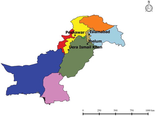
Site 1: Islamabad is the capital of Pakistan and the population has recently reached 1.017 million. The climate is subtropical with winter, spring, summer and autumn seasons. The average monsoon and annual precipitation is 790.8 and 1142.1 mm, respectively.

Site 2: Peshawar is the capital of Khyber Pakhtunkhwa (KP), with a population of 1.97 million in 2017. The climate in Peshawar is hot semi-arid, with hot summers and mild winters. The maximum PTCN in winter (236 mm) was recorded in February 2007 (PMD 2010, 2016), while a summer value of 402 mm was observed in July 2010.

Site 3: Jhelum is an agricultural district in Punjab, Pakistan. According to the census of 2017, the total population of Jhelum District is 1.22 million. The average rainfall of the area is about 1000 mm in the monsoon season (Department, 2010, PMD 2016). The main crops include wheat, pulses, bajra, maize, rice, fruits and vegetables.

Site 4: Dera Ismail Khan is situated in the province of Khyber Pakhtunkhwa, Pakistan, with a population of 1.6 million (2017 census). The climate of this area comprises scorching hot summers and mild winters, with an average annual precipitation of 268.8 mm/year. Water scarcity due to drought in 2012 severely affected the production of agricultural crops in this region (Amir 2012).

Some basic statistics and geographical information of the study areas, with the input predictors, are presented in Table 1. The selected regions are geographically diverse with both high (Site 1) and low elevation (Site 4).

Table 1. Descriptive statistics of the study sites with their climate data and climate indices over the study period (1981–2015). Site 1: Islamabad, Site 2: Peshawar, Site 3: Jhelum, and Site 4: Dera Ismail Khan. SD: standard deviation

	Climate data statistics
	Precipitation (mm)						Temperature (ºC)					Humidity (g/m^3)
Study site	Mean	Min	Max	SD	Skew	Kurt	Mean	Min	Max	SD	Skew	Kurt	Mean	Min	Max	SD	Skew	Kurt
Site 1	109.10	0.50	743.30	132.74	2.13	5.05	21.86	8.30	33.50	7.29	−0.22	−1.27	43.36	16.00	71.00	12.07	−0.06	−0.43
Site 2	45.79	1.00	409.00	52.16	2.85	12.64	23.09	9.30	81.10	8.69	1.20	7.20	45.36	19.00	69.70	10.54	−0.40	0.29
Site 3	75.66	0.20	648.60	96.12	2.50	8.42	23.75	10.50	34.90	7.16	−0.29	−1.13	46.15	15.00	77.00	13.29	−0.28	−0.49
Site 4	29.57	0.24	376.00	41.98	3.82	23.13	24.23	10.40	35.60	7.62	−0.29	−1.22	43.37	5.00	70.00	11.01	−0.36	0.28
Climate index statistics														Geographical characteristics
	Mean		Min		Max		SD			Skewness		Kurtosis		Study site		Longitude (ºE)	Latitude (ºN)	Elevation (m a.s.l.)
SOI	−1.49		−33.30		27.10		11.19			−0.13		−0.07
NINO3	25.90		23.06		29.21		1.30			−6.20		106.56
NINO3.4	27.07		24.48		29.23		1.01			−9.73		157.14		Site 1		73.08	33.73	604.00
NINO4	28.56		26.64		30.22		0.70			−14.39		210.18		Site 2		71.56	34.01	317.00
PDO	1.05		−2.33		184.00		14.68			11.77		139.17		Site 3		73.72	32.94	234.00
IOD	0.17		−0.70		1.54		0.32			0.60		1.69		Site 4		70.90	31.86	165.00
EMI	−0.08		−1.52		1.08		0.53			−0.55		−0.35
SAM	0.09		−3.25		4.92		1.10			0.08		1.41

3.2 Design of the multi-step NSGA-SVD-RF model

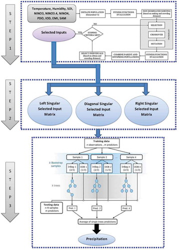
The proposed multi-step NSGA-SVD-RF model was established in MATLAB R2016b (The Math Works Inc. USA) with a Pentium 4 2.93 GHz dual core central processing unit. Historical climate data and synoptic climate mode indices lagged at (t – 1), (t – 2), (t – 3) were used in the first steps.

Step 1. The NSGA algorithm is used to determine the best input predictors (T, H, SOI, Niño3, Niño3.4, Niño4, PDO, IOD, EMI, SAM) for model development. The number of maximum iterations is 10, with population size 25 and mutation rate of 0.1. Further, the crossover percentage is 0.7% and a mutation percentage of 0.4% were used for each study site. The number of selected predictors for sites 1, 3 and 4 is two (Niño4, SAM), whereas in Site 2, seven predcitors were chosen (T, H, SOI, Niño3.4, Niño4, PDO, IOD) (see Table 2).

Table 2. Selected input predictors for each site using non-dominated sorting genetic algorithm of type II (NSGA). Ratio of selected inputs and root mean square error (RMSE) are also presented

Study site	Maximum iteration	Population size	Mutation rate	No. of selected input	Name of selected input	RMSE
Site 1	10	25	0.1	2	Niño4, SAM	119.93
Site 2	10	25	0.1	7	T, H, SOI, Niño3.4, Niño4, PDO, IOD	36.38
Site 3	10	25	0.1	2	Niño4, SAM	85.89
Site 4	10	25	0.1	2	Niño4, SAM	38.24

Step 2. The SVD method is used to decompsoe the selected input predictors of Step 1. The predefined parameters (i.e. no. of iterations and block size) used in the SVD model are presented in Table 3. The maximum number of iterations is three, with block size of two for each study site. The number of datum points for training and testing periods is also presented.

Table 3. Schematic statistics used in the singular value decomposition (SVD) method for the decomposition of selected input predictors for each site

Study site	No. of iterations	Block size	No. of training data points	No. of testing data points
Site 1	3	2	269	148
Site 2	3	2	269	148
Site 3	3	2	269	148
Site 4	3	2	269	148

The datasets are scaled within the range [0,1] to handle variances in skewness (Hsu et al. 2003). The normalization/scaling process is attained by (Hsu et al. 2003):

(8) ${\mathrm{\Theta }}_{\mathrm{n}\mathrm{o}\mathrm{r}\mathrm{m}}=\frac{\left(\mathrm{\Theta }-{\mathrm{\Theta }}_{\mathrm{m}\mathrm{i}\mathrm{n}}\right)}{\left({\mathrm{\Theta }}_{\mathrm{m}\mathrm{a}\mathrm{x}}-{\mathrm{\Theta }}_{\mathrm{m}\mathrm{i}\mathrm{n}}\right)}$(8)

where $\mathrm{\Theta }$ is the input/output, with min and max denoting the smallest and largest magnitudes of the data, and ${\mathrm{\Theta }}_{norm}$ is the desired normalized point. The datasets are divided into training data (70%) and testing data (30%) according to Cannas et al. (2006).

Step 3. After incorporating the historical input predictors at (t – 1) in the RF model, some predefined set of parameters such as the number of trees (10,000) and number of predictors (5) are selected through trial-and-hit method. The historical lags of t – 2 and t – 3 are also used in the developed model to obtain the optimum forecasting accuracy (see model M₃). The KRR model is also combined with the NSGA-SVD model to construct the NSGA-SVD-KRR model, and the standalone RF and KRR models are also evaluated. The NSGA-SVD-KRR and NSGA-KRR models use different types of kernels (Gaussian was the best in this study). Figure 2 gives a graphic representation of the NSGA-SVD-RF approach.

Figure 2. Detailed flow chart of the proposed multi-step non-sorting genetic algorithm of type-II (NSGA) integrated with singular value decomposition (SVD) and random forest – the NSGA-SVD-RF model

The training precision of the NSGA-SVD-RF model against benchmark models is evaluated using r and RMSE (Table 4).

3.4 Model assessment metrics

For PTCN forecasting, the performance of NSGA-SVD-RF and the benchmark comparison models was measured using the following statistical metrics: correlation coefficient (r), Willmott Index (WI), Nash-Sutcliffe efficiency coefficient (E_NS), root mean square error (RMSE, mm), mean absolute error (MAE, mm), the Legates and McCabe index (LM), and relative root mean square error (RRMSE, %), which are calculated as follows:

(9) $\text{eqalign{ \& {r !=!! {{{{{{cr \& left({eqalign{ \& {mathop sum nolimits }}^n\_{j = 1}left({{rm{PTC}}{{rm{N}}\_{{rm{OBS}}{,\_j}}}! - !!{ }{{overline {{rm{PTCN}}} }\_{{rm{OBS}}{,\_j}}}} right)}!cr \&left({{rm{PTC}}{{rm{N}}\_{{rm{FOR}}{,\_j}}}!! - {{overline {{rm{PTCN}}} }\_{{rm{FOR}}{,\_j}}}} right)}} over !{sqrt {{{left({{rm{PTC}}{{rm{N}}\_{{rm{OBS}}{,\_j}}}!! - {{overline {{rm{PTCN}}} }\_{{rm{OBS}}{,\_j}}}} right)}^2}}!! sqrt {{{left({{rm{PTC}}{{rm{N}}\_{{rm{FOR}}{,\_j}}}!! - {{overline {{rm{PTCN}}} }\_{{rm{FOR}}{,\_j}}}} right)}^2}} }}} right)}}$(9)

(10) $\text{r = left({{{{{mathop sum nolimits^ }^}\_{j = 1}^nleft({{rm{PTC}}{{rm{N}}\_{{rm{OBS}}{,\_j}}} - { }{{overline {{rm{PTCN}}} }\_{{rm{OBS}}{,\_j}}}} right)left({{rm{PTC}}{{rm{N}}\_{{rm{FOR}}{,\_j}}} - {{overline {{rm{PTCN}}} }\_{{rm{FOR}}{,\_j}}}} right)} over {sqrt {{{left({{rm{PTC}}{{rm{N}}\_{{rm{OBS}}{,\_j}}} - {{overline {{rm{PTCN}}} }\_{{rm{OBS}}{,\_j}}}} right)}^2}} sqrt {{{left({{rm{PTC}}{{rm{N}}\_{{rm{FOR}}{,\_j}}} - {{overline {{rm{PTCN}}} }\_{{rm{FOR}}{,\_j}}}} right)}^2}} }}} right)}$(10)

(11) $\text{{E\_{{rm{NS}}}} = 1 - left[{{{{{mathop sum nolimits^ }^}\_{j = 1}^n{{left({{rm{PTC}}{{rm{N}}\_{{rm{OBS}}{,\_j}}} - {rm{PTC}}{{rm{N}}\_{{rm{FOR}}{,\_j}}}} right)}^2}} over {{{mathop sum nolimits^ }^}\_{j = 1}^1{{left({{rm{PTC}}{{rm{N}}\_{{rm{OBS}}{,\_j}}} - { }{{overline {{rm{PTCN}}} }\_{{rm{FOR}}{,\_j}}}} right)}^2}}}} right], - infty le {E\_{{rm{NS}}}} le 1}$(11)

(12) $\mathrm{R}\mathrm{M}\mathrm{S}\mathrm{E}=\sqrt{\frac{1}{n}}{\sum }_{j=1}^1{\left(\mathrm{P}\mathrm{T}\mathrm{C}{\mathrm{N}}_{\mathrm{F}\mathrm{O}\mathrm{R}{,}_j}-\mathrm{P}\mathrm{T}\mathrm{C}{\mathrm{N}}_{\mathrm{O}\mathrm{B}\mathrm{S}{,}_j}\right)}^2$(12)

(13) $\mathrm{R}\mathrm{M}\mathrm{S}\mathrm{E}=\sqrt{\frac{1}{n}}{\sum }_{j=1}^1{\left(\mathrm{P}\mathrm{T}\mathrm{C}{\mathrm{N}}_{\mathrm{F}\mathrm{O}\mathrm{R}{,}_j}-\mathrm{P}\mathrm{T}\mathrm{C}{\mathrm{N}}_{\mathrm{O}\mathrm{B}\mathrm{S}{,}_j}\right)}^2$(13)

(14) $\text{{rm{LM}} = 1 - left[{{{{{mathop sum nolimits^ }^}\_{j = 1}^nleft| {{rm{PTC}}{{rm{N}}\_{{rm{FOR}}{,\_j}}} - {rm{PTC}}{{rm{N}}\_{{rm{OBS}}{,\_j}}}} right|} over {{{mathop sum nolimits^ }^}\_{j = 1}^nleft| {{rm{PTC}}{{rm{N}}\_{{rm{OBS}}{,\_j}}} - {{overline {{rm{PTCN}}} }\_{{rm{OBS}}{,\_j}}}} right|}}} right],{ }0 le LM le 1}$(14)

(15) $\text{{rm{LM}} = 1 - left[{{{{{mathop sum nolimits^ }^}\_{j = 1}^nleft| {{rm{PTC}}{{rm{N}}\_{{rm{FOR}}{,\_j}}} - {rm{PTC}}{{rm{N}}\_{{rm{OBS}}{,\_j}}}} right|} over {{{mathop sum nolimits^ }^}\_{j = 1}^nleft| {{rm{PTC}}{{rm{N}}\_{{rm{OBS}}{,\_j}}} - {{overline {{rm{PTCN}}} }\_{{rm{OBS}}{,\_j}}}} right|}}} right],{ }0 le LM le 1}$(15)

where $\mathrm{P}\mathrm{T}\mathrm{C}{\mathrm{N}}_{\mathrm{O}\mathrm{B}\mathrm{S}{,}_j}$ and $\mathrm{P}\mathrm{T}\mathrm{C}{\mathrm{N}}_{\mathrm{O}\mathrm{B}\mathrm{S}{,}_j}$ are the observed and forecasted jth magnitude of monthly precipitation, PTCN; ${\overline{\mathrm{P}\mathrm{T}\mathrm{C}\mathrm{N}}}_{\mathrm{O}\mathrm{B}\mathrm{S}{,}_j}$and ${\overline{\mathrm{P}\mathrm{T}\mathrm{C}\mathrm{N}}}_{\mathrm{O}\mathrm{B}\mathrm{S}{,}_j}$ are the observed and forecasted average of PTCN; and n is the total number of tested data points.

4 Results

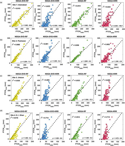
The NSGA-SVD-RF model clearly exhibits a better accuracy than NSGA-SVD-KRR, NSGA-RF and NSGA-KRR models in terms of r² (NSGA-SVD-RF: 0.915, NSGA-SVD-KRR: 0.633, NSGA-RF: 0.914, NSGA-KRR: 0.633) for Site 1, as shown in the scatterplot in Fig. 3. Similarly, the proposed multi-step NSGA-SVD-RF model is more accurate for Site 2 in terms of r² values (NSGA-SVD-RF: 0.960, NSGA-SVD-KRR: 0.861, NSGA-RF: 0.956, NSGA-KRR: 0.802). The NSGA-SVD-RF model for sites 3 and 4 is reasonably good compared to the NSGA-SVD-KRR, NSGA-RF and NSGA-KRR models (Fig. 3). The improved accuracy of the proposed multi-step NSGA-SVD-RF model is confirmed against the comparison models in terms of r² value.

Figure 3. Scatterplot of the monthly forecasted and observed precipitation (PTCN_FOR and PTCN_OBS) (mm) in the testing phase for the proposed multi-step NSGA-SVD-RF, NSGA-SVD-KRR, NSGA-RF and NSGA-KRR models using the coefficient of determination (r²) and a linear fit inserted in each panel for (a) Site 1: Islamabad, (b) Site 2: Peshawar, (c) Site 3: Jhelum, and (d) Site 4: D. I. Khan

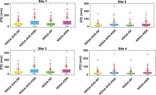
Figure 4 compares boxplots of NSGA-SVD-RF model with those of the comparison models. The distributed |FE| error is confirmed with a much smaller quartile and was assimilated by the proposed multi-step NSGA-SVD-RF model for sites 2 and 4, followed by the NSGA-RF, NSGA-SVD-KRR and NSGA-KRR models. The NSGA-SVD-RF acquired a better precision for sites 1 and 3. By analysing Fig. 4, the accuracy of NSGA-SVD-RF model appeared reasonably good for all sites.

Figure 4. Boxplots of the monthly forecasted error |FE| (mm) between forecasted and observed PTCN in the testing period of the proposed multi-step NSGA-SVD-RF model vs the NSGA-SVD-KRR, NSGA-RF and NSGA-KRR models for Site 1: Islamabad, Site 2: Peshawar, Site 3: Jhelum, and Site 4: D. I. Khan

In Table 5, the precision of NSGA-SVD-RF is appraised against comparison models through r, RMSE and MAE. The NSGA-SVD-RF model at Site 1 attained the maximum r (0.947) and minimum RMSE (60.26 mm) and MAE (44.17 mm) as compared to the NSGA-SVD-KRR model (r = 0.741, RMSE = 100.56 mm, MAE = 75.39 mm), the NSGA-RF model (r = 0.946, RMSE = 60.74 mm, MAE = 44.28 mm) and the NSGA-KRR model (r = 0.741, RMSE = 100.55 mm, MAE = 75.39 mm). Similarly, the efficiency of the NSGA-SVD-RF model is improved for sites 2, 3 and 4 by accomplishing the largest r and smallest RMSE and MAE values (Table 5). This is a strong sign that the NSGA-SVD-RF model is a healthier data-intelligent approach to forecast PTCN.

Table 4. Training performance of the multi-step NSGA-SVD-RF model vs the NSGA-SVD-KRR, NSGA-RF and NSGA-KRR models between monthly forecasted and observed precipitation in terms of correlation coefficient (r) and root mean square error (RMSE, mm). Bold indicates the best model

Model	Historical lag	NSGA-SVD-RF				NSGA-SVD-KRR			NSGA-RF				NSGA-KRR
				Training period		Kernel	Training period			No. of predictor split	Training period		Kernel	Training period
		No. of trees	No. of predictor split	RMSE (mm)	r		RMSE (mm)	r	No. of trees		RMSE (mm)	r		RMSE (mm)	r
Site 1
M1	(t – 1)	10,000	100	66.40	0.937	Gaussian	121.70	0.425	10,000	100	69.36	0.924	Gaussian	121.70	0.425
M2	(t – 1) + (t – 2)	10,000	100	64.55	0.955	Gaussian	113.77	0.615	10,000	100	65.07	0.954	Gaussian	113.77	0.615
M3	(t – 1) + (t – 2) + (t – 3)	10,000	100	62.21	0.963	Gaussian	111.25	0.693	10,000	100	62.79	0.962	Gaussian	111.25	0.693
Site 2
M1	(t – 1)	10,000	100	18.44	0.951	Gaussian	15.85	0.964	10,000	100	17.90	0.961	Gaussian	15.85	0.964
M2	(t – 1) + (t – 2)	10,000	100	17.40	0.961	Gaussian	15.85	0.964	10,000	100	16.28	0.964	Gaussian	15.85	0.964
M3	(t – 1) + (t – 2) + (t – 3)	10,000	100	16.97	0.960	Gaussian	15.85	0.964	10,000	100	15.85	0.964	Gaussian	15.85	0.964
Site 3
M1	(t – 1)	10,000	100	50.36	0.929	Gaussian	46.74	0.959	10,000	100	52.28	0.918	Gaussian	46.74	0.959
M2	(t – 1) + (t – 2)	10,000	100	48.72	0.951	Gaussian	46.74	0.959	10,000	100	49.39	0.948	Gaussian	46.74	0.959
M3	(t – 1) + (t – 2) + (t – 3)	10,000	100	46.19	0.961	Gaussian	46.74	0.959	10,000	100	46.74	0.959	Gaussian	46.74	0.959
Site 4
M1	(t – 1)	10,000	100	16.02	0.935	Gaussian	14.48	0.966	10,000	100	16.52	0.925	Gaussian	14.48	0.966
M2	(t – 1) + (t – 2)	10,000	100	15.31	0.956	Gaussian	14.48	0.966	10,000	100	15.57	0.953	Gaussian	14.48	0.966
M3	(t – 1) + (t – 2) + (t – 3)	10,000	100	14.35	0.968	Gaussian	14.48	0.966	10,000	100	14.48	0.966	Gaussian	14.48	0.966

Table 5. Testing performance of the NSGA-SVD-RF model vs the NSGA-SVD-KRR, NSGA-RF and NSGA-KRR models measured by root mean square error (RMSE, mm), mean absolute error (MAE, mm), correlation coefficient (r) between monthly forecasted and observed precipitation. Bold indicates the best model

Model	Lags	NSGA-SVD-RF			NSGA-SVD-KRR			NSGA-RF				NSGA-KRR
			RMSE (mm)	MAE (mm)	r	RMSE (mm)	MAE (mm)	r	RMSE (mm)	MAE (mm)	r	RMSE (mm)	MAE (mm)	r
Site 1
M1	(t – 1),		67.20	49.35	0.900	112.04	84.38	0.525	68.39	50.29	0.894	112.04	84.38	0.525
M2	(t – 1), (t – 2)		64.35	47.26	0.933	104.31	78.49	0.671	64.92	47.71	0.931	104.30	78.49	0.671
M3	(t – 1), (t – 2), (t – 3)		60.26	44.17	0.947	100.56	75.39	0.741	60.74	44.28	0.946	100.55	75.39	0.741
Site 2
M1	(t – 1),		25.97	17.68	0.946	47.06	32.30	0.685	27.26	17.64	0.962	45.11	30.51	0.770
M2	(t – 1), (t – 2)		24.57	16.10	0.956	43.11	28.96	0.794	25.42	16.39	0.969	41.05	27.63	0.854
M3	(t – 1), (t – 2), (t – 3)		23.52	14.92	0.962	40.97	27.25	0.838	24.60	15.45	0.968	34.52	23.46	0.823
Site 3
M1	(t – 1),		42.76	31.55	0.917	73.89	54.18	0.497	43.24	31.92	0.915	73.89	54.18	0.497
M2	(t – 1), (t – 2)		42.17	30.22	0.932	68.66	50.05	0.625	42.44	30.40	0.931	68.65	50.05	0.625
M3	(t – 1), (t – 2), (t – 3)		38.15	27.12	0.953	63.89	46.85	0.722	38.56	27.36	0.950	63.88	46.85	0.722
Site 4
M1	(t – 1),		28.24	18.12	0.882	43.61	29.44	0.539	28.34	18.27	0.881	43.62	29.44	0.539
M2	(t – 1), (t – 2)		26.52	17.54	0.932	40.57	27.57	0.692	26.80	17.76	0.932	40.14	27.33	0.702
M3	(t – 1), (t – 2), (t – 3)		25.46	16.47	0.941	38.97	26.25	0.769	25.68	16.67	0.938	38.97	26.25	0.769

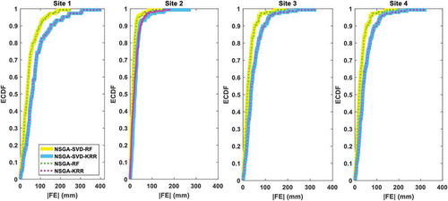
The empirical cumulative distribution function (ecdf) in Fig. 5 portrays the different predicting skills. The NSGA-SVD-RF model was superior to the comparative models NSGA-SVD-KRR, NSGA-RF and NSGA-KRR. Based on the error (0 to ±400 mm) for all study sites, Fig. 5 clearly shows that the proposed multi-step NSGA-SVD-RF model is a precise model.

Figure 5. Empirical cumulative distribution function (ecdf) of the monthly forecasted error |FE| (mm) between forecasted and observed PTCN generated by the proposed multi-step NSGA-SVD-RF model vs the NSGA-SVD-KRR, NSGA-RF and NSGA-KRR models for Site 1: Islamabad, Site 2: Peshawar, Site 3: Jhelum, and Site 4: D. I. Khan

Table 6 describes the performance of the NSGA-SVD-RF model in comparison with the NSGA-SVD-KRR, NSGA-RF and NSGA-KRR models, evaluated for all sites in terms of WI, E_NS and LM. The proposed multi-step NSGA-SVD-RF model in Site 1 attained the highest values of WI (0.712), E_NS (0.774) and LM (0.541) and was followed by the NSGA-SVD-KRR (WI = 0.294, E_NS = 0.371 and LM = 0.216), the NSGA-RF model (WI = 0.710, E_NS = 0.770 and LM = 0.540) and the NSGA-KRR model (WI = 0.294, E_NS = 0.371 and LM = 0.216). For sites 2, 3 and 4, the proposed model again appears to be the best as compared to the comparison models (see Table 6).

Table 6. Performance of the proposed multi-step NSGA-SVD-RF model vs the NSGA-SVD-KRR, NSGA-RF and NSGA-KRR models using the Willmott index (WI), the Nash-Sutcliffe efficiency (E_NS) and the Legates-McCabe index (LM) in the testing period. Bold indicates the best model

Model	Lag	NSGA-SVD-RF			NSGA-SVD-KRR			NSGA-RF			NSGA-KRR
		WI	ENS	LM	WI	ENS	LM	WI	ENS	LM	WI	ENS	LM
Site 1
M1	(t – 1)	0.667	0.720	0.494	0.196	0.223	0.136	0.657	0.710	0.485	0.196	0.223	0.136
M2	(t – 1), (t – 2)	0.683	0.743	0.512	0.268	0.324	0.190	0.677	0.738	0.508	0.268	0.324	0.190
M3	(t – 1), (t – 2), (t – 3)	0.712	0.774	0.541	0.294	0.371	0.216	0.710	0.770	0.540	0.294	0.371	0.216
Site 2
M1	(t – 1)	0.754	0.811	0.579	0.312	0.380	0.230	0.722	0.792	0.580	0.348	0.430	0.273
M2	(t – 1), (t – 2)	0.771	0.829	0.611	0.385	0.473	0.300	0.749	0.817	0.604	0.424	0.522	0.332
M3	(t – 1), (t – 2), (t – 3)	0.790	0.843	0.637	0.431	0.524	0.337	0.765	0.828	0.624	0.621	0.662	0.429
Site 3
M1	(t – 1)	0.665	0.735	0.488	0.185	0.209	0.121	0.661	0.729	0.482	0.185	0.209	0.121
M2	(t – 1), (t – 2)	0.662	0.738	0.502	0.249	0.306	0.175	0.660	0.735	0.499	0.249	0.306	0.175
M3	(t – 1), (t – 2), (t – 3)	0.709	0.781	0.544	0.302	0.385	0.212	0.705	0.776	0.540	0.302	0.385	0.212
Site 4
M1	(t – 1)	0.520	0.667	0.436	0.103	0.206	0.084	0.520	0.665	0.432	0.103	0.206	0.084
M2	(t – 1), (t – 2)	0.554	0.708	0.456	0.179	0.317	0.145	0.550	0.704	0.451	0.187	0.332	0.153
M3	(t – 1), (t – 2), (t – 3)	0.581	0.731	0.486	0.212	0.370	0.180	0.574	0.727	0.479	0.212	0.370	0.180

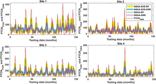
Figure 6 plots the time series comparison of the monthly forecasted PTCN, generated by the multi-step NSGA-SVD-RF model together with the NSGA-SVD-KRR, NSGA-RF and NSGA-KRR models in the testing period. Moreover, the forecasted PTCN is also plotted in comparison with the observed PTCN. There is compelling evidence that the well-tuned NSGA-SVD-RF model performs accurately for all sites, in comparison to the counterpart models.

Figure 6. Time series of the monthly forecasted and observed PTCN in the testing period using the proposed multi-step NSGA-SVD-RF model vs the NSGA-SVD-KRR, NSGA-RF and NSGA-KRR models for Site 1: Islamabad, Site 2: Peshawar, Site 3: Jhelum, and Site 4: D. I. Khan

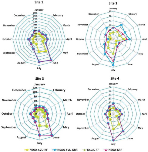
Figure 7 presents the average |FE| error yield for January–December for each site. The |FE| error generated by the proposed multi-step NSGA-SVD-RF and NSGA-RF models was very low compared to the NSGA-SVD-KRR and NSGA-KRR models for all sites. The |FE| error was significantly smaller in all months except June and July for the proposed multi-step NSGA-SVD-RF and NSGA-RF models as compared to the NSGA-SVD-KRR and NSGA-KRR models in sites 1, 3 and 4, while for July and August, the |FE| error was slightly higher than other months for these models. Overall, the proposed model generated significant accuracy with smaller error statistics.

Figure 7. Polar plots showing the average monthly values of the monthly forecasted error |FE| (mm) between forecasted and observed PTCN in the testing period using the proposed multi-step NSGA-SVD-RF model vs the NSGA-SVD-KRR, NSGA-RF and NSGA-KRR models for Site 1: Islamabad, Site 2: Peshawar, Site 3: Jhelum, and Site 4: D. I. Khan

Table 7 shows the relative root mean squared error (RRMSE) in terms of the percentage error for the four sites. On the basis of RRMSE, Site 2 seems to be the most precise station in forecasting PTCN where the NSGA-SVD-RF model performed the best (RRMSE = 43.43%) followed by Site 1 (53.31%), Site 3 (53.58%) and Site 4 (74.08%). The proposed multi-step NSGA-SVD-RF model shows a good accuracy by generating the lowest RRMSE errors.

Table 7. Geographical comparison of the accuracy of the NSGA-SVD-RF model vs the NSGA-SVD-KRR, NSGA-RF and NSGA-KRR models in terms of relative root mean squared error (RRMSE, %) computed within the test sites. Bold indicates the best model

Model	Lag	NSGA-SVD-RF	NSGA-SVD-KRR	NSGA-RF	NSGA-KRR
		RRMSE (%)	RRMSE (%)	RRMSE (%)	RRMSE (%)
Site 1
M1	(t – 1)	58.41	97.38	59.45	97.38
M2	(t – 1), (t – 2)	56.43	91.47	56.93	91.47
M3	(t – 1), (t – 2), (t – 3)	53.31	88.96	53.73	88.95
Site 2
M1	(t – 1)	47.02	85.22	49.36	81.68
M2	(t – 1), (t – 2)	45.04	79.03	46.60	75.25
M3	(t – 1), (t – 2), (t – 3)	43.43	75.66	45.43	63.75
Site 3
M1	(t – 1)	58.27	100.69	58.92	100.69
M2	(t – 1), (t – 2)	58.28	94.88	58.65	94.87
M3	(t – 1), (t – 2), (t – 3)	53.58	89.74	54.17	89.73
Site 4
M1	(t – 1)	81.24	125.45	81.51	125.45
M2	(t – 1), (t – 2)	76.45	116.94	77.05	115.70
M3	(t – 1), (t – 2), (t – 3)	74.08	113.38	74.70	113.38

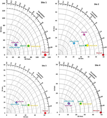
Figure 8 shows a Taylor diagram for a more solid and certain performance based on the statistical observation on the basis of correlation coefficient (r) and standard deviation. For Site 1, the r value of the NSGA-SVD-RF model with observations was about 0.96, followed by the NSGA-RF model (0.95), and the NSGA-SVD-KRR and NSGA-KRR models (0.80). The proposed multi-step NSGA-SVD-RF model was nearer to the observed PTCN for sites 2, 3 and 4. Overall, the correlation, r of the proposed multi-step NSGA-SVD-RF model was better than the other compared models.

Figure 8. Taylor diagram showing the correlation coefficient between the monthly forecasted and observed PTCN (mm) and standard deviation for the proposed multi-step NSGA-SVD-RF model in comparison with the NSGA-SVD-KRR, NSGA-RF and NSGA-KRR models for Site 1: Islamabad, Site 2: Peshawar, Site 3: Jhelum, and Site 4: D. I. Khan

5 Discussion

In this study, we designed a multi-step NSGA-SVD-RF model using climate data and synoptic climate indices to forecast monthly precipitation in Pakistan at four sites that each experience different annual climate patterns. The model used the NSGA algorithm for input selection in a first step, while the SVD algorithm further decomposed the selected input in the second step. Finally, the RF model was applied to forecast PTCN. The proposed NSGA-SVD-RF model was compared with NSGA-SVD-KRR, NSGA-RF and NSGA-KRR models.

The developed NSGA-SVD-RF model was effectively appraised to generate smaller relative percentage errors in terms of RRMSE and r, WI, E_NS (Tables 5-7). The performance was high, according to the achieved assessment criteria used (Equations (6)(6) $\mathrm{\Psi }\left(,z_l,z_s\right)={\left(z_l^T.z_s+R\right)}^D$(6) –(12(12) $\mathrm{R}\mathrm{M}\mathrm{S}\mathrm{E}=\sqrt{\frac{1}{n}}{\sum }_{j=1}^1{\left(\mathrm{P}\mathrm{T}\mathrm{C}{\mathrm{N}}_{\mathrm{F}\mathrm{O}\mathrm{R}{,}_j}-\mathrm{P}\mathrm{T}\mathrm{C}{\mathrm{N}}_{\mathrm{O}\mathrm{B}\mathrm{S}{,}_j}\right)}^2$(12) )). Thus, the proposed multi-step NSGA-SVD-RF model can be adopted for long-term PTCN forecasting where the forecasting of future PTCN from standard meteorological and climate parameters will likely become more important due to climate change and an increase in water demand.

Accurate PTCN forecasting and developing early warning systems can have numerous benefits, both nationally and internationally (Palmer 1965, Langridge et al. 2006, Barredo 2007, Vörösmarty et al. 2010). Accurate PTCN forecasting can play an important role in the aforementioned situation for both developed and under-developing nations such as Pakistan. Further, this study can be adopted anywhere for PTCN forecasting using the universally synoptic climate mode indices as input predictors. The proposed multi-step NSGA-SVD-RF model can be applied for agriculture crop yield prediction which could be of interest to the government’s national policy-making and agricultural engineers to help minimize crop estimation uncertainties (Akhtar 2014, Niaz 2014).

It is noted that this study utilized the historical climate data and synoptic climate mode indices to forecast PTCN and therefore, carries some limitations. To enhance the scope of this study, other atmospheric data such as cloud cover, sunshine and air temperatures, soil moisture, solar radiation etc. could also be used to forecast PTCN. Such predictor variables (whose data could be remotely sensed through satellites or atmospheric simulation models) (e.g. (Bauer 1975, Stathakis et al. 2006, Chen and Mcnairn 2006, Dempewolf et al. 2014, Kumar et al. 2015)) are likely to be greatly valued for modelling PTCN in remotely located zones. Further, as processed based modelling is resource demanding and cost-prohibitive for developing countries, the proposed multi-step NSGA-SVD-RF model may be seen as a viable solution. Moreover, as the proposed approach utilized synoptic climate mode indices, it can be applied in those regions where meteorological data are not available.

The proposed multi-step NSGA-SVD-RF model could be improved by an ensemble approach to possibly achieve more accurate results. New advanced optimization techniques could comprise: Quantum-Behaved PSO and the Firefly Algorithm to select input predictors which have been tested to hybridize with the RF and other models (e.g. (Sedki and Ouazar 2010, Pal et al. 2012, Hoang et al. 2014, Kayarvizhy et al. 2014, Taormina and Chau 2015, Taormina et al. 2015, Raheli et al. 2017, Ghorbani et al. 2018)). Further, empirical wavelet transform (Gilles 2013) and empirical mode composition (Huang et al. 1998) may be additional approaches. Copula modelling (Nguyen-Huy et al. 2017) can be applied in terms of statistical approaches where joint behaviour of multivariate data (e.g. PTCN and corresponding predictors) can be modelled.

6 Conclusion

This research has designed a multi-step NSGA-SVD-RF model using climate data and synoptic climate mode indices to forecast precipitation (PTCN). The PTCN data from 1981 to 2015 were incorporated to determine the best-inputs by the NSGA algorithm. The selected inputs were then incorporated in the SVD method to decompose them in the second step and finally the historical lags of the selected decomposed data at (t-1), (t-2) and (t-3) were inserted in the RF model to design the optimum NSGA-SVD-RF model. Further, Distinctive assessment criterion were used to gauge the performance of NSGA-SVD-RF model.

The NSGA-SVD-RF model was compared with NSGA-SVD-KRR, NSGA-RF and NSGA-KRR models. As evident by small relative |FE| errors and large assessing metrics, the accuracy of NSGA-SVD-RF model is much better than that of counterpart models. Because the feature selection done by NSGA and then decomposing the selected features by SVD enables the proposed multi-step model to optimize enough to obtained better accuracy. The selection of relevant features (i.e. predictors) is very important because it is the unnecessary variables the leads the models to poor performance. Therefore, the proposed multi-step NSGA-SVD-RF model is a more refined and filtered technique to forecast future precipitation. The |FE| errors for the best site 2 achieved by the proposed multi-step NSGA-SVD-RF model were RMSE ≈ 43.43%. In terms of normalized performance metrics, their magnitudes for site 2 were r ≈ 0.962, WI ≈ 0.790 and NS_E ≈ 0.843 (Tables 5 and 6).

The performance of NSGA-SVD-RF hybrid model in relation to their counterpart models on the basis of LM was superior. The acquired LM for study site 2 were LM ≈ 0.637 (NSGA-SVD-RF), 0.337 (NSGA-SVD-KRR), 0.624 (NSGA-RF) and 0.429 (NSGA-KRR) respectively. Further, a reasonable degree of geographic variability was apparent through RRMSE with the optimal performance acquired for site 2 as compared to other sites 1, 3 & 4. Finally, this study provides a new data-driven approach where both the climate input data and large-scale climate mode indices may be incorporated to forecast precipitation in any region a reasonable correlation between these variables exist and where agricultural and other socio-economic activities require a management of water resources to help hydrologists and agricultural managers in key long-term decisions.

Acknowledgements

The dataset attained from Pakistan Meteorological Department, Pakistan and the authors are duly acknowledge the Pakistan Meteorological Department.

Disclosure statement

No potential conflict of interest was reported by the authors.

Additional information

Funding

Financial funding is not available for this research work; University of Southern Queensland [USQPRS Scholarship 2017-2019];

References

- Aamir, E. and Hassan, I., 2018. Trend analysis in precipitation at individual and regional levels in Baluchistan, Pakistan. IOP Conference Series: Materials Science and Engineering. Bristol, UK: IOP Publishing, p. 012042.
- Akhtar, I.U.H., 2014. Pakistan needs a new crop forecasting system. Available from: https://www.scidev.net/global/climate-change/opinion/pakistan-needs-a-new-crop-forecasting-system.html
- Alaoui, A. and Mahoney, M.W., 2015. Fast randomized kernel ridge regression with statistical guarantees. Advances in Neural Information Processing Systems, 775–783.
- Ali, M., et al., 2018a. An ensemble-ANFIS based uncertainty assessment model for forecasting multi-scalar standardized precipitation index. Atmospheric Research, 207, 155–180. doi:10.1016/j.atmosres.2018.02.024
- Ali, M., et al., 2018b. Multi-stage hybridized online sequential extreme learning machine integrated with Markov Chain Monte Carlo copula-Bat algorithm for rainfall forecasting. Atmospheric Research, 213, 450–464. doi:10.1016/j.atmosres.2018.07.005
- Ali, M., et al., 2020. Complete ensemble empirical mode decomposition hybridized with random forest and kernel ridge regression model for monthly rainfall forecasts. Journal of Hydrology, 584, 124647.
- Alter, O., Brown, P.O., and Botstein, D., 2000. Singular value decomposition for genome-wide expression data processing and modeling. Proceedings of the National Academy of Sciences, 97, 10101–10106. doi:10.1073/pnas.97.18.10101
- Amir, I., 2012. Tough times ahead for farmers in southern KP. DAWN. Available from: https://www.dawn.com/news/698605/tough-times-ahead-for-farmers-in-southern-kp
- Archer, D.R. and Fowler, H.J., 2008. Using meteorological data to forecast seasonal runoff on the River Jhelum, Pakistan. Journal of Hydrology, 361, 10–23. doi:10.1016/j.jhydrol.2008.07.017
- Barredo, J.I., 2007. Major flood disasters in Europe: 1950–2005. Natural Hazards, 42, 125–148. doi:10.1007/s11069-006-9065-2
- BAS, 2018. British Antarctic survey [Online]. Available from: http://www.atmos.colostate.edu/~davet/ao/Data/ [accessed 21 October 2020].
- Bauer, M.E., 1975. The role of remote sensing in determining the distribution and yield of crops. Advances in Agronomy, 27, 271–304.
- Bhalme, H.N. and Mooley, D.A., 1980. Large-scale droughts/floods and monsoon circulation. Monthly Weather Review, 108, 1197–1211. doi:10.1175/1520-0493(1980)108<1197:LSDAMC>2.0.CO;2
- Breiman, L., 1996. Bagging predictors. Machine Learning, 24, 123–140. doi:10.1007/BF00058655
- Breiman, L., 2001. Random forests. Machine Learning, 45, 5–32. doi:10.1023/A:1010933404324
- Bretherton, C.S., Smith, C., and Wallace, J.M., 1992. An intercomparison of methods for finding coupled patterns in climate data. Journal of Climate, 5, 541–560. doi:10.1175/1520-0442(1992)005<0541:AIOMFF>2.0.CO;2
- Burlando, P., et al., 1993. Forecasting of short-term rainfall using ARMA models. Journal of Hydrology, 144, 193–211. doi:10.1016/0022-1694(93)90172-6
- Cannas, B., et al., 2006. Data preprocessing for river flow forecasting using neural networks: wavelet transforms and data partitioning. Physics and Chemistry of the Earth, Parts A/B/C, 31, 1164–1171. doi:10.1016/j.pce.2006.03.020
- Cao, L., 2006. Singular value decomposition applied to digital image processing. In: Division of Computing Studies, Arizona State University Polytechnic Campus, Mesa, Arizona State University polytechnic Campus, 1–15. Available from: https://www.math.cuhk.edu.hk/~lmlui/CaoSVDintro.pdf
- Chen, C. and Mcnairn, H., 2006. A neural network integrated approach for rice crop monitoring. International Journal of Remote Sensing, 27 (7), 1367–1393. doi:10.1080/01431160500421507
- Chen, J., Li, M., and Wang, W., 2012. Statistical uncertainty estimation using random forests and its application to drought forecast. Mathematical Problems in Engineering. doi:10.1155/2012/915053
- Chiew, F.H., et al., 1998. El Niño/Southern oscillation and Australian rainfall, streamflow and drought: links and potential for forecasting. Journal of Hydrology, 204, 138–149. doi:10.1016/S0022-1694(97)00121-2
- Chiew, F.H. and Mcmahon, T.A., 2002. Modelling the impacts of climate change on Australian streamflow. Hydrological Processes, 16, 1235–1245. doi:10.1002/hyp.1059
- Choubin, B., et al., 2014. Drought forecasting in a semi-arid watershed using climate signals: a neuro-fuzzy modeling approach. Journal of Mountain Science, 11, 1593–1605. doi:10.1007/s11629-014-3020-6
- Choubin, B., et al., 2017. An ensemble forecast of semi‐arid rainfall using large‐scale climate predictors. Meteorological Applications, 24, 376–386. doi:10.1002/met.1635
- Choubin, B., et al., 2018. Precipitation forecasting using classification and regression trees (CART) model: a comparative study of different approaches. Environmental Earth Sciences, 77 (8), 314. doi:10.1007/s12665-018-7498-z
- Choubin, B., et al., 2019. Effects of large-scale climate signals on snow cover in Khersan watershed, Iran. Extreme Hydrology and Climate Variability.
- Choubin, B., Malekian, A., and Gloshan, M., 2016. Application of several data-driven techniques to predict a standardized precipitation index. Atmósfera, 29, 121–128. doi:10.20937/ATM.2016.29.02.02
- Cong, F., et al., 2013. Short-time matrix series based singular value decomposition for rolling bearing fault diagnosis. Mechanical Systems and Signal Processing, 34, 218–230. doi:10.1016/j.ymssp.2012.06.005
- Danaher, S., et al., 1997. A comparison of the characterisation of agricultural land using singular value decomposition and neural networks. In: I. Kanellopoulos, G.G. Wilkinson, F. Roli, J. Austin, eds. Neurocomputation in Remote Sensing Data Analysis. Berlin, Heidelberg: Springer. doi:10.1007/978-3-642-59041-2_3
- De Jong, K.A., 1975. Analysis of the behavior of a class of genetic adaptive systems. Ann Arbor, USA: University of Michigan Dept.
- Deb, K., et al., 2002. A fast and elitist multiobjective genetic algorithm: NSGA-II. IEEE Transactions on Evolutionary Computation, 6, 182–197. doi:10.1109/4235.996017
- Dempewolf, J., et al., 2014. Wheat yield forecasting for Punjab Province from vegetation index time series and historic crop statistics. Remote Sensing, 6, 9653–9675. doi:10.3390/rs6109653
- Deo, R. and Şahin, M., 2015. Application of the artificial neural network model for prediction of monthly standardized precipitation and evapotranspiration index using hydrometeorological parameters and climate indices in eastern Australia. Atmospheric Research, 161-162, 65–81. doi:10.1016/j.atmosres.2015.03.018
- Deo, R. and Şahin, M., 2016. An extreme learning machine model for the simulation of monthly mean streamflow water level in eastern Queensland. Environmental Monitoring and Assessment, 188, 90. doi:10.1007/s10661-016-5094-9.
- Deo, R.C., Kisi, O., and Singh, V.P., 2017. Drought forecasting in eastern Australia using multivariate adaptive regression spline, least square support vector machine and M5Tree model. Atmospheric Research, 184, 149–175. doi:10.1016/j.atmosres.2016.10.004
- Department P. M. 2010. Dry weather predicted in the country during Friday/Monday [Online]. Available from: https://web.archive.org/web/20100902112830/http://www.pakmet.com.pk/latest%20news/Latest%20News.html [accessed 21 October 2020].
- Drosdowsky, W., 1993. An analysis of Australian seasonal rainfall anomalies: 1950–1987. II: temporal variability and teleconnection patterns. International Journal of Climatology, 13, 111–149. doi:10.1002/joc.3370130202
- Ghorbani, M.A., et al., 2018. Pan evaporation prediction using a hybrid multilayer perceptron-firefly algorithm (MLP-FFA) model: case study in North Iran. Theoretical and Applied Climatology 3, 1119–31. doi:10.1007/s00704-017-2244-0
- Gilles, J., 2013. Empirical wavelet transform. IEEE Transactions on Signal Processing, 61, 3999–4010. doi:10.1109/TSP.2013.2265222
- Golchha, A. and QURESHI, S.G., 2015. Non-dominated sorting genetic algorithm-II–a succinct survey. International Journal of Computer Science and Information Technologies, 6, 252–255.
- Herries, G., Selige, T., and Danaher, S., 1996. Singular value decomposition in applied remote sensing. In: IEE Colloquium on Image Processing for Remote Sensing. London, UK, 5/1–5/6. doi:10.1049/ic:19960159
- Hoang, N.-D., Pham, A.-D., and Cao, M.-T., 2014. A novel time series prediction approach based on a hybridization of least squares support vector regression and swarm intelligence. Applied Computational Intelligence and Soft Computing, 2014, 15. doi:10.1155/2014/754809
- Hsu, C.-W., Chang, -C.-C., and Lin, C.-J., 2003. A practical guide to support vector classification. Available from: https://www.csie.ntu.edu.tw/~cjlin/papers/guide/guide.pdf [accessed 21 October 2020].
- Huang, N.E., et al., 1998. The empirical mode decomposition and the Hilbert spectrum for nonlinear and non-stationary time series analysis. Proceedings of the Royal Society of London A: Mathematical, Physical and Engineering Sciences. The Royal Society, 903–995. doi:10.1098/rspa.1998.0193
- Hung, N.Q., et al., 2009. An artificial neural network model for rainfall forecasting in Bangkok, Thailand. Hydrology and Earth System Sciences, 13, 1413–1425. doi:10.5194/hess-13-1413-2009
- JAMSTEC, 2018. Japan agency for marine-earth science [Online]. Japan Agency for Marine-Earth Science.
- JISAO, 2018. Joint institute of the study of the atmosphere and ocean [Online]. Available from: http://research.jisao.washington.edu/pdo/PDO.latest [accessed 21 October 2020].
- Kayarvizhy, N., Kanmani, S., and Uthariaraj, R., 2014. ANN models optimized using swarm intelligence algorithms. WSEAS Transactions on Computers, 13, 501–519.
- Kiem, A.S. and Franks, S.W., 2001. On the identification of ENSO-induced rainfall and runoff variability: a comparison of methods and indices. Hydrological Sciences Journal, 46, 715–727. doi:10.1080/02626660109492866
- Kisi, O., et al., 2019. Incorporating synoptic-scale climate signals for streamflow modelling over the Mediterranean region using machine learning models. Hydrological Sciences Journal, 64, 1240–1252. doi:10.1080/02626667.2019.1632460
- Kumar, P., et al., 2015. Comparison of support vector machine, artificial neural network and spectral angle mapper algorithms for crop classification using LISS IV data. International Journal of Remote Sensing, 36, 1604–1617. doi:10.1080/2150704X.2015.1019015
- Kundzewicz, Z.W., Radziejewski, M., and Pinskwar, I., 2006. Precipitation extremes in the changing climate of Europe. Climate Research, 31, 51–58. doi:10.3354/cr031051
- Langridge, R., Christian-Smith, J., and Lohse, K., 2006. Access and resilience: analyzing the construction of social resilience to the threat of water scarcity. Ecology and Society, 11 (2), 18. Available from: http://www.ecologyandsociety.org/vol11/iss2/art18
- Li, X., 2003. A non-dominated sorting particle swarm optimizer for multiobjective optimization. In: E. Cantú-Paz et al., eds. Genetic and Evolutionary Computation — GECCO 2003. GECCO 2003. Lecture Notes in Computer Science. Berlin, Heidelberg: Springer, 37–48. doi:10.1007/3-540-45105-6_4
- Lin, G.F., et al., 2009. Effective forecasting of hourly typhoon rainfall using support vector machines. Water Resources Research, 45, 8. doi:10.1029/2009WR007911
- Luk, K.C., Ball, J.E., and Sharma, A., 2001. An application of artificial neural networks for rainfall forecasting. Mathematical and Computer Modelling, 33, 683–693. doi:10.1016/S0895-7177(00)00272-7
- Mcbride, J.L. and Nicholls, N., 1983. Seasonal relationships between Australian rainfall and the Southern Oscillation. Monthly Weather Review, 111, 1998–2004. doi:10.1175/1520-0493(1983)111<1998:SRBARA>2.0.CO;2
- Mcgregor, S., et al., 2014. Recent Walker circulation strengthening and Pacific cooling amplified by Atlantic warming. Nature Climate Change, 4, 888. doi:10.1038/nclimate2330
- Moiuda, A. and Alaa, N.E., 2015. Non-domination sorting genetic algorithm II for optimization of Priestley-Taylor transpiration parameters. Annals of the University of Craiova-Mathematics and Computer Science Series, 42, 3–12.
- Moore, I.D., et al., 1993. Soil attribute prediction using terrain analysis. Soil Science Society of America Journal, 57, 443–452. doi:10.2136/sssaj1993.03615995005700020026x
- Moore, I.D., Grayson, R., and Ladson, A., 1991. Digital terrain modelling: a review of hydrological, geomorphological and biological applications. Hydrological Processes, 5, 3–30. doi:10.1002/hyp.3360050103
- Nasseri, M., Asghari, K., and Abedini, M., 2008. Optimized scenario for rainfall forecasting using genetic algorithm coupled with artificial neural network. Expert Systems with Applications, 35, 1415–1421. doi:10.1016/j.eswa.2007.08.033
- Nguyen-Huy, T., et al., 2017. Copula-statistical precipitation forecasting model in Australia’s agro-ecological zones. Agricultural Water Management, 191, 153–172. doi:10.1016/j.agwat.2017.06.010
- Niaz, M.S., 2014. Wheat policy—A success or failure. DAWN Newspaper.
- Nicholls, N., 1983. Predicting Indian monsoon rainfall from sea-surface temperature in the Indonesia–north Australia area. Nature, 306, 576. doi:10.1038/306576a0
- NOAA, 2017. Billion-dollar weather and climate disasters: table of events. USA: National Center for Environmental Information. Available from: https://www.ncdc.noaa.gov/billions/ [accessed 21 October 2020].
- Odusola, A. and Abidoye, B., 2015. Effects of temperature and rainfall shocks on economic growth in Africa. UNDP Africa Research Discussion Papers 267028, United Nations Development Programme (UNDP).
- Pal, S.K., Rai, C., and Singh, A.P., 2012. Comparative study of firefly algorithm and particle swarm optimization for noisy non-linear optimization problems. International Journal of Intelligent Systems and Applications, 4, 50. doi:10.5815/ijisa.2012.10.06
- Palmer, W.C., 1965. Meteorological drought. Weather Bureau Washington, DC: US Department of Commerce.
- PMD, 2010. Rainfall statement. Pakistan: Pakistan Metoerological Department.
- PMD, 2016. Pakistan meteorological department, Pakistan [Online]. Available from: http://www.pmd.gov.pk/ [accessed 21 October 2020].
- Power, S., et al., 1999. Inter-decadal modulation of the impact of ENSO on Australia. Climate Dynamics, 15, 319–324. doi:10.1007/s003820050284
- Qu, B.-Y. and Suganthan, P.N., 2009. Multi-objective evolutionary programming without non-domination sorting is up to twenty times faster. IEEE Congress on Evolutionary Computation, Trondheim, 2934–2939. doi:10.1109/CEC.2009.4983312
- RAHELI, B., et al., 2017. Uncertainty assessment of the multilayer perceptron (MLP) neural network model with implementation of the novel hybrid MLP-FFA method for prediction of biochemical oxygen demand and dissolved oxygen: a case study of Langat River. Environmental Earth Sciences, 76, 503. doi:10.1007/s12665-017-6842-z
- Reale, O., et al., 2012. AIRS impact on analysis and forecast of an extreme rainfall event (Indus River Valley, Pakistan, 2010) with a global data assimilation and forecast system. Journal of Geophysical Research: Atmospheres (117). doi:10.1029/2011JD017093
- Risbey, J.S., et al., 2009. On the remote drivers of rainfall variability in Australia. Monthly Weather Review, 137, 3233–3253. doi:10.1175/2009MWR2861.1
- Saji, N., et al., 1999. A dipole mode in the tropical Indian Ocean. Nature, 401, 360–363. doi:10.1038/43854
- Saji, N. and Yamagata, T., 2003. Possible impacts of Indian Ocean dipole mode events on global climate. Climate Research, 25, 151–169. doi:10.3354/cr025151
- Salma, S., SHAH, M., and REHMAN, S., 2012. Rainfall trends in different climate zones of Pakistan. Pakistan Journal of Meteorology, 9, 17.
- Sarwar, B., et al., 2000. Application of dimensionality reduction in recommender system-a case study. Minnesota Univ Minneapolis Dept of Computer Science.
- Saunders, C., Gammerman, A., and Vovk, V., 1998. Ridge regression learning algorithm in dual variables. 15th International Conference on Machine Learning (ICML ‘98). 515–521.
- Sedki, A. and Ouazar, D., 2010. Hybrid particle swarm and neural network approach for streamflow forecasting. Mathematical Modelling of Natural Phenomena, 5, 132–138. doi:10.1051/mmnp/20105722
- Sharma, A., 2000. Seasonal to interannual rainfall probabilistic forecasts for improved water supply management: part 3—A nonparametric probabilistic forecast model. Journal of Hydrology, 239, 249–258. doi:10.1016/S0022-1694(00)00348-6
- Sigaroodi, S.K., et al., 2014. Long-term precipitation forecast for drought relief using atmospheric circulation factors: a study on the Maharloo Basin in Iran. Hydrology and Earth System Sciences, 18, 1995. doi:10.5194/hess-18-1995-2014
- SST, 2018. National climate prediction centre [Online]. Available from: http://www.cpc.ncep.noaa.gov/data/indices/soi [accessed 21 October 2020].
- Stathakis, D., Savin, I., and Nègre, T., 2006. Neuro-fuzzy modeling for crop yield prediction. The International Archives of the Photogrammetry, Remote Sensing and Spatial Information Sciences, 34, p1–4.
- Taormina, R. and Chau, K.-W., 2015. Data-driven input variable selection for rainfall-runoff modeling using binary-coded particle swarm optimization and Extreme Learning Machines. Journal of Hydrology. doi:10.1016/j.jhydrol.2015.08.022
- Taormina, R., Chau, K.-W., and Sivakumar, B., 2015. Neural network river forecasting through baseflow separation and binary-coded swarm optimization. Journal of Hydrology, 529, 1788–1797. doi:10.1016/j.jhydrol.2015.08.008
- Tarakzai, S., 2010. Pakistan battles economic pain of floods. Jakarta Globe.
- Vörösmarty, C.J., et al., 2010. Global threats to human water security and river biodiversity. Nature, 467, 555–561. doi:10.1038/nature09440
- Vovk, V., 2013. Kernel ridge regression. In: B. Schölkopf, Z. Luo, V. Vovk, eds. Empirical Inference. Berlin, Heidelberg: Springer. doi:10.1007/978-3-642-41136-6_11
- Wang, L., Wang, T.-G., and Luo, Y., 2011. Improved non-dominated sorting genetic algorithm (NSGA)-II in multi-objective optimization studies of wind turbine blades. Applied Mathematics and Mechanics, 32, 739–748. doi:10.1007/s10483-011-1453-x
- Wang, Y. and Zhu, L., 2017. Research and implementation of SVD in machine learning. 2017 IEEE/ACIS 16th International Conference on Computer and Information Science (ICIS), Vol 1. IEEE, 471–475. doi:10.1109/ICIS.2017.7960038
- Welling, M., 2013. Kernel ridge regression. In: Max Welling’s classnotes in machine learning, 1–3. Available from: https://www.ics.uci.edu/~welling/classnotes/papers_class/Kernel-Ridge.pdf
- WMO, 2017. Rainfall extremes cause widespread socio-economic impacts. Geneva: World Meteorological Organization.
- Yan, W., 2002. Singular-value partitioning in biplot analysis of multienvironment trial data. Agronomy Journal, 94, 990–996. doi:10.2134/agronj2002.0990
- Yeung, M.K.S., Tegnér, J., and Collins, J.J., 2002. Reverse engineering gene networks using singular value decomposition and robust regression. Proceedings of the National Academy of Sciences, 99 (9), 6163–6168. doi:10.1073/pnas.092576199
- You, Y., et al., 2018. Accurate, fast and scalable kernel ridge regression on parallel and distributed systems. arXiv Preprint, arXiv:1805.00569. doi:10.1145/3205289.3205290
- Yuguo, D. and Zhihong, J., 1996. Generality of singular value decomposition in diagnostic analysis of meteorological field [J]. Acta Meteorologica Sinica, 3.
- Zubair, L. and Chandimala, J., 2006. Epochal changes in ENSO-streamflow relationships in Sri Lanka. Journal of Hydrometeorology, 7, 1237–1246. doi:10.1175/JHM546.1