Prediction of reference evapotranspiration for irrigation scheduling using machine learning

ABSTRACT

Forecasting of irrigation demand is important for decision-making, and reference evapotranspiration (ETo) is a key determinant in evaluating water demand in advance. However, the precise determination of ETo is fairly difficult, and complex machine learning approaches are often used for this. This study, carried out in Veeranam tank, India, determines the multivariate analysis of correlated variables involved in the estimation and modelling of ETo from 1995 to 2016. A reduced-feature data model was constructed with the most significant variables of the model extracted by principal component analysis. This work also explores the effectiveness of a deep learning neural network (DLNN) with the reduced-feature model in predicting ETo in comparison with the conventional Food and Agriculture Organization of the United Nations (FAO-56) Penman-Monteith equation and the radial basis function neural network (RBFNN) as a baseline machine learning method. The input variable dimensionality was reduced from six to three most significant variables in ETo modelling. Among machine learning methods, DLNN proved to be effective in ETo prediction with the reduced-feature data model.

KEYWORDS:

• deep learning
• reference evapotranspiration
• water demand
• irrigation

Editor A. Castellarin Associate editor N. Malamos

1 Introduction

Evapotranspiration is a remarkable mechanism in the hydrological cycle (Ventura et al. 1999, Huntington and Billmire 2014, Sharma and Walter 2014, Kramer et al. 2015). Evapotranspiration can be determined by simple means of calculating the reference evapotranspiration (ETo). In contrast to various frequent procedures, the Food and Agriculture Organization of the United Nations (FAO-56) Penman-Monteith (PM) method was asserted as being supreme among diverse methods frequently utilized in estimating ETo (Tabari and HosseinzadehTalaee 2013, Pereira et al. 2015, Caminha et al. 2017, Feng et al. 2017, Kovoor and Nandagiri 2018, Trigo et al. 2018).

Figure 1. Problem design. PCA – Principal Component Analysis, PM – Penman-Monteith, ETo –  Reference evapotranspiration

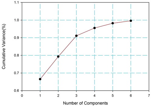
Figure 2. Principal components and their cumulative variance

In the empirical FAO-56 PM method, the central components influencing ETo calculations are temperature (maximum, minimum), wind speed, sunshine hours and humidity (maximum, minimum), and the latitude and altitude of the study area (Allen et al. 1998). The FAO-56 PM method has been widely studied and employed as a reliable means for prediction of ETo in several locations around the globe since 1998 (Bakhtiari et al. 2011, Kisi 2013; Subedi et al. 2013, Shiri et al. 2014, Caminha et al. 2017, Feng et al. 2017, Trigo et al. 2018).

The greatest shortcoming in the PM method is the need for complete climatic data in the ETo estimation (Droogers and Allen 2002). Machine learning methods have been adopted as important new methods in numerous fields in this epoch of fast innovation (Adamala et al. 2019). The prediction of ETo using artificial intelligence is no exception (Khoob 2008, Feng et al. 2017, Kovoor and Nandagiri 2018). Many studies reported in the literature have explored the success of neural network methods in the modelling of ETo and also effectively handled the limitations of traditional ETo estimation techniques (Partal 2009, Falamarzi et al. 2014, Trigo et al. 2018).

The variation in ETo directly influences the crop water requirements and irrigation schedule. However, ETo is very difficult to estimate accurately as the sensitivity of ETo depends upon various climatic factors and geographical factors. It is necessary to evaluate the impacts of such parameters on the sensitivity of ETo. This study provides a way to identify a reduced feature set with significant meteorological parameters needed for ETo prediction. There is no study in the literature on the application of a deep learning neural network (DLNN) with a reduced-feature data model to evaluate ETo. A further objective of this study is to evaluate the ability of the DLNN to estimate ETo for the data model obtained from the Veeranam tank with a reduced-feature dataset.

The paper is structured as follows: Section 2 discusses studies in the literature which have used machine learning as a modelling method for ETo prediction. Section 3 addresses the problem approach and Section 4 explains the theoretical approaches used in this work. In Section 5, the data model used is explored in detail. The experimental information for the artificial neural network (ANN) modelling is discussed in Section 6. Section 7 describes the modelling results, and the work is concluded in the final section.

2 Related work

Machine learning approaches seem widespread in recent years and are consistent in terms of their ETo predictions (Partal 2009, Kumar et al. 2011, Kisi 2011, Cobaner 2013, Falamarzi et al. 2014, Caminha et al. 2017, Feng et al. 2017, Manikumari et al. 2017, Valipour and Sefidkouhi 2018, Kovoor and Nandagiri 2018, Tikhamarine et al. 2019, Keshtegar et al. 2019).

ANNs were expansively explored in evapotranspiration modelling, because of their ability to obtain and project the multifaceted input and output relations without requiring an in-depth understanding of the underlying process Kisi and Yildirim 2005; Kim and Kim 2008; Shamshirband et al. 2016). Several studies have investigated the competence of neural network techniques such as generalized regression neural networks (Feng et al. 2017), wavelet neural networks (Kisi 2013) back propagation algorithm (Caminha et al. 2017, Kovoor and Nandagiri 2018), and conjugate gradient descent methods, which have proven to be efficient in ETo modelling. Many researchers have also investigated and employed radial basis function neural networks (RBFNNs) to evaluate ETo. Their results clearly demonstrated the ability of the RBFNN method, compared to other ANN methods, in calculating ETo (Trajkovic 2009, Ladlani et al. 2012, Petković et al. 2016, Sanikhani et al. 2019, Naidu and Majhi 2019, Hashemi and Sepaskhah 2020). In the context of time series studies, the convolutional neural network (CNN) is a deep learning model that has attracted great attention in recent years in modelling of ETo (Saggi and Jain 2019, Ferreira and da Cunha 2020). In many other applications, such as image recognition and other digital technology, CNN typically outperformed conventional machine learning models (Ji et al. 2018). However, CNN deep learning models with powerful capabilities are not very well studied in hydrological sciences (Keshtegar et al. 2019, Tikhamarine et al. 2019).

Reduction of features is a machine learning technique that targets a minimum set of attributes to find a resulting distribution that is as similar to the initial distribution as possible. ETo estimation involves several meteorological parameters which makes it complicated, so adopting feature reduction in this case would be beneficial. A few studies have attempted to obtain a reduced feature set for the estimation of evapotranspiration, using feature reduction techniques such as correlation analysis, gain ratio and Gini coefficient (Caminha et al. 2017). So far, to our knowledge, no recent study has examined the use of the DLNN with a reduced-feature data model to estimate ETo. Thus, in this study DLNN was used as a modelling approach in ETo forecasting with a reduced-feature data model. Data gathered in the period 1995–2016 from Veeranam water tank, located in Tamil Nadu, India, was used for the study. The most important contributions of this study are as follows:

• To analyse the significance of climatic factors for ETo using principal component analysis (PCA);

• To obtain a reduced-feature data model with only the major significant factors, as ETo estimation is presently difficult to achieve due to too many input parameters;

• To identify a DLNN as a prompt tool for ETo prediction that adapts best in the semi-arid region around Veeranam tank, Tamil Nadu, India; and

• To identify the direct influence of variation in ETo on the crop water requirements and irrigation schedule in the study area.

3 Study area

Veeranam tank system, situated 235 km south of Chennai in India, is the leading tank irrigation system with regard to the irrigation zone. In this study, the command region of Veeranam tank was used for the investigation. It receives water from the Lower Coleroon anicut system through a feeder canal and a small amount of surplus from other small tanks upstream of it, in addition to rainfall intercepted by its catchment. Veeranam tank is the largest wetland ecosystem in Tamil Nadu and is a migration point in the winter (October–March) for several rare species of waterfowl. In this work, climatic data were collected from the Indian Meteorological Observatory, Annamalai Nagar (11°25ʹN, 79°44ʹE).The climatic data include temperature (maximum, minimum), relative humidity (maximum, minimum), windspeed and sunshine hours on daily basis. Figure 1 depicts the problem methodology. The following steps are involved in the problem design:

Step 1. Perform data collection and data cleaning such as removing missing values.

Step 2. Estimate the ETo value using the FAO-56 PM method.

Step 3. Apply PCA on the Veeranam tank data, to obtain a reduced-feature data model.

Step 4. For the reduced-feature data model, develop the following prediction methods for training and test datasets:

• develop the RBFNN model, and

• develop the CNN deep learning model.

Step 5. Compare the predicted results of the training and test datasets with actual results obtained by the FAO-56 PM method.

Step 6. Compute and compare the various prediction measures and receiver operating characteristic (ROC) curves for the reduced-feature model using training and test datasets.

Data collected for this research between 1995 and 2016 are pre-processed for experimentation. Different climate parameters required for the FAO-56 PM method are selected in particular, while pre-processing the data and experimental work are then carried out with FAO-56 PM (Zotarelli et al. 2010). Then, neural network modelling is applied through implementation of DLNN and RBFNN. The performance measures calculated to find the optimal prediction method are presented in the Appendix.

4 Theoretical background

The theoretical approaches of neural network methods such as DLNN and RBFNN employed for modelling are discussed in this section.

4.1 FAO-56 PM method

A data model for Veeranam tank was created for the period 1995–2016. Throughout this time, this tank was successfully used for irrigation. Table 1 provides a comprehensive description of the data used. Table 2 displays the statistical characteristics of the model. The data gathered consist of highest and lowest temperature, maximum and minimum relative humidity, wind speed and sunshine hours. In order to delete outlier values (i.e. the data that deviate from the standard range of the normal data because of other physical factors), data pre-processing was performed. The FAO-56 PM equation is calculated daily to find ETo, as follows:

(1) $\mathrm{E}{\mathrm{T}}_{\mathrm{o}}=\frac{0.408\mathrm{\Delta }\left(R_n-\mathrm{S}\mathrm{H}\right)+\gamma \frac{\mathrm{C}\mathrm{a}}{T_{\mathrm{a}\mathrm{v}\mathrm{g}}+273}{U}_2\left(e_{\mathrm{s}}-e_{\mathrm{a}}\right)}{\mathrm{\Delta }+\gamma \left(1+\mathrm{C}\mathrm{d}\ast U_2\right)}$(1)

Table 1. Model scenario. See Table 2 for attributes

Properties	Description
Model	Data model
Period	1995–2016 (22 years)
Number of samples	8036 (1148 weeks)
Total number of attributes	6 + 1 (predicted label – ETo)
Attribute list	RHMX, RHMN, WS, TMAX, TMIN, SSH, ETo

Table 2. Statistical description of data model employed

Attribute	Description	Data type	Min	Max	Mean
RHMX (%)	Maximum relative humidity	Real	70	100	81.589
RHMN (%)	Minimum relative humidity	Real	33	100	59.267
WS (m s^−1)	Wind speed	Real	0.5	12.9	5.895
TMAX (°C)	Maximum temperature	Real	23	41.4	34.395
TMIN (°C)	Minimum temperature	Real	16	28.5	23.729
SSH (h)	Sunshine hours	Real	0	10.5	7.272
ETo (mm)	Reference evapotranspiration	Real	4.996	1.3472	3.890

where ETo is the reference evapotranspiration (mmd⁻¹); Δ is the saturation vapour pressure (kPa °C⁻¹); R_n is net solar radiation (MJm⁻²d⁻¹); SH is the soil heat flux (MJ m⁻² d⁻¹); γ is a psychometric constant (kPa°C⁻¹); Ca and Cd are constants, which vary according to the time step; e_s is the daily or hourly saturation vapour pressure (kPa); e_a is the daily or hourly mean actual vapour pressure (kPa); T_avg is the daily mean temperature (°C); U₂ denotes the wind speed (m s⁻¹); and e denotes the vapour pressure (kPa).

4.2 Principal component analysis

The PCA approach is used to reduce the input dimensions (climatic parameters) when these are large and the components are strongly correlated. In PCA, smaller artificial variables are calculated that represent the variance of the set of variables observed. The measured artificial variables are known as the principal components (PCs). PCA orthogonalizes the variables; then, the major variant components are selected and lesser ones are omitted from the data model. The PCA approach used is as follows (Ringnér 2008):

• For each data dimension of the data model used, subtract the mean.

• Figure out how far the dimensions vary from the mean to find the covariance matrix.

• Calculate the eigenvectors and eigenvalues of the covariance matrix.

• Based on the eigenvectors and eigenvalues, select the components to form a reduced feature vector.

• Generate the new data model by using the transpose vector feature and original data model.

4.3 Radial basis function neural networks

RBFNNs have a strong mathematical foundation and are among the more popular neural networks, with diverse applications in various fields. For the approximation of non-linear functions, RBFNNs provide a technique to map multidimensional spaces and are potentially faster than other ANNs in neural learning. The multi-layered RBFNN has an input layer, a hidden layer and a linear output layer. The hidden layer is fitted with a non-linear activation function (Trajkovic 2009, Ladlani et al. 2012, Petković et al. 2016, Naidu and Majhi 2019, Sanikhani et al. 2019, Hashemi and Sepaskhah 2020). The number of radial basis functions (RBFs) defining the activation functions of the hidden units is fixed. The Gaussian function is the most widely used RBF. The end result of the RBFNN may be given as:

(2) $y\left(x+d\right)={\sum }_{k=0}^n{W}_{ik}{\mathrm{\varnothing }}_i$(2)

where the weights between the neuron of the input layer i and the hidden layer k are as denoted W_ik, and y(x + d) is the predicted result in time x with delay d.

(3) ${\mathrm{\varnothing }}_i=\mathrm{e}\mathrm{x}\mathrm{p}[-{\left|x\left(t\right)-Ci\right|}^2/2{\sigma }^2$(3)

where i varies from 1 to n;AAAAis the applied Gaussian function on input x(t); and ci is the centre of the ith hidden layer neuron. Euclidean distance is obtained asBBBin Equation (3)(3) ${\mathrm{\varnothing }}_i=\mathrm{e}\mathrm{x}\mathrm{p}[-{\left|x\left(t\right)-Ci\right|}^2/2{\sigma }^2$(3) .

4.4 Deep learning neural network

The DLNN, employing a CNN developed with a specific set of components, is used in this analysis (Krizhevsky 2012, Jia et al. 2014). The CNN architecture is multi-layered, consisting of a convolution layer, a pooling layer, a dropout layer and a fully connected layer. The ETo prediction model is a time series one-dimensional (1D) data model. Here, the CNN takes the time series data in 1D form wherein the data are arranged in the order of sequential time instants. The convolutional layers of the CNN learn fast; the drop-out layer can slow the learning process and hopefully lead to a better final model. The pooling layer reduces the learning characteristics, consolidating them into only the most important components. With the dropout layer, the accuracy will gradually increase and loss will gradually decrease. The learned features after the dropout layer are flattened to a long vector after the convolution and pooling and go through a fully connected layer before the prediction layer. Rectifier linear units are most commonly used as an activation function in the convolutional layer. The activation function used in the output layer is maxout. The maxout activation used (Equations 4(4) $\mathrm{m}\mathrm{a}\mathrm{x}\mathrm{o}\mathrm{u}{\mathrm{t}}_i\left(x\right)=\mathrm{m}\mathrm{a}\mathrm{x}\left(z_{ij}\right)j\in \left[1,k\right]$(4) and 5(5) $z_{ij}\left(x\right)=x^T{W}_{ij}+b_{ik}$(5) ) does not have a zero gradient in deep networks.

(4) $\mathrm{m}\mathrm{a}\mathrm{x}\mathrm{o}\mathrm{u}{\mathrm{t}}_i\left(x\right)=\mathrm{m}\mathrm{a}\mathrm{x}\left(z_{ij}\right)j\in \left[1,k\right]$(4)

(5) $z_{ij}\left(x\right)=x^T{W}_{ij}+b_{ik}$(5)

where the network parameters W_ij and b_ij are the weight and the bias, respectively (Keshtegar et al. 2019, Tikhamarine et al. 2019).

5 Data model

The comprehensive and statistical details of the data model obtained in this study are shown in Tables 1 and Tables 2, respectively. Estimation of ETo is very difficult to achieve, as the sensitivity of ETo depends upon various climatic and geographical factors. It is necessary to evaluate the impacts of such parameters on the sensitivity of ETo. This section provides a method to reduce the size of the data model by choosing the significant meteorological parameters needed for ETo prediction.

5.1 Feature reduction

Six principal components (PC1–PC6) were obtained for the Veeranam tank data model using a PCA with six attributes (Fig. 2). To choose the significant PCs, the constraint of variance ≤0.95 is adopted. Thus, the number of PCs chosen for the data model is reduced from six to three, with three components (PC1, PC2 and PC3) each having a variance of less than 0.95 being obtained. For PC4–PC6, the variance is greater than the chosen constraint of 0.95, so those components are omitted.

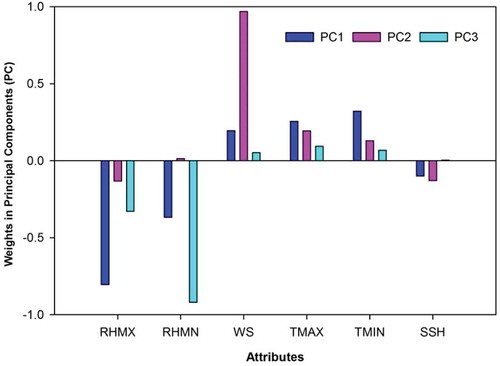
The weights of attributes of each chosen PC (PC1–PC3) are obtained; these are presented in Table 3 and Fig. 3. The values plotted in Fig. 3 show that the parameters TMAX, TMIN and WS alone have positive weight values for all three PCs, whereas the other parameters have negative weight values. Among the attributes, it is noted that TMAX, TMIN and WS have higher weight values (0.322, 0.256 and 0.195, respectively) for PC1; similar cases are noted for PC2 and PC3 (Table 3). So, for further analysis in this study, a reduced-feature data model is developed with the three significant parameters identified (TMAX, TMIN and WS). A description of the reduced-feature data model is given in Table 4.

Table 3. Attribute weights on selected principal components (PC)

Attribute	PC1	PC2	PC3
RHMX	−0.804	−0.132	−0.328
RHMN	−0.369	0.013	−0.919
WS	0.195	0.969	0.052
TMAX	0.256	0.194	0.094
TMIN	0.322	0.13	0.068
SSH	−0.1	−0.13	0.003

Figure 3. Attribution of weights in principal components

6 Modelling of ETo

Modelling is the principal approach of neural networks due to their ability to train data instances. The estimation of ETo was done experimentally using the FAO-56 PM method. The ANN modelling is implemented using the Weka tool. To show the effectiveness of the DLNN method, it was compared to RBFNN as the baseline method. The reduced-feature dataset is randomly split into a training dataset and a test dataset for learning and prediction. The training dataset consists of 80% of the reduced-feature data and the test dataset comprises the remaining 20% of the data. Both ANN models were analysed using the training and test datasets.

6.1 Parameter optimization of RBFNN

The RBFNN makes use of the k-means clustering technique. The number of k-means clusters is a major parameter in the RBFNN. For the RBFNN model, it is necessary to find an optimum value for the cluster number. Mean squared error (MSE) values were calculated to determine the best value for a random cluster; these are presented in Table 5. The table shows the MSE value variance in different clusters with training and test collection. It may be seen that the error decreases as the cluster count value increases from 10 to 20, while the MSE value again increases when the cluster count exceeds 20 (Table 5). The minimum MSE value of the data model is 0.8 for training and 0.06 for testing, with a cluster number of 20, while for a cluster number of 30, the MSE increases to 0.11 for training and 0.8 for testing. Thus, the optimum cluster number chosen for the RBFNN is 20.

Table 4. Scenario of the reduced-features data model

Properties	Description
Number of samples	8036 (1148 weeks)
Total number of attributes	3 + 1 (predicted label – ETo)
Reduced attribute list	TMAX, TMIN, WS
Prediction attribute	ETo
Number of training samples	6429 samples (80% of actual samples)
Number of training samples	1607 samples (20% of actual samples)

Table 5. Parameter optimization of the radial basis function neural network (RBFNN) architecture. MSE: mean squared error. Best values are indicated in bold

Number of clusters	MSE for training	MSE for testing
10	0.15	0.10
20	0.8	0.06
30	0.11	0.08
40	0.17	0.11
50	0.20	0.15

6.2 Parameter optimization of DLNN

This section explores the number of fully connected and convolutional layers, the optimal quantity of neurons for the fully connected layer, and other parameters needed for the CNN. The counts of convolutional and fully connected layers are the dominant parameters that control the performance of the CNN model. The number of convolutional layers plays a major role in reducing the data model variation and correlation. The fully connected layers gather the knowledge learned in the convolutional layers for discrimination of class. In this work, the CNN architecture was chosen by trial and error. Table 6 illustrates the MSE obtained by randomly varying the number of convolutional and fully connected layers for the training and testing datasets. Initially, to choose the number of convolution and fully connected layers, four different architecture combinations are considered. These combinations are obtained by randomly varying the number of convolution layers and fully connected layers, as shown in Table 6. The optimum architecture among these four is identified by calculating the MSE obtained for ETo prediction with default values for other CNN parameters available in the Weka tool. First, the CNN architecture is trained using the training data model; the prediction results obtained for the training data model are compared with the FAO-56 PM ETo values to find the MSE for the training data model. Table 6 reveals that the optimal number for the reduced-feature model is two convolution layers and one fully connected layer.

Table 6. Variation of mean squared error (MSE) with the number of convolution layers (conv) and fully connected (full) layers of the convolutional neural network (CNN). Bold formatting indicates the optimum number of layers

Number of layers	MSE for training	MSE for testing
1 conv, 1 full	0.25	0.25
1 conv, 2 full	0.22	0.23
2 conv, 1 full	0.19	0.22
2 conv, 2 full	0.36	0.32

The next major hyper-parameter in the CNN architecture is the number of neurons in the fully connected layer. To identify the optimum number of neurons for the one-layer fully connected architecture that was chosen, the number of neurons is varied randomly, as shown in Table 7. The table shows that as the number of neurons increases up to 30 for the training phase of the model, the MSE steadily decreases, after which a gradual rise in MSE is observed. The case for the testing dataset is similar. Thus, the optimum number of neurons in the fully connected layer was identified as 30. The other parameters in the CNN architecture use the default value available in the Weka tool, as shown in Table 8.

Table 7. Variation of the mean squared error (MSE) with the number of neurons in the fully connected layer of the convolutional neural network (CNN). Bold formatting indicates the optimum number of neurons

Number of neurons	MSE for training	MSE for testing
20	0.21	0.26
30	0.24	0.22
40	0.33	0.21
50	0.35	0.22
60	0.35	0.26

7 Results and discussion

The results calculated using the PM equation were modelled for prediction of ETo. The performance was measured in terms of mean absolute error (MAE), root mean square error (RMSE) and the regression coefficient (R²), the formulae for which are given in the Appendix.

Table 9 shows the results obtained from the DLNN and RBFNN methods. Among the ANN methods, it was noted that for the training and test datasets used, the DLNN model performed better than the RBFNN. With the training data, the RMSE is minimum for the DLNN (0.17), smaller by 0.07 than that of the RBFNN model. The MAE for the DLNN model is smaller by 0.06 than that of the RBFNN in training. With the testing dataset, the RMSE (of 0.21) is the minimum for the DLNN, 0.10 smaller than for the RBFNN model. The value of MAE for the DLNN model on the testing dataset is smaller by 0.09 than for the RBFNN model. The DLNN model performance was similar for the training and test datasets. Among the predictions made for the training and testing datasets, the DLNN performs better than the RBFNN. Both models performed better for the training dataset than for the testing dataset. This indicates that more fine tuning is needed to identify the optimum parameters for the neural network models used.

Table 8. Parameter values of the convolutional neural network (CNN) used in this study

Parameter	Value
Number of filters in convolutional layer	42
Kernel size	3
Dropout rate	0.1
Learning rate	0.001
Batch size	512
Learning model	Adam
Number of epochs	100

Table 9. Performance metrics for the artificial neural network (ANN) methods used in this study. DLNN: deep learning neural network; MAE: mean absolute error; RBFNN: radial basis function neural network; RMSE: root mean square error

Data model	Method	MAE		RMSE
Training	RBFNN	0.18	0.24
	DLNN	0.12	0.17
Testing	RBFNN	0.27	0.31
	DLNN	0.16	0.21

The time needed for the DLNN and RBFNN evaluation models in the Weka tool for the training and testing model evaluations was compared (Table 10). The PC configuration used was Windows 8, Intel Core Processor i7-2600 and 4 GB RAM quad-core CPU. The RBFNN predictions for the training and test datasets were performed in less time than those of the DLNN. This is because of the number of hidden layers and the huge number of iterations in the DLNN, although the DLNN is a suitable option in terms of prediction efficiency.

Table 10. Time taken to build the artificial neural network (ANN) methods. DLNN: deep learning neural network; RBFNN: radial basis function neural network

Data model	Method	Time taken (ms)
Training	RBFNN	1.05
	DLNN	3.43
Testing	RBFNN	0.04
	DLNN	2.9

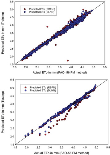
Figure 4 displays the scatterplots of the RBFNN and DLNN model results for the training and test datasets compared with the FAO-56 PM-calculated ETo. It is evident that the DLNN model estimates in the training and test phases are less dispersed than those of the RBFNN model (Fig. 4(a,b)). The comparison shows the RBFNN model gave more dispersed values, particularly for the test dataset. For the training and testing data, the DLNN model predicts ETo more effectively than the RBFNN does. Table 11 shows a comparison of the models in terms of the regression coefficient (R²), where the values for the DLNN model are 0.99 and 0.97 for the training and test datasets, respectively, which shows it is superior to the RBFNN model.

Table 11. Comparison of the artificial neural network (ANN) methods by regression coefficient, R². DLNN: deep learning neural network; RBFNN: radial basis function neural network

Data model	Method	R^2
Training	RBFNN	0.952
	DLNN	0.991
Testing	RBFNN	0.862
	DLNN	0.979

Figure 4. Scatterplots of DLNN and RBFN models for (a) the training dataset and (b) the testing dataset

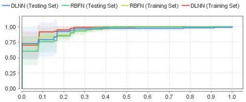
7.1 Visualizing the ROC curves

ROC curves provide the means to achieve accuracy of the predictions. The ROC curve plots the sensitivity against [1 – (false positive rate)] for successive cut-offs for the probability of an outcome. Each point on the ROC curve corresponds to a specific threshold, although the value of thresholds is not evident from the graph. The best prediction method is the one closest to the top left-hand corner of the ROC curve. Figure 5 shows the ROC curves of the DLNN and RBFNN models for training and testing data. It can be seen from Fig. 5 that the DLNN curve reaches the top left corner before the RBFNN curve. Thus, the performance of the DLNN method was superior to that of the RBFNN for ETo prediction.

Figure 5. Receiver operating characteristic (ROC) curve of the DLNN and RBFN models (training and testing)

8 Conclusion

This work explores how ETo is predicted by using a deep learning modelling approach on a reduced-feature data model. The findings are extremely promising. The DLNN has been explored extensively in several fields of science, but not yet in the prediction of ETo. This paper discussed the DLNN’s ability to predict ETo compared to the FAO-56 PM equation and a RBFNN model. The effectiveness of the DLNN model in the study area is also confirmed by the results in terms of regression coefficients. The possible cause of maximum correlation may be due to the number of neurons chosen in the DLNN architecture. The time taken by the DLNN for learning is greater than that of the RBFNN, which is due to the hidden neurons that are repeatedly tuned. The DLNN model was more reliable and accurate than the RBFNN in terms of prediction performance.

The RBFNN performs better than the DLNN when the R² values are compared (0.991 vs. 0.979 for the training and test data). Not surprisingly, the performance of the training data model is better than the output of the test data model. The lower RMSE and MSE on the training data model than the test data model also indicate that the DLNN architecture needs to pick even stronger hyper-parameters (Tables 6–Tables 8). The interactions between climate parameters used are more complex in the DLNN in this high-dimensional dataset, but the reduction in model features provides a positive effect in DLNN operation. This is evident from the prediction error, which represents a generalization of the DLNN architecture. It is also noted that the RBFNN models did not show impressive results in comparison with the DLNN when used in ETo prediction. This is because predictability depends primarily on the width of the hidden layer of the radial foundation in the RBFNN. Furthermore, the RBFNN endures the curse of dimensionality for high-dimensional problems like ETo prediction. The DLNN with TMAX, TMIN and wind speed as parameters proved to be a prompt tool for ETo prediction that is well adapted for the semi-arid region around Veeranam tank in Tamil Nadu, India. This research has shown that the DLNN model based on a reduced dataset of climatic features can be employed in irrigation scheduling and demand projections.

Disclosure statement

No potential conflict of interest was reported by the authors.

Appendix

The performance of the models studied was measured in terms of mean absolute error (MAE), root mean square error (RMSE) and the regression coefficient (R²). The formulae for these performance metrics are as follows:

(A1) $\mathrm{R}\mathrm{M}\mathrm{S}\mathrm{E}=\sqrt{\frac{{\sum }_{i=1}^N{\left(\mathrm{E}{\mathrm{T}}_{i,\mathrm{c}\mathrm{a}\mathrm{l}}-\mathrm{E}{\mathrm{T}}_{i,\mathrm{p}\mathrm{r}\mathrm{e}\mathrm{d}}\right)}^2}{N}}$(A1)

(A2) $\mathrm{M}\mathrm{A}\mathrm{E}=\frac{1}{N}{\sum }_{i=1}^N\left|\mathrm{E}{\mathrm{T}}_{i,\mathrm{c}\mathrm{a}\mathrm{l}}-\mathrm{E}{\mathrm{T}}_{i,\mathrm{p}\mathrm{r}\mathrm{e}\mathrm{d}}\right|\times 100$(A2)

(A3) $R^2=1-\frac{{\sum }_{i=1}^N{\left(\mathrm{E}{\mathrm{T}}_{i,\mathrm{c}\mathrm{a}\mathrm{l}}-\mathrm{E}{\mathrm{T}}_{i,\mathrm{p}\mathrm{r}\mathrm{e}\mathrm{d}}\right)}^2}{{\sum }_{i=1}^N{\left(\mathrm{E}{\mathrm{T}}_{i,\mathrm{c}\mathrm{a}\mathrm{l}}-\mathrm{m}\mathrm{e}\mathrm{a}\mathrm{n}\mathrm{E}{\mathrm{T}}_{\mathrm{p}\mathrm{r}\mathrm{e}\mathrm{d}}\right)}^2}$(A3)

where ET_i,cal is the ETo calculated by the FAO-56 PM method and ET_i,_pred is the ETo predicted by modelling; meanET_pred is the mean of predicted ETo; and N is the number of data.

References

- Adamala, S., et al., 2019. Generalized wavelet neural networks for evapotranspiration modeling in India. ISH Journal of Hydraulic Engineering, 25 (2), 119–131. doi:10.1080/09715010.2017.1327825
- Allen, R., et al., 1998. Crop evapotranspiration-guidelines for computing crop water requirements-FAO irrigation and drainage paper 56. Rome, Italy: Food and Agriculture Organization of the United Nations.
- Bakhtiari, B., et al., 2011. Evaluation of reference evapotranspiration models for a semiarid environment using lysimeter measurements. Journal of Agricultural Science and Technology, 13, 223–237.
- Caminha, H.D., et al., 2017. Estimating reference evapotranspiration using data mining prediction models and feature selection. International Conference on Enterprise Information Systems in ICEIS. 1, 272–279. doi:10.5220/0006327202720279
- Cobaner, M., 2013. Reference evapotranspiration based on Class A pan evaporation via wavelet regression technique. Irrigation Science, 31 (2), 119–134. doi:10.1007/s00271-011-0297-x
- Droogers, P. and Allen, R.G., 2002. Estimating reference evapotranspiration under inaccurate data conditions. Irrigation and Drainage Systems, 16 (1), 33–45. doi:10.1023/A:1015508322413
- Falamarzi, Y., et al., 2014. Estimating evapotranspiration from temperature and wind speed data using artificial and wavelet neural networks. Agricultural Water Management, 140, 26–36. doi:10.1016/j.agwat.2014.03.014
- Feng, Y., et al., 2017. Evaluation of random forests and generalized regression neural networks for daily reference evapotranspiration modelling. Agricultural Water Management, 193, 163–173. doi:10.1016/j.agwat.2017.08.003
- Ferreira, L.B. and da Cunha, F.F., 2020. New approach to estimate daily reference evapotranspiration based on hourly temperature and relative humidity using machine learning and deep learning. Agricultural Water Management, 234, 106113. doi:10.1016/j.agwat.2020.106113
- Hashemi, M. and Sepaskhah, A.R., 2020. Evaluation of artificial neural network and Penman–Monteith equation for the prediction of barley standard evapotranspiration in a semi-arid region. Theoretical and Applied Climatology, 139 (1), 275–285. doi:10.1007/s00704-019-02966-x
- Huntington, T.G. and Billmire, M., 2014. Trends in precipitation, runoff, and evapotranspiration for rivers draining to the Gulf of Maine in the United States. Journal of Hydrometeorology, 15 (2), 726–743. doi:10.1175/JHM-D-13-018.1
- Ji, S., et al., 2018. 3D convolutional neural networks for crop classification with multi-temporal remote sensing images. Remote Sensing. (Basel), 10 (2), 75. doi:10.3390/rs10010075
- Jia, Y., et al. 2014. Caffe: convolutional architecture for fast feature embedding. In: Proceedings of the 22nd ACM international conference on Multimedia, New York, USA. 675–678. November.
- Keshtegar, B., Kisi, O., and Zounemat-Kermani, M., 2019. Polynomial chaos expansion and response surface method for nonlinear modelling of reference evapotranspiration. Hydrological Sciences Journal, 64 (6), 720–730. doi:10.1080/02626667.2019.1601727
- Khoob, A.R., 2008. Artificial neural network estimation of reference evapotranspiration from pan evaporation in a semi-arid environment. Irrigation Sciences, 27 (1), 35–39. doi:10.1007/s00271-008-0119-y
- Kim, S. and Kim, H.S., 2008. Neural networks and genetic algorithm approach for nonlinear evaporation and evapotranspiration modelling. Journal of Hydrology, 351, 299–317. doi:10.1016/j.jhydrol.2007.12.014
- Kisi, Ö. and Yildirim, G., 2005. Forecasting of reference evapotranspiration by artificial neural networks. Journal of Irrigation and Drainage Engineering, 131 (4), 390–391. doi:10.1061/(ASCE)0733-9437
- Kisi, O., 2011. Modelling reference evapotranspiration using evolutionary neural networks. Journal of Irrigation and Drainage Engineering, 137 (10), 636–643. doi:10.1061/(ASCE)IR.1943-4774.0000333
- Kisi, O., 2013. Least squares support vector machine for modelling daily reference evapotranspiration. Irrigation Sciences, 31 (4), 611–619. doi:10.1061/(ASCE)0733-9437
- Kovoor, G.M. and Nandagiri, L., 2018. Sensitivity analysis of FAO-56 Penman–Monteith reference evapotranspiration estimates using Monte Carlo simulations. In: Dr. V.P. Singh, Prof. Dr. S. Yadav, Prof. Dr. R.N. Yadava, eds. Hydrological modelling. Singapore: Springer, 73–84.
- Kramer, R., et al., 2015. Evapotranspiration trends over the eastern United States during the 20th century. Hydrology, 2 (2), 93–111. doi:10.3390/hydrology2020093
- Krizhevsky, A., 2012. H., Hinton, GE: imagenet classification with deep CNN. Advances in Neural Information Processing Systems, 60 (6), 1097–1105.
- Kumar, M., Raghuwanshi, N.S., and Singh, R., 2011. Artificial neural networks approach in evapotranspiration modeling: a review. Irrigation Sciences, 29, 11–25. doi:10.1007/s00271-010-0230-8
- Ladlani, I., et al., 2012. Modeling daily reference evapotranspiration (ET 0) in the north of Algeria using generalized regression neural networks (GRNN) and radial basis function neural networks (RBFNN): a comparative study. Meteorology and Atmospheric Physics, 118 (3–4), 163–178. doi:10.1007/s00703-012-0205-9
- Manikumari, N., Murugappan, A., and Vinodhini, G., 2017. Time series forecasting of daily reference evapotranspiration by neural network ensemble learning for irrigation system. IOP Conference Series: Earth and Environmental Science, 80 (1), 012069. July. doi:10.1088/1755-1315/80/1/012069
- Naidu, D. and Majhi, B., 2019. Reference evapotranspiration modeling using radial basis function neural network in different agro-climatic zones of Chhattisgarh. Journal of Agrometeorology, 21 (3), 316–326.
- Partal, T., 2009. Modeling evapotranspiration using discrete wavelet transform and neural networks. Hydrological Processes: An International Journal, 23 (25), 3545–3555. doi:10.1002/hyp.7448
- Pereira, L.S., et al., 2015. Crop evapotranspiration estimation with FAO56: past and future. Agricultural Water Management, 147, 4–20. doi:10.1016/j.agwat.2014.07.031
- Petković, D., et al., 2016. Particle swarm optimization-based radial basis function network for estimation of reference evapotranspiration. Theoretical and Applied Climatology, 125 (3–4), 555–563. doi:10.1007/s00704-015-1522-y
- Ringnér, M., 2008. What is principal component analysis? Nature Biotechnology, 26 (3), 303–304. doi:10.1038/nbt0308-303
- Saggi, M.K. and Jain, S., 2019. Reference evapotranspiration estimation and modeling of the Punjab Northern India using deep learning. Computers and Electronics in Agriculture, 156, 387–398. doi:10.1016/j.compag.2018.11.031
- Sanikhani, H., et al., 2019. Temperature-based modeling of reference evapotranspiration using several artificial intelligence models: application of different modeling scenarios. Theoretical and Applied Climatology, 135 (1–2), 449–462. doi:10.1007/s00704-018-2390-z
- Shamshirband, S., et al., 2016. Estimation of reference evapotranspiration using neural networks and cuckoo search algorithm. Journal of Irrigation and Drainage Engineering, 142 (2), 04015044. doi:10.1061/(ASCE)IR.1943-4774.0000949
- Sharma, A.N. and Walter, M.T., 2014. Estimating long-term changes in actual evapotranspiration and water storage using a one-parameter model. Journal of Hydrology, 519 (B), 2312–2317. doi:10.1016/j.jhydrol.2014.10.014
- Shiri, J., et al., 2014. Comparison of heuristic and empirical approaches for estimating reference evapotranspiration from limited inputs in Iran. Computers and Electronics in Agriculture, 108, 230–241. doi:10.1016/j.compag.2014.08.007
- Subedi, A., Chávez, J.L., and Andales, A.A., 2013. Preliminary performance evaluation of the Penman–Monteith evapotranspiration equation in southeastern Colorado. Hydrology Days-Department of Civil and Environmental Engineering, 970, 84–90.
- Tabari, H. and HosseinzadehTalaee, P., 2013. Multilayer perceptron for reference evapotranspiration estimation in a semiarid region. Neural Computing and Applications, 23 (2), 341–348. doi:10.1007/s00521-012-0904-7
- Tikhamarine, Y., et al., 2019. Estimation of monthly reference evapotranspiration using novel hybrid machine learning approaches. Hydrological Sciences Journal, 64 (15), 15,1824–1842. doi:10.1080/02626667.2019.1678750
- Trajkovic, S., 2009. Comparison of radial basis function networks and empirical equations for converting from pan evaporation to reference evapotranspiration. Hydrological Processes: An International Journal, 23 (6), 874–880. doi:10.1002/hyp.7221
- Trigo, I.F., et al., 2018. Validation of reference evapotranspiration from Meteosat Second Generation (MSG) observations. Agricultural and Forest Meteorology, 259, 271–285. doi:10.1016/j.agrformet.2018.05.008
- Valipour, M. and Sefidkouhi, M.A.G., 2018. Temporal analysis of reference evapotranspiration to detect variation factors. International Journal of Global Warming, 14 (3), 385–401. doi:10.1504/IJGW.2018.090403
- Ventura, F., et al., 1999. An evaluation of common evapotranspiration equations. Irrigation Sciences, 18 (4), 163–170. doi:10.1007/s002710050058
- Zotarelli, L., et al., 2010. Step by step calculation of the Penman-Monteith evapotranspiration (FAO-56 method). Institute of Food and Agricultural Sciences. University of Florida.