Bayesian regional flood frequency analysis with GEV hierarchical models under spatial dependency structures

ABSTRACT

Bayesian hierarchical models have been increasingly used in regional flood frequency analysis due to their flexibility and ability to accommodate the spatial variability of flooding processes in distribution parameters. Hierarchical models based on the generalized extreme value (GEV) distribution are useful since they may combine scaling properties and distinct degrees of pooling in the shape parameter for improving quantile estimation. In this paper, we evaluate the benefits of combining a partial pooling approach and a formal description of the spatial latent processes that govern the distribution parameters. The application of the model in the Alto do São Francisco River catchment (Brazil) suggests that, despite obtaining similar estimates at gauged sites, prediction at ungauged counterparts may be substantially improved in densely gauged regions, in terms of accuracy and precision, by accounting for spatial dependency. In poorly gauged areas, however, no benefits in utilizing latent spatial processes for inference were verified.

KEYWORDS:

• regional flood frequency analysis
• Bayesian hierarchical models
• generalized extreme value (GEV) distribution
• partial pooling
• spatial dependency
• uncertainty

Editor A. Castellarin Associate editor I. Prosdocimi

1 Introduction

Reliable estimates of rare and extreme flood quantiles are required for designing hydraulic structures, for assessing potential flood hazards and establishing risk management strategies (Hall and Solomatine 2008), and for defining measures for increasing the resilience of flood-prone areas (McClymont et al. 2019). The complex and unpredictable nature of flooding events – along with their potential to produce economic losses and claim lives, and the well-known inference issues that stem from utilizing small samples, have demanded continuous efforts from the hydrologic community to develop inference frameworks that would improve accuracy and precision in the estimation of those quantiles associated with low exceedance probabilities. Common approaches for this purpose include the use of non-systematic data (e.g. Baker et al. 2003, Botero and Frances 2010, Fernandes et al. 2010), indirect estimation through rainfall–runoff modelling (e.g. Costa and Fernandes 2017), the extension of block-maxima time series (e.g. Khali and Adamowski 2014, Khalil et al. 2016, Jesus et al. 2020) and the peaks-over-threshold rationale (e.g. Bezac et al. 2014, Silva et al. 2014, 2016, 2017).

Most frequently, however, hydrologists and water resources engineers have resorted to the pooling of spatial information, via regional flood frequency analysis (RFFA), to increase estimation reliability. As a matter of fact, since the pioneering work of Dalrymple (1960) – which was built upon the scale invariance principle and the notion of index flood – and the formal and theoretical advances introduced by Hosking and Wallis (1997) under the L-moments framework, RFFA has become a very popular inference tool in hydrological sciences and practical engineering expedients (see e.g. O’Brien and Burn 2014, Basu and Srinivas 2016, Hailegeorgis and Alfredsen 2017, Ahani et al. 2020, and references therein). Index-flood-based methods for RFFA are easy to implement and directly allow the transfer of information for ungauged sites once a homogeneous region is defined. On the other hand, in practical terms, the underlying assumptions of index-flood formalism, particularly that of a common regional dimensionless distribution, are often not rigorously verified (Renard 2011). In addition, from an inference standpoint, a formal account of the uncertainties stemming from the index-flood modelling process and from prediction, which are paramount for flood risk management (Hall and Solomatine 2008, McMillan et al. 2017), is often unfeasible (the reader is kindly referred to Renard (2011) for a thorough discussion on this topic).

As an alternative to the index-flood approach, the use of Bayesian hierarchical models (BHMs) has gained appeal in regionalization studies in the past few years (Cooley et al. 2007, Kwon et al. 2008, Lima and Lall 2010, Renard 2011, Lima et al. 2016, Yan and Moradkhani 2016, Ahn et al. 2017, Wu et al. 2018, 2019, Ahn and Steinschneider 2019, Alexander et al. 2019). BHMs relate the spatial behaviour of a random variable to a latent spatial process through the parameters of a distributional model. By virtue of their design, BHMs may trivially bypass the limiting assumptions of the index-flood approach – mainly, that of scale invariance, since the spatial variation of the parameters may be readily accommodated at the modelling process level, possibly through the inclusion of covariates and spatial dependency structures. This would eliminate the requirement to define homogeneous regions, which is, more often than not, a subjective expedient (Renard 2011). Moreover, as with any Bayesian inference procedure, uncertainty estimation and propagation through all modelling steps is straightforward, which should be useful for flood risk assessment and for discriminating flood mitigation strategies on a probability-consequence basis.

A frequently used model for describing flood extremes in the context of BHM is the generalized extreme value (GEV) distribution, first introduced by Jenkinson (1955) (see e.g. Renard 2011, Dyrrdal et al. 2015, Lima et al. 2016, Thorarinsdottir et al. 2018). In fact, under somewhat general conditions (at least for the parent distributions commonly used in hydrology), the GEV model arises as the asymptotic form for the distribution of streamflow (annual) block maxima, which prompts its use in at-site and regional flood frequency analysis on the basis of theoretical arguments (Lima et al. 2016). Moreover, the GEV distribution encompasses distinct behaviours regarding the upper tail decay – exponential, subexponential and hyperexponential or upper-bounded, in agreement with the Fisher-Tippett-Gnedenko theorem – which makes it a flexible model for describing rare events in a broad spectrum of flooding regimes (Naghettini 2017).

Another useful feature of the GEV model in RFFA expedients is the potential scaling behaviour between the location and scale parameters and the drainage areas of catchments (Lima et al. 2016, Wu et al. 2018, 2019). This behaviour suggests that regression models with proper predictive skills may be readily obtained for such parameters by using the catchment size as the sole predictor. On the other hand, capturing the spatial variation of the GEV shape parameter by means of covariates remains a challenging task. In effect, the large-scale studies of Dyrrdal et al. (2015) and Thorarinsdottir et al. (2018), which encompassed maximum precipitation and floods, respectively, suggest that the probability of inclusion of covariates – as related to geographic location, precipitation regime and morphologic characteristics of the catchments – in the regression model for the GEV shape parameter is small, which, to some extent, highlights the practical difficulties in identifying appropriate regression models for such a quantity (Tyralis et al. 2019).

In view of the outlined problem, the GEV shape parameter is often assumed to be constant across the regions in which RFFA is performed (Cooley et al. 2007, Renard 2011, Yan and Moradkhani 2015), being possibly inferred under informative prior distributions (Martins and Stedinger 2000, Renard 2011) for limiting its range. This premise, however, may be too restrictive, especially in larger and more heterogeneous regions (Lima et al. 2016). In fact, as the geographic extent of the study region grows, the distinctions in climate, precipitation regime and terrain characteristics, which should control the flooding regimes (Tyralis et al. 2019), become more noticeable. As a result, the adoption of a common value for the shape parameter may entail some degree of bias in quantile estimates and underestimation of the associated uncertainty, in both gauged and ungauged sites.

Recent developments (e.g. Lima et al. 2016, Wu et al. 2018, 2019) have resorted to a partial pooling approach for modelling the GEV shape parameter at the regional scale. The reasoning behind this modelling strategy is “shrinking” the estimates of such a parameter towards a (common) regional mean value, while allowing some degree of deviation with respect to this value, which, in turn, should be large enough to reflect the non-homogeneous hydrological regimes across the region. This “shrinkage” would avoid having the shape parameter assume implausible values, particularly in those sites with very short samples – which is also the goal of the inference strategies discussed in the previous paragraph. Nonetheless, since no constraints are introduced in inference by means of prior uncertainty distributions, a more rigorous account on the regional variability of the GEV shape parameter is likely to be obtained under this framework (Lima et al. 2016), potentially increasing the reliability in the estimation of extreme quantiles.

Despite the promising results of the partial pooling approach of Lima et al. (2016), the GEV hierarchical model proposed by the authors relies on the assumptions of conditionally independent data and spatial independence of the model parameters, which, in practical terms, may be unrealistic (Renard 2011). In fact, several studies have suggested that both quantities may be highly correlated in space (see e.g. Bracken et al. 2016 and references therein). Particularly, the model parameters at each catchment may be thought of as arising from a spatially correlated random field that is driven by long-term climate characteristics (Cooley et al. 2007) and, as a result of this correlation, in cases where some of the spatial variation in the distribution parameters is accounted for by covariates (e.g. drainage area, latitude, longitude, elevation), the dependence structure manifests itself in the regression errors.

As demonstrated by Kjeldsen and Jones (2007, 2009) and Renard (2011), the spatial dependence in regression errors may impact the accuracy and precision of the estimates of the regional distribution parameters in the gauged sites utilized in RFFA. Considering spatial correlation may also reduce the variance of the predictive distribution at ungauged locations since, by conditioning the target site’s regression errors to those in nearby sites, one may benefit from the additional available information (i.e. the known regression errors at neighbour catchments) and, to some extent, constrain the inference during prediction (Renard 2011). As such, coupling a formal representation of the spatial dependence structure of the GEV parameters and the partial pooling framework for inferring the shape counterpart could improve the estimation of rare and extreme flood quantiles in RFFA expedients, albeit assessing whether and to what extent this assumption would hold calls for further investigation.

In view of the foregoing, this paper discusses an extension to the partial pooling model of Lima et al. (2016) that formally incorporates spatial dependence structures for the GEV parameters. As a working hypothesis, we assume that the spatial random fields for each of the GEV parameters are described by Gaussian multivariate distributions, for which the variance–covariance matrices are defined under concepts borrowed from geostatistics. Despite some simplifying modelling assumptions (discussed below), we expect to provide a comprehensive and robust assessment of the benefits and shortcomings of the inclusion of spatial dependence in partial pooling-based RFFA. The reminder of the paper is organized as follows. Section 2 presents the methodology, including a description of the study area and the utilized dataset, and the construction of the Bayesian hierarchical structure for estimating the GEV parameters under spatial dependency, with a focus on the modelling assumptions. Section 3 presents a full application of the proposed modelling strategy to a collection of sites in the Alto do São Francisco river catchment, in the Brazilian state of Minas Gerais, as well as a comparison to a spatially independent model. Finally, the conclusions and research developments are addressed in Section 4.

2 Methodology

2.1 Study area and dataset

We apply the proposed Bayesian hierarchical approach to a set of streamflow gauging stations in the Alto do São Francisco river catchment, which lies in the central region of the Brazilian state of Minas Gerais (Fig. 1). This catchment is located in a region with subtropical climate characteristics and strong seasonality and drains an area of approximately 90 000 km² (CPRM 2001). Mean annual rainfall amounts range from 1000 mm in the northern portion of the catchment to 1700 mm in the southern part, with approximately 55% of these volumes occurring in the months of November through January. Evaporative demands, in turn, amount to on average 1000 mm/year (ANA 2003).

Figure 1. The Alto do São Francisco River catchment with the drainage system and the stream gauging stations selected for this study (left) and location map (right)

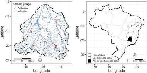
Mean daily streamflow information is available in 63 gauging stations in the study area (CPRM 2001). Data may accessed be through the Brazilian National Water Agency (ANA) digital platform (http://www.snirh.gov.br/hidroweb). To avoid physical inconsistencies in the regression models due to the distinct dependency structures across the river network, we have randomly selected a single site in the case of nested catchments. This reduced our calibration dataset to 31 gauging stations (see Fig. 1), whose ANA codes, drainage areas and sample sizes are presented in Table 1. It should be noted that the elimination process resulted in a more densely gauged region in the southern portion of the study area and relatively poorly gauged regions in the rest of the study area, as shown in Fig. 1 (the implications of this setup will be further discussed in Section 3).

Table 1. Streamflow gauging stations utilized for regional flood frequency analysis. N is the length of the maximum annual daily streamflow series

Code	Area (km^2)	N	Code	Area (km^2)	N	Code	Area (km^2)	N
40830000	84	13	40975000	964	18	40037000	765	25
40577000	244	21	40060001	559	49	40050000	5426	56
40530000	481	22	41340000	4874	42	40300001	1558	25
41050000	1207	31	40930000	876	25	40053000	304	30
40180000	144	11	40170000	1055	28	41300000	626	50
41250000	676	23	41380000	553	21	41780002	3996	23
40818000	273	20	40400000	1802	40	41890000	1435	22
41075001	4143	11	40770000	675	15	40067000	8987	10
40040000	259	31	40579995	579	46	40800001	5680	57
40056002	334	22	40330000	7378	47	40960000	1744	20
40573000	291	15	40710000	2760	25	41818000	16722	46
40790000	188	18	40032000	763	24

For the prediction step, four gauging stations, also shown in Table 1 and Fig. 1, were selected among those excluded from the training dataset. Two of the validation sites are located in the southern portion of the catchment and have a large number of close neighbours. The other two have a lower number of nearby sites, and these are relatively distant from the target locations. The main objective in selecting these sites for validation is to assess the performance of the spatially dependent model, hereafter termed M1, and of the spatially independent variant proposed by Lima et al. (2016), hereafter denoted M2, in distinct conditions of spatial hydrological information availability.

2.2 Bayesian GEV hierarchical model with spatial dependency structure

The GEV distribution is frequently used in statistical analysis of extremes and is a well-established model in flood frequency analysis (e.g. Sene et al. 2001, He et al. 2015). The cumulative distribution function of the GEV distribution, according to the parameterization adopted by Coles (2001), is given by

(1) $F\left(x\right)=\mathrm{e}\mathrm{x}\mathrm{p}\left\{-{\left[1+\xi \left(\frac{x-\mu }{\sigma }\right)\right]}^{-1/\xi }\right\}$(1)

in which $\mu$, $\sigma$ and $\xi$ are, respectively, location, scale and shape parameters. When $\xi <0$, the GEV model becomes the extreme value type II (EV2) distribution, with domain $\mu -\sigma /\xi <x<\mathrm{\infty }$. On the other hand, when $\xi >0$, the GEV model becomes the upper-bounded EV3 or Weibull distribution, with domain $x<\mu +\sigma /\xi$. The limiting case when $\xi =0$ corresponds to the EV1 or Gumbel distribution, with domain $-\mathrm{\infty }<x<\mathrm{\infty }$.

To derive the regional hierarchical model, we must first define the structure of the modelling layers and the mechanisms of interaction among them. Generally, the first layer is related to the probabilistic description of the data. As such, let us assume that, at a given site s (gauged or ungauged) and time t, the maximum annual streamflow, represented by $Y_{s,t}$, follows a GEV distribution with parameters that vary in space (but not in time). Formally,

(2) $Y\left(s,t\right)\sim \mathrm{G}\mathrm{E}\mathrm{V}\left[\mu \left(s\right),\sigma \left(s\right),\xi \left(s\right)\right]$(2)

To focus solely on the effects of spatial dependency structures assumed for the GEV parameters, we build our model under the assumption of conditional independence of data (i.e. the likelihood function arises from the product of the marginal distributions in each site, at each time step). This is, of course, a simplifying assumption that would “inflate” the actual information content of the pooled sample, potentially leading to underestimation of the variances of the inferred parameters and quantiles (Renard 2011). However, empirical evidence suggests that the correlation levels in the observations from our training dataset are not too high and, as a result, we believe that neither inference nor predictions should be strongly affected by this hypothesis.

The second modelling layer corresponds to a description of the spatial latent process, which accommodates the maximum annual floods’ spatial structure of variability in the GEV parameters. The process level is usually made up of the regression models and the regression errors. Here, two distinct approaches are utilized for estimating the GEV parameters through regression analysis. For the distribution’s location and scale parameters, we resort to the scaling theory (Gupta and Waymire 1990, Gupta et al. 1994, 2007, Gupta and Dawdy 1995, Morrison and Smith 2002, Northrop 2004, Lima and Lall 2010, Villarini et al. 2010, 2011, Ishak et al. 2011, Lima et al. 2016), thereby using the drainage area as a covariate in the regression model. As demonstrated by Lima et al. (2016), a log-linear relationship between the referred quantities is, frequently, a feasible functional form in this case. For the shape parameter, on the other hand, a partial pooling around a regional (unknown) mean value is adopted, and no covariates are included in the inference.

The regression errors, in turn, are intended to account for the variability left unexplained by the regression models of the GEV parameters. In the Bayesian hierarchical approach, such quantities are treated as latent variables that must be inferred along with other model parameters (Renard 2011). We assume, for simplicity, that the regression errors, for each of the GEV parameters, are realizations of independent Gaussian processes with variance–covariance matrices materialized by variograms. As a result, the spatial dependency structure is defined on the basis of the Euclidian distance between gauging stations.

Arguably, the Euclidian distance might not be the most appropriate descriptor of the spatial dependency structure of the GEV parameters in the context of maximum floods (Renard 2011, Thorarinsdottir et al. 2018). In fact, such a distance does not accommodate the river hierarchy when prescribing the intersite dependences and, as a result, does not take into account the nested nature of the stream network and the stronger dependence of connected basins during model calibration (Müller and Thompson 2015). However, due to the scaling behaviour of the GEV location and scale parameters, regression models with proper prediction skills are likely to be obtained by using the drainage areas as covariates (Lima et al. 2016), which would, at least to some extent, reduce the influence of the dependency structure in the estimation of such quantities (Kjeldsen and Jones 2009, Renard 2011). In addition, Ahn and Palmer (2016) and Tyralis et al. (2019) suggest that precipitation characteristics, which exhibit marked spatial patterns that stem from climate and terrain features and often present some degree of similarity in neighbouring catchments, are paramount for predicting the shape parameter of the GEV model that governs the frequencies of maximum floods.

In view of these arguments, we have resorted to geostatistics tools to estimate the regression errors’ covariances at the BHM process level, although we acknowledge that a more rigorous approach to deal with this issue appears to be necessary. Moreover, as previously stated, we have kept a single catchment among nested physiographic units for calibrating the regression models in order to avoid unsuitable representations of the spatial dependency structure along the river network that could stem from the correlations between the regression errors – such as having larger flood quantile estimates for the upstream gauge than those of the downstream gauge (Müller and Thompson 2015). This procedure, however, leads to larger variances of the posterior distributions for parameters and quantiles as it reduces the information content available for inference and fails to benefit from the higher degrees of dependence among gauges in nested catchments.

Following Yan and Moradkhani (2015), Bracken et al. (2016) and Ahn et al. (2017), we made use of exponential semivariograms to model the covariances across the spatial random fields. Hence, by taking $k\in \left\{\mu ,\sigma ,\xi \right\}$, one may define the covariance function as

(3) ${\mathbf{\Sigma }}_{\mathit{k}}=\left\{\begin{array}{c}{\delta }_k^2\cdot \mathrm{e}\mathrm{x}\mathrm{p}\left(-\frac{1}{{\varphi }_k}\parallel {\mathit{s}}_i-{\mathit{s}}_j\parallel \right),i\ne j\\ {\delta }_k^2+{\tau }_k^2,i=j\end{array}\right.$(3)

in which ${{\delta }_k}^2$ is the marginal variance of the regression errors for parameter k (or partial sill), ${\varphi }_k$ is the range, ${\tau }_k$ is the nugget and$\parallel {\mathit{s}}_{\mathit{i}}-{\mathit{s}}_{\mathit{j}}\parallel$is the matrix Euclidian distance between sites i and j.

From the previous assumptions, and assuming that no cross-correlation exists between regression errors from distinct GEV parameters, the process layer of the BHM may be formalized as follows:

$\mathrm{l}\mathrm{o}\mathrm{g}\left(\mu \left[{\tilde{s}}_i\right]\right)={\alpha }_0+{\alpha }_1\cdot \mathrm{l}\mathrm{o}\mathrm{g}\left(A\left[{\tilde{s}}_i\right]\right)+{\epsilon }_{\mu }\left({\tilde{s}}_i\right),\left({\epsilon }_{\mu }\left[{\tilde{s}}_1\right],\dots ,{\epsilon }_{\mu }\left[{\tilde{s}}_M\right]\right)\sim N\left(0,{\mathbf{\Sigma }}_{\mathit{\mu }}\right)$

$\mathrm{l}\mathrm{o}\mathrm{g}\left(\mu \left[{\tilde{s}}_i\right]\right)={\beta }_0+{\beta }_1\cdot \mathrm{l}\mathrm{o}\mathrm{g}\left(A\left[{\tilde{s}}_i\right]\right)+{\epsilon }_{\mu }\left({\tilde{s}}_i\right),\left({\epsilon }_{\mu }\left[{\tilde{s}}_1\right],\dots ,{\epsilon }_{\mu }\left[{\tilde{s}}_M\right]\right)\sim N\left(0,{\mathbf{\Sigma }}_{\mathit{\mu }}\right)$

(4) $\xi \left({\tilde{s}}_i\right)=\bar{\xi }+{\epsilon }_{\xi }\left({\tilde{s}}_i\right),\left({\epsilon }_{\xi }\left[{\tilde{s}}_1\right],\dots ,{\epsilon }_{\xi }\left[{\tilde{s}}_M\right]\right)\sim N\left(0,{\mathbf{\Sigma }}_{\mathit{\xi }}\right)$(4)

in which, following the notation in Renard (2011), ${\tilde{s}}_i,i=1,\dots ,M$ denotes the gauged sites from the calibration dataset, and ${\mathbf{\Sigma }}_{\mu }$, ${\mathbf{\Sigma }}_{\sigma }$ and ${\mathbf{\Sigma }}_{\xi }$ are the covariance matrix for each GEV parameter. Note that, according to our formalism, the deviations with respect to $\bar{\xi }$ are interpreted in a similar manner to the regression errors for the remaining GEV parameters.

The last modelling layer is that of the prior distributions for the parameters of both the regression models and the variograms, as well as for $\bar{\xi }$. Here, we considered weakly informative prior distributions (for a generic parameter $\vartheta$, $p\left(\vartheta \right)\propto 1$), mainly based on Bracken et al. (2016) and Lima et al. (2016). In the computational implementation, we set zero mean Gaussian distributions with standard deviations of 0.1, 1 and 10, for the sets of parameters (${\delta }_{\xi }^2,{\tau }_{\xi }^2$), (${\delta }_{\mu }^2,{\delta }_{\sigma }^2,{\tau }_{\mu }^2,{\tau }_{\sigma }^2$) and (${\alpha }_0,{\beta }_0$), respectively. For parameters $({\varphi }_{\mu },{\varphi }_{\sigma },{\varphi }_{\xi }$), normal distributions with mean and standard deviation equal to 50 for the parameters were elicited (Najafi and Moradkhani 2013, Yan and Moradkhani 2015). The remaining parameters were assigned uniform prior distributions, with range [−2, 2] for $\bar{\xi }$, and [0, 2] for${\alpha }_1$ and ${\beta }_1$.

2.3 Estimation at gauged sites

Suppose that in a given region, a set of gauged sites ${\tilde{s}}_i,i=1,\dots ,M$, each one containing a series of annual maximum streamflow $\tilde{y}\left({\tilde{s}}_i,t\right)$ with length $N_{{\tilde{s}}_i}$, is available for calibrating the BHM. Given the hierarchical structure discussed in the previous section, the joint posterior distribution of the model parameters, conditioned on the pooled sample $\tilde{\mathit{y}}$ and on covariates $\mathbf{x}$ (here, the drainage areas of the calibration sites), may be expressed as

(5) $\begin{array}{rl}& p(\mathit{\theta }|\tilde{\mathit{y}},\mathit{x})\propto \left[{\mathrm{\Pi }}_{{\tilde{s}}_i=1}^M{\mathrm{\Pi }}_{t=1}^{N{\tilde{s}}_i}f(y({\tilde{s}}_i,t)|\mu ({\tilde{s}}_i),\sigma ({\tilde{s}}_i),\xi ({\tilde{s}}_i))\right]\\ & \cdot \mathrm{M}\mathrm{V}\mathrm{N}\left(log(\mu (\tilde{\mathit{s}}))|{\alpha }_0+{\alpha }_1\cdot log(A(\tilde{\mathit{s}})),{\mathbf{\Sigma }}_{\mu }\right)\\ & \cdot \mathrm{M}\mathrm{V}\mathrm{N}\left(log(\sigma (\tilde{\mathit{s}}))|{\beta }_0+{\beta }_1\cdot log(A(\tilde{\mathit{s}})),{\mathbf{\Sigma }}_{\sigma }\right)\\ & \cdot \mathrm{M}\mathrm{V}\mathrm{N}\left(\xi (\tilde{\mathit{s}})|\bar{\xi },{\mathbf{\Sigma }}_{\mathit{\xi }}\right)\end{array}$(5)

in which vector $\mathit{\theta }$ includes the parameters of the variograms (Equation (3)(3) ${\mathbf{\Sigma }}_{\mathit{k}}=\left\{\begin{array}{c}{\delta }_k^2\cdot \mathrm{e}\mathrm{x}\mathrm{p}\left(-\frac{1}{{\varphi }_k}\parallel {\mathit{s}}_i-{\mathit{s}}_j\parallel \right),i\ne j\\ {\delta }_k^2+{\tau }_k^2,i=j\end{array}\right.$(3) ), the parameters of the regression models (Equation (4)(4) $\xi \left({\tilde{s}}_i\right)=\bar{\xi }+{\epsilon }_{\xi }\left({\tilde{s}}_i\right),\left({\epsilon }_{\xi }\left[{\tilde{s}}_1\right],\dots ,{\epsilon }_{\xi }\left[{\tilde{s}}_M\right]\right)\sim N\left(0,{\mathbf{\Sigma }}_{\mathit{\xi }}\right)$(4) ), and the regression errors for each of the GEV parameters. The term inside square brackets denotes the likelihood function, and those remaining on the right-hand side of the equation describe the process level of the BHM; of these, $\mathrm{M}\mathrm{V}\mathrm{N}\left(\mathbf{z}|\mathbf{m},\mathbf{\Sigma }\right)$ represents the multivariate normal distribution, with vector of means m and variance–covariance matrix $\mathbf{\Sigma }$, evaluated at generic points z.

To explore the posterior distribution in Equation (5)(5) $\begin{array}{rl}& p(\mathit{\theta }|\tilde{\mathit{y}},\mathit{x})\propto \left[{\mathrm{\Pi }}_{{\tilde{s}}_i=1}^M{\mathrm{\Pi }}_{t=1}^{N{\tilde{s}}_i}f(y({\tilde{s}}_i,t)|\mu ({\tilde{s}}_i),\sigma ({\tilde{s}}_i),\xi ({\tilde{s}}_i))\right]\\ & \cdot \mathrm{M}\mathrm{V}\mathrm{N}\left(log(\mu (\tilde{\mathit{s}}))|{\alpha }_0+{\alpha }_1\cdot log(A(\tilde{\mathit{s}})),{\mathbf{\Sigma }}_{\mu }\right)\\ & \cdot \mathrm{M}\mathrm{V}\mathrm{N}\left(log(\sigma (\tilde{\mathit{s}}))|{\beta }_0+{\beta }_1\cdot log(A(\tilde{\mathit{s}})),{\mathbf{\Sigma }}_{\sigma }\right)\\ & \cdot \mathrm{M}\mathrm{V}\mathrm{N}\left(\xi (\tilde{\mathit{s}})|\bar{\xi },{\mathbf{\Sigma }}_{\mathit{\xi }}\right)\end{array}$(5) , we utilize the No-U-Turn (NUTS) sampler, a variation of the Hamiltonian Monte Carlo (HMC) Markov chain Monte Carlo (MCMC) algorithm (Hoffman and Gelman 2014). The algorithm is implemented in the open-source Bayesian inference software Stan, accessed through the package RStan (Stan Development Team 2020) in the R environment, and is free for use (http://doi.org/10.5281/zenodo.4021683).

At the gauged sites $\tilde{s}$, the posterior distributions of the GEV parameters can be trivially approximated by the MCMC samples obtained from Equation (5)(5) $\begin{array}{rl}& p(\mathit{\theta }|\tilde{\mathit{y}},\mathit{x})\propto \left[{\mathrm{\Pi }}_{{\tilde{s}}_i=1}^M{\mathrm{\Pi }}_{t=1}^{N{\tilde{s}}_i}f(y({\tilde{s}}_i,t)|\mu ({\tilde{s}}_i),\sigma ({\tilde{s}}_i),\xi ({\tilde{s}}_i))\right]\\ & \cdot \mathrm{M}\mathrm{V}\mathrm{N}\left(log(\mu (\tilde{\mathit{s}}))|{\alpha }_0+{\alpha }_1\cdot log(A(\tilde{\mathit{s}})),{\mathbf{\Sigma }}_{\mu }\right)\\ & \cdot \mathrm{M}\mathrm{V}\mathrm{N}\left(log(\sigma (\tilde{\mathit{s}}))|{\beta }_0+{\beta }_1\cdot log(A(\tilde{\mathit{s}})),{\mathbf{\Sigma }}_{\sigma }\right)\\ & \cdot \mathrm{M}\mathrm{V}\mathrm{N}\left(\xi (\tilde{\mathit{s}})|\bar{\xi },{\mathbf{\Sigma }}_{\mathit{\xi }}\right)\end{array}$(5) . In formal terms, each MCMC replicate provides a realization for the parameters of the regression models and the corresponding regression errors, which are then combined to yield the estimates for the GEV parameters (Equation (4)(4) $\xi \left({\tilde{s}}_i\right)=\bar{\xi }+{\epsilon }_{\xi }\left({\tilde{s}}_i\right),\left({\epsilon }_{\xi }\left[{\tilde{s}}_1\right],\dots ,{\epsilon }_{\xi }\left[{\tilde{s}}_M\right]\right)\sim N\left(0,{\mathbf{\Sigma }}_{\mathit{\xi }}\right)$(4) ). Additionally, the posterior distribution of the T-year quantiles, which are often the main objective of RFFA, can be readily derived at sites $\tilde{s}$ by utilizing the parameter values calculated in the previous step and the GEV quantile function.

2.4 Prediction at ungauged sites

At a given ungauged site $\hat{s}$, one has available the parameters of regression models for the GEV parameters and those of the variograms, but not the corresponding regression errors. As a result, the latter’s distributions must be inferred from those derived for the regression errors at the gauged sites utilized for model calibration. Following Renard (2011) – and generically denoting the variograms’ parametric vectors as $\mathit{\nu }$, the distribution of the regression errors at site $\hat{s}$, conditioned to their counterparts in sites $\tilde{\mathit{s}}$ (and also to $\tilde{\mathit{y}}$, $\mathit{x}$, and $\mathit{\nu }$), may be expressed as follows (the full derivation is presented in Renard 2011):

(6) $p\left({\epsilon }_k\left[\hat{s}\right]|{\epsilon }_k\left[{\tilde{s}}_1\right],\dots ,{\epsilon }_k\left[{\tilde{s}}_M\right],{\mathit{\nu }}_k,\tilde{\mathit{y}},\mathit{x}\right)=N\left({\mu }_{k,\mathrm{c}\mathrm{o}\mathrm{n}\mathrm{d}\mathrm{i}\mathrm{t}\mathrm{i}\mathrm{o}\mathrm{n}\mathrm{a}\mathrm{l}},{\sigma }_{k,\mathrm{c}\mathrm{o}\mathrm{n}\mathrm{d}\mathrm{i}\mathrm{t}\mathrm{i}\mathrm{o}\mathrm{n}\mathrm{a}\mathrm{l}}^2\right)$(6)

in which $k\in \left\{\mu ,\sigma ,\mathit{\xi }\right\}$. The distribution in Equation (6)(6) $p\left({\epsilon }_k\left[\hat{s}\right]|{\epsilon }_k\left[{\tilde{s}}_1\right],\dots ,{\epsilon }_k\left[{\tilde{s}}_M\right],{\mathit{\nu }}_k,\tilde{\mathit{y}},\mathit{x}\right)=N\left({\mu }_{k,\mathrm{c}\mathrm{o}\mathrm{n}\mathrm{d}\mathrm{i}\mathrm{t}\mathrm{i}\mathrm{o}\mathrm{n}\mathrm{a}\mathrm{l}},{\sigma }_{k,\mathrm{c}\mathrm{o}\mathrm{n}\mathrm{d}\mathrm{i}\mathrm{t}\mathrm{i}\mathrm{o}\mathrm{n}\mathrm{a}\mathrm{l}}^2\right)$(6) is a Gaussian univariate model, from which one may randomly simulate the regression errors. The inferred regression models, along with the simulated regression errors, are then used to estimate the GEV parameters at site $\hat{s}$, and hence to construct the quantile curves and estimate the associated predictive uncertainty.

To estimate the values of ${\mu }_{k,\mathrm{c}\mathrm{o}\mathrm{n}\mathrm{d}\mathrm{i}\mathrm{t}\mathrm{i}\mathrm{o}\mathrm{n}\mathrm{a}\mathrm{l}}$ and ${\sigma }_{k,\mathrm{c}\mathrm{o}\mathrm{n}\mathrm{d}\mathrm{i}\mathrm{t}\mathrm{i}\mathrm{o}\mathrm{n}\mathrm{a}\mathrm{l}}^2$, let us define, for each parameter k, the $M\times M$ variance–covariance matrix of (known) regression errors, ${\mathbf{\Omega }}_k$, estimated from the calibration dataset, a $1\times M$ vector ${\mathbf{\Lambda }}_k$ containing the covariances between the regression error in the target site $\hat{s}$ and those inferred in sites $\tilde{s}$, and the marginal variance of the regression errors ${\sigma }_k^2$ (the notation is similar to that in Renard 2011). Also, let us aggregate these components in a new variance–covariance matrix ${\mathbf{\Gamma }}_k$, which is intended to account for the contribution of each site $\tilde{s}$ to the regression errors in the site $\hat{s}$. In formal terms (Renard 2011):

(7) ${\mathbf{\Gamma }}_k=\left(\begin{array}{cc}{\sigma }_k^2& {\mathbf{\Lambda }}_k\\ {\mathbf{\Lambda }}_k^t& {\mathbf{\Omega }}_k\end{array}\right)$(7)

The parameters for the Gaussian distribution in Equation (6)(6) $p\left({\epsilon }_k\left[\hat{s}\right]|{\epsilon }_k\left[{\tilde{s}}_1\right],\dots ,{\epsilon }_k\left[{\tilde{s}}_M\right],{\mathit{\nu }}_k,\tilde{\mathit{y}},\mathit{x}\right)=N\left({\mu }_{k,\mathrm{c}\mathrm{o}\mathrm{n}\mathrm{d}\mathrm{i}\mathrm{t}\mathrm{i}\mathrm{o}\mathrm{n}\mathrm{a}\mathrm{l}},{\sigma }_{k,\mathrm{c}\mathrm{o}\mathrm{n}\mathrm{d}\mathrm{i}\mathrm{t}\mathrm{i}\mathrm{o}\mathrm{n}\mathrm{a}\mathrm{l}}^2\right)$(6) may be then computed by (Renard 2011):

(8) ${\mu }_{k,\mathrm{c}\mathrm{o}\mathrm{n}\mathrm{d}\mathrm{i}\mathrm{t}\mathrm{i}\mathrm{o}\mathrm{n}\mathrm{a}\mathrm{l}}={\mathbf{\Lambda }}_k{\mathbf{\Omega }}_k^{-1}{\left({\epsilon }_k\left[{\tilde{s}}_1\right],\dots ,{\epsilon }_k\left[{\tilde{s}}_M\right]\right)}^t$(8)

(9) ${\sigma }_{k,\mathrm{c}\mathrm{o}\mathrm{n}\mathrm{d}\mathrm{i}\mathrm{t}\mathrm{i}\mathrm{o}\mathrm{n}\mathrm{a}\mathrm{l}}^2={\sigma }_k^2-{\mathbf{\Lambda }}_k{\mathbf{\Omega }}_k^{-1}{\mathbf{\Lambda }}_k^t$(9)

Equation (8)(8) ${\mu }_{k,\mathrm{c}\mathrm{o}\mathrm{n}\mathrm{d}\mathrm{i}\mathrm{t}\mathrm{i}\mathrm{o}\mathrm{n}\mathrm{a}\mathrm{l}}={\mathbf{\Lambda }}_k{\mathbf{\Omega }}_k^{-1}{\left({\epsilon }_k\left[{\tilde{s}}_1\right],\dots ,{\epsilon }_k\left[{\tilde{s}}_M\right]\right)}^t$(8) shows that the expected value of the regression error at the ungauged site amounts to a weighted average from those estimated during model calibration, with more weight provided to the closest catchments. Moreover, one may note from Equation (9)(9) ${\sigma }_{k,\mathrm{c}\mathrm{o}\mathrm{n}\mathrm{d}\mathrm{i}\mathrm{t}\mathrm{i}\mathrm{o}\mathrm{n}\mathrm{a}\mathrm{l}}^2={\sigma }_k^2-{\mathbf{\Lambda }}_k{\mathbf{\Omega }}_k^{-1}{\mathbf{\Lambda }}_k^t$(9) that by conditioning the inference of the regression errors at the target site to those already inferred from the calibration dataset, a reduction in the predictive variances of the parameters and, accordingly, those of the quantiles, may be expected when model M1 is utilized. Then, to assess the potential effects of these reductions in the flood quantiles’ predictive distributions, we utilize model M2, which did not consider the spatial dependence structure in regression errors, as a benchmark. Such a model is obtained by simply setting the previously defined variance–covariance matrices for the GEV parameter to identity matrices.

3 Results and discussion

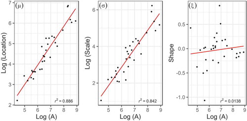
As a first step, we assessed, on the basis of maximum likelihood estimates (MLEs), whether our modelling assumptions – namely, the scaling behaviour of the GEV parameters and the existence of a spatial distribution for the shape counterpart – hold in our study area. Regarding the parameters’ scaling behaviour, it is possible to infer, from the left and middle panels in Fig. 2, that a log-log linear functional relationship between the location and the scale parameters ($\mu$ and $\sigma$, respectively) and the catchments’ drainage areas is plausible and the inclusion of such a covariate would lead to the identification of regression models with suitable predictive skills. Yet a non-negligible partition of the scatters of $\mu$ and $\sigma$ (~11% and 16%, respectively) is left unaccounted for by the regression models and must then be accommodated in the regression errors. As for the shape parameter, $\xi$ (right panel of Fig. 2), no functional pattern could be identified in the scatterplot, indicating that, in agreement with Lima et al. (2016) and Wu et al. (2018, 2019), the scaling law is not valid for this quantity.

Figure 2. Scaling behaviour of the generalized extreme value (GEV) parameters with the catchment drainage areas

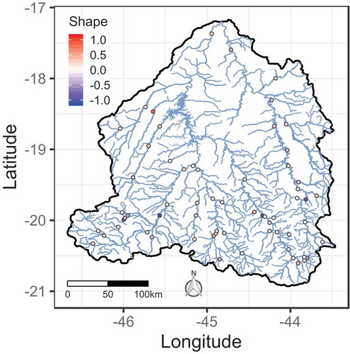
Next, to evaluate the existence of a spatial distribution of the GEV shape parameter, as resulting from the distinctions in terrain and precipitation regimes, we plotted the MLEs for $\xi$, at each site, in Fig. 3. One may note that there are somewhat well-defined groups in the southern and north-eastern portions of the study area, and roughly two others in the western part, suggesting some degree of spatial pooling for the estimates of $\xi$. Obviously, given the acknowledged difficulties in estimating such a parameter in at-site frequency analysis, particularly in those sites with small samples (see the discussion in Lima et al. 2016), the use of MLEs for $\xi$ may introduce some bias in the formation of these groups. However, since spatial patterns could be established, we believe that is reasonable to assume a variogram-based model to describe the random field that governs the spatial variation of the referred parameter.

Figure 3. Generalized extreme value shape parameter maximum likelihood estimates (MLEs) in the study region

With empirical evidence that our modelling assumptions are acceptable, we proceeded to the inference of the BHM parameters. To explore the joint posterior distributions of the parameters of models M1 and M2, we defined our sampling setup with four chains containing 5000 iterations each. The first halves of the samples in each chain were discarded as a warm-up period (Stan Development Team 2020), which resulted in final samples of 10,000 for the parameters of each model. In order to assess the convergence to the equilibrium distribution, we evaluated the $\hat{R}$ statistic and the effective sample sizes (ESSs), as proposed by Vehtari et al. (2019). Following their recommendations, we assumed that at least 400 ESSs for the four chains and the threshold $\hat{R}<1.01$ are necessary to ensure convergence.

The posterior distributions of some parameters, for models M1 and M2, are depicted in Fig. 4. General comments can be made regarding the presented results. First, with respect to the regression models for $\mu$ and $\sigma$, the regression parameters’ distributions are unimodal and approximately symmetric. Those of the regression errors’ marginal variances, in turn, despite presenting a single mode, are strongly skewed to the right. Second, for both BHMs being evaluated, the distributions of the regression parameters are shifted along the horizontal axis – which can be, at least to some extent, ascribed to the formal description of the spatial dependence structure in model M1, but their posterior variances are not much different. Finally, the marginal variances for the regression errors inferred for model M1 are, in general, larger than those for M2, which reflects, to a great extent, the more complex interactions between the regression errors and the regression parameters in the spatially dependent model, resulting in more uncertain estimates.

Figure 4. Posterior estimates of regression parameters. $\mu$, $\sigma$ and $\xi$ are, respectively, location, scale and shape parameters

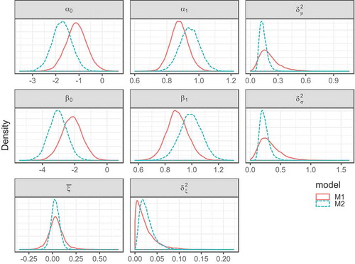
As for parameter $\bar{\xi }$, similar and relatively close to zero posterior mean values were obtained for both M1 and M2. On the other hand, the variance was smaller for the latter model. In fact, for M2, the “shrinkage” effect was more noticeable, with the 95% credible limits for $\bar{\xi }$ranging from −0.05 to 0.12, approximately. Alternatively, for M1, a broader range, from about −0.12 to 0.22, was observed for $\bar{\xi }$, which probably stemmed from the interactions of regression errors in this modelling variant. The marginal variances of the regression errors, on the other hand, were smaller in model M1, possibly due to $\bar{\xi }$ accommodating a larger part of the uncertainty.

To further investigate the implications of prescribing a formal spatial dependence structure, we computed the correlations among the regression errors and the regression parameters, and those among the regression errors and their marginal variances. Results are depicted in Fig. 5. It is possible to observe that, for the regression parameters of model M2, both the intercepts (${\alpha }_0$ and ${\beta }_0$) and the slopes (${\alpha }_1$ and ${\beta }_1$) are moderately correlated with the regression errors. Also, it appears that they are related in such a way that, after accounting for the covariates’ contribution (i.e. the intercept), a random scatter of the regression residuals would still result. Hence, we hypothesize that the somewhat more constrained inferences of the marginal variances in M2 arise in order to induce the “independence” of the regression errors – which is supported by the findings of Kjeldsen and Jones (2009) but may not accurately reflect the latent physical processes that drive the spatial variation of the GEV parameters.

Figure 5. Correlations among the parameters of the spatially dependent model (M1) and the spatially independent model (M2), and the corresponding regression errors

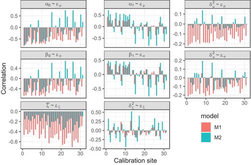
For model M1, the independence requirement is relaxed and, as a result, narrower ranges for the slopes may stem from and, to some extent, be compensated by structured scatters of the residuals once the covariates’ influence is accounted for. Consequently, the correlations among the regression slopes, ${\alpha }_1$ and ${\beta }_1$, and the corresponding regression errors are much weaker, as opposed to those associated with the intercepts ${\alpha }_0$ and ${\beta }_0$, suggesting that the latter would then induce functional patterns for the scatter of the residuals by translating the regression line. Moreover, changes in the intercepts’ values cause the regression errors to be forced in a single and opposite “direction” in response, which could then explain the larger variances of the regression parameters.

It is also possible to note that, for M2, the regression errors of the GEV shape parameter are only moderately correlated with the estimates of $\bar{\xi }$, which could be ascribed to its small posterior variance. They are, however, more strongly dependent on the marginal variances. In this case, the regional heterogeneity related to the GEV shape parameter, $\xi$, is almost entirely accommodated in the posterior marginal variance ${\delta }_{\xi }^2$. For model M1, the regression errors are much more strongly related to the estimates of $\bar{\xi }$ than to those of the marginal variances, which, in turn, suggests that the less visible “shrinkage” effect is, to some extent, attenuated by the regression errors.

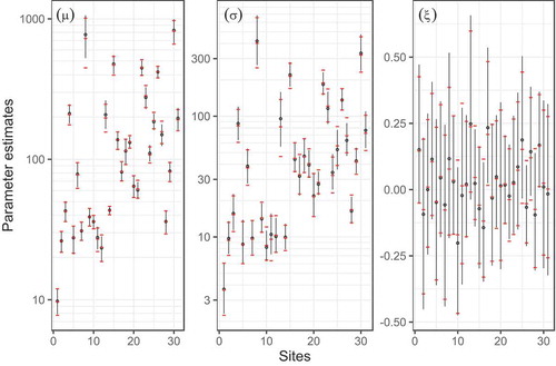
Figure 6 depicts the posterior point estimates, along with the 95% credible limits, from the calibration dataset for the GEV parameters at the gauged sites. One may note that, despite the quite distinct posterior distributions of the parameters of the regression models, no marked differences were verified from those of the parent distribution for M1 and M2. In a few sites, (e.g. 8 and 13), model M1 inferred notably narrower credible intervals for the GEV location and the scale parameters. On the other hand, utilizing M2 resulted in slightly narrower credible intervals for the shape parameter in most sites. To some extent, this similarity in estimates reinforces our conjecture that, during calibration, the effects of the unaccounted spatial dependency are accommodated in the parameters of the regression models (which could then be interpreted as systematic error components). As a result, at least on the basis of our results, the increased complexity of the spatially dependent M1 does not seem to be justified for estimation at gauged sites since the obtained quantile curves and credible intervals are virtually identical for both models. However, a more coherent representation of the spatial fields along the river network may lead to distinct results, and this certainly requires further investigation.

Figure 6. Posterior estimates of the generalized extreme value (GEV) parameters under models M1 and M2. Model M1 point estimates and 95% credible bounds are indicated, respectively, by black circles and vertical black lines; Model M2 point estimates and their 95% credible intervals are indicated by red dashes

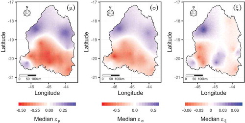
We now turn our attention to prediction at ungauged sites. For this, we first examined whether a consistent spatial behaviour for the regression errors can be established. As previously noted, most gauging stations utilized in calibration are located in the southern portion of the study area. As a result, the regression errors in points that are farther away from this densely gauged area should not be strongly affected by those inferred at the gauged sites. As a means of assessing the outlined behaviour, we estimated the predictive distribution of the regression errors in a set of 3116 points, setting them 3ʹ apart from each other, along the study area. Results are shown in Fig. 7 (in terms of median errors). One may note that clear spatial patterns arise for the regression errors of the three GEV parameters, which suggests that the proposed dependency structure could be useful for information transfer, with a possible reduction of the predictive uncertainty, mainly in the southern portion of the catchment.

Figure 7. Spatial predictive distribution of the regression errors

Finally, we estimated the quantile curves, along with the 95% credible intervals, at the validation sites. Results are summarized in the panels of Fig. 8. Some remarks can be made regarding these panels. First, the median quantile curves in panels (a) and (b), as obtained from model M1, closely resemble their empirical counterparts. Those for model M2, in turn, incurred a lack of fit, overestimating most of the empirical quantiles. In addition, the 95% credible intervals inferred from M1 are much narrower than those stemming from M2, suggesting that more reliable estimates were obtained when the spatial dependency structure was considered, due to the smaller predictive variances. It may be argued that validation sites 1 and 2 are located in densely gauged areas, which would certainly favour the more complex model. However, the obtained results provide evidence that, when information is available in catchments close to the ungauged target site, accommodating the spatial correlation in model parameters, even under a simple model such as a variogram, is beneficial when predicting floods at these locations.

Figure 8. Quantile curves of the validation sites and their 95% credible intervals estimated by models M1 and M2

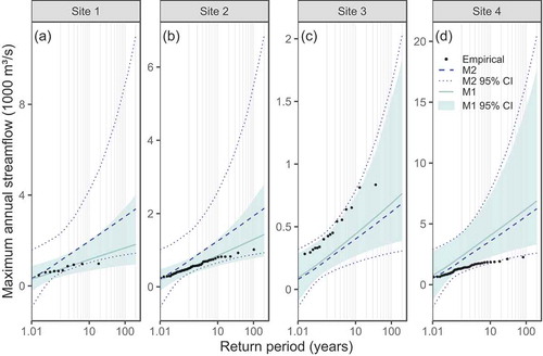
Panels (c) and (d), in turn, show predictions in poorly gauged areas. In fact, sites 3 and 4 present a small number of neighbours, and those are relatively distant from the target catchments, which potentially explains the degraded performance of the spatially dependent model in these locations. In site 3, despite the evidence of a lack of fit with respect to point quantile estimates, there is still some indication that model M1 performed best, as most empirical quantiles were enclosed (or are very close to the upper uncertainty bands) by its slightly narrower credible intervals. Site 4, in turn, favours model M2, whose wider credible intervals were able to enclose a considerably larger number of empirical quantiles. These facts suggest that M2 may become more effective than M1 as the number of nearby gauging stations decreases. In other words, the more “conservative” estimates of the predictive uncertainty provided by the spatially independent model are more likely to properly account for maximum floods’ random variability in poorly gauged areas. To a great extent, this highlights the difficulty of reliably performing RFFA in regions with scarce hydrological information despite the use of more and more complex models.

4 Conclusions

This paper explored an extension of the partial pooling hierarchical approach for GEV-based regional flood frequency analysis (Lima et al. 2016) by considering spatial dependency structures for the distribution parameters. In short, the scaling law is utilized to regress the GEV location and scale parameters against the catchments’ drainage areas, whereas the shape parameter in each site is assumed to “shrink” towards a mean regional value. The spatial dependency structure is formally established on the basis of Gaussian random fields and introduced in the process level of the hierarchical model through the regression errors.

The application of the proposed approach to a set of streamflow gauging stations in the Alto do São Francisco River catchment provided some interesting insights regarding the effects of incorporating the spatial dependency in the GEV parameters. First, at gauged sites, ignoring the spatial correlation entailed somewhat distinct estimates, in terms of posterior distributions, for the regression parameters. However, the estimates of the GEV parameters were remarkably similar, which suggests that, at least to some extent, the regression errors accommodate the modelling bias during inference. Of course, utilizing a more coherent representation of the spatial dependency structure, as opposed to variograms (e.g. Müller and Thompson 2015), could alter the outlined posterior behaviour and highlight potential advantages of the spatially dependent approach – mainly, the more realistic description of the physical phenomena that govern the probabilistic behaviour of floods at the regional scale. However, our results suggest that estimation at gauged sites is not strongly affected by the increased complexity of the proposed spatial model, and a simpler alternative should suffice if interest lies solely in increasing the reliability of extreme quantile estimation in these locations.

At ungauged sites, the benefits of formally describing the spatial behaviour of the GEV parameters are more noticeable when information from nearby sites is available. In fact, for sites with a number of close neighbours, both accuracy and precision were strongly improved in the prediction step. As a result, in densely or moderately densely gauged regions, the more complex structure of the spatially dependent model should be justified. However, for those locations distant from gauged sites, predictions of both models prompted a lack of fit with respect to point estimates and led to very large credible intervals. In effect, it appears that, at least on the basis of this case study, the proposed dependency structure is not effective for accounting for the maximum floods’ variability in cases with low availability of information from nearby sites. This fact reinforces our conjecture that a more coherent description of the spatial fields is necessary, and should encourage more research developments in spatial processes for improving estimation and prediction.

At last, the proposed framework can, for certain, be further investigated and improved by tackling some of its limiting assumptions. First, due to our simplified approach for preserving the physical consistency of the regression models, the levels of spatial correlation among flood observations were relatively low. The conditional independence assumption, however, may not be realistic when the river hierarchy is properly taken into account during inference. Hence, a suitable account of data dependence at the likelihood level (e.g. Davison et al. 2013) might also be necessary to allow a better description of the spatial dependence within the study region. Furthermore, we did not evaluate how the introduction of cross-correlation among the regression errors related to distinct GEV parameters in process specification (e.g. Kim et al. 2018) may influence inference procedures, and this is still open for investigation.

Acknowledgements

The authors thank the associate editor and the two anonymous reviewers for their valuable comments and suggestions that greatly helped us to improve the manuscript.

Disclosure statement

No potential conflict of interest was reported by the authors.

Additional information

Funding

This study was financed in part by the Coordenação de Aperfeiçoamento de Pessoal de Nível Superior – Brasil (CAPES) – Finance Code 001.

References

- Ahani, A., Nadoushani, S.M., and Moridi, A., 2020. Simultaneous regionalization of gauged and ungauged watersheds using a missing data clustering method. Journal of Hydrologic Engineering, 25 (5), 04020015. doi:10.1061/(ASCE)HE.1943-5584.0001916
- Ahn, K. and Palmer, R., 2016. Regional flood frequency analysis using spatial proximity and basin characteristics: quantile regression vs. parameter regression technique. Journal of Hydrology, 540, 515–526. doi:10.1016/j.jhydrol.2016.06.047
- Ahn, K., Palmer, R., and Steinschneider, S., 2017. A hierarchical Bayesian model for regionalized seasonal forecasts: application to low flows in the northeastern United States. Water Resources Research, 53 (1), 503–521. doi:10.1002/2016WR019605
- Ahn, K. and Steinschneider, S., 2019. Hierarchical Bayesian model for streamflow estimation at ungauged sites via spatial scaling in the Great Lakes basin. Journal of Water Resources Planning and Management, 145 (8), 04019030. doi:10.1061/(ASCE)WR.1943-5452.0001091
- Alexander, R.B., Schwarz, G.E., and Boyer, E.W., 2019. Advances in quantifying streamflow variability across continental scales: 2. Improved model regionalization and prediction uncertainties using hierarchical Bayesian methods. Water Resources Research, 55 (12), 11061–11087. doi:10.1029/2019WR025037
- ANA (Agência Nacional de Águas), 2003. Projeto de Gerenciamento Integrado das Atividades Desenvolvidas em Terra na Bacia do São Francisco, Sub-projeto 4.5.A – diagnóstico Analítico da Bacia e sua Zona Costeira. Brasília: ANA.
- Baker, V.R., et al., 2003. A bright future for old flows: origin, status and future paleoflood hydrology. In: V.R. Thorndycraft, ed. Proceedings of the 2002 PHEFRA workshop – Paleofloods, historical floods and climatic variability: applications in flood risk assessment, Madri: Centro de Ciencias Medioambientales, 13–18.
- Basu, B. and Srinivas, V.V., 2016. Evaluation of the index-flood approach related regional frequency analysis procedures. Journal of Hydrologic Engineering, 21 (1), 04015052. doi:10.1061/(ASCE)HE.1943-5584.0001264
- Bezac, N., Brilly, M., and Sraj, M., 2014. Comparison between the peaks-over-threshold method and the annual maximum method for flood frequency analysis. Hydrological Sciences Journal, 59 (5), 595–977. doi:10.1080/02626667.2013.831174
- Botero, B.A. and Frances, F., 2010. Estimation of high return period flood quantiles using additional non-systematic information with upper bounded statistical models. Hydrology and Earth System Sciences, 14, 2617–2628. doi:10.5194/hess-14-2617-2010
- Bracken, C., et al., 2016. Spatial Bayesian hierarchical modeling of precipitation extremes over a large domain. Water Resources Research, 52 (8), 6643–6655. doi:10.1002/2016WR018768
- Coles, S.G., 2001. An introduction to statistical modeling of extreme events. London: Springer. doi:10.1007/978-1-4471-3675-0
- Cooley, D., Nychka, D., and Naveau, P., 2007. Bayesian spatial modeling of extreme precipitation return levels. Journal of the American Statistical Association, 102 (479), 824–840. doi:10.1198/016214506000000780
- Costa, V. and Fernandes, W., 2017. Bayesian estimation of extreme flood quantiles using a rainfall-runoff model and a stochastic daily rainfall generator. Journal of Hydrology, 554, 137–154. doi:10.1016/j.jhydrol.2017.09.003
- CPRM, 2001. Regionalização de Vazões das Sub-bacias 40 e 41 – Alto São Francisco. Belo Horizonte: ANEEL/CPRM.
- Dalrymple, T., 1960. Flood frequency analyses. Washignton, DC: US Geological Survey Water-Supply Paper Bi. 1543-A, 80.
- Davison, A.C., Huser, R., and Thibaud, E., 2013. Geostatistics of dependent and asymptotically independent extremes. Mathematical Geosciences, 45 (5), 511–529. doi:10.1007/s11004-013-9469-y
- Dyrrdal, A.V., et al. 2015. Bayesian hierarchical modeling of extreme hourly precipitation in Norway. Environmetrics, 26 (2), 89–106. doi:10.1002/env.2301
- Fernandes, W., Naghettini, M., and Loschi, R., 2010. A Bayesian approach for estimating extreme flood probabilities with upper-bounded distribution functions. Stochastic Environmental Research and Risk Assessment, 24 (8), 1127–1143. doi:10.1007/s00477-010-0365-4
- Gupta, V.K. and Dawdy, D.R., 1995. Physical interpretations of regional variations in the scaling exponents of flood quantiles. Hydrological Processes, 9 (3–4), 347–361. doi:10.1002/hyp.3360090309
- Gupta, V.K., Mesa, O.J., and Dawdy, D.R., 1994. Multiscaling theory of flood peaks: regional quantile analysis. Water Resources Research, 30 (12), 3405–3421. doi:10.1029/94WR01791
- Gupta, V.K., Troutman, B.M., and Dawdy, D.R., 2007. Towards a nonlinear geophysical theory of floods in river networks: an overview of 20 years of progress. In: A. Tsonis and J. Elsner, eds. Nonlinear dynamics in geosciences. New York: Springer, 121–151.
- Gupta, V.K. and Waymire, E., 1990. Multiscaling properties of spatial rainfall and river flow distributions. Journal of Geophysiscal Research, 95 (D3), 1999–2009. doi:10.1029/JD095iD03p01999
- Hailegeorgis, T.T. and Alfredsen, K., 2017. Regional flood frequency analysis and prediction in ungauged basins including estimation of major uncertainties for mid-Norway. Journal of Hydrology: Regional Studies, 9, 104–126. doi:10.1016/j.ejrh.2016.11.004
- Hall, J. and Solomatine, D., 2008. A framework for uncertainty analysis in flood risk management decisions. International Journal of River Basin Management, 6 (2), 85–98. doi:10.1080/15715124.2008.9635339
- He, J., Anderson., A., and Valeo, C., 2015. Bias compensation in flood frequency analysis. Hydrological Sciences Journal, 60 (3), 381–401. doi:10.1080/02626667.2014.885651
- Hoffman, M.D. and Gelman, A., 2014. The No-U-Turn sampler: adaptively setting path lengths in Hamiltonian Monte Carlo. Journal of Machine Learning Research, 15, 1593–1623.
- Hosking, J.R.M. and Wallis, J.R., 1997. Regional frequency analysis: an approach based on L-moments. Cambridge: Cambridge University Press, 224. doi:10.1017/CBO9780511529443
- Ishak, E., et al., 2011. Scaling property of regional floods in New South Wales Australia. Natural Hazards, 58 (3), 1155–1167. doi:10.1007/s11069-011-9719-6
- Jenkinson, A.F., 1955. The frequency distribution of the annual maximum (or minimum) of meteorological elements. Quarterly Journal of the Royal Meteorological Society, 81 (348), 158–171. doi:10.1002/qj.49708134804
- Jesus, L.F.L., Costa, V., and Fernandes, W., 2020. Evaluating the influence of extending hydrologic time series in extreme quantile estimation. Water and Environment Journal, (S1), in press. doi:10.1111/wej.12579
- Khali, B. and Adamowski, J., 2014. Evaluation of the performance of eight record-extension techniques under different levels of association, presence of outliers and different sizes of concurrent records: A Monte Carlo study. Water Resources Management, 28 (14), 5139–5155. doi:10.1007/s11269-014-0799-4
- Khalil, B., et al., 2016. A novel record-extension technique for water quality variables based on L-moments. Water Air Soil Poll, 227 (6), 1–20. doi:10.1007/s11270-016-2852-9
- Kim, T., Kwon, H., and Lima, C., 2018. A Bayesian partial pooling approach to mean field bias correction of weather radar rainfall estimates: application to Osungsan weather radar in South Korea. Journal of Hydrology, 565, 14–26. doi:10.1016/j.jhydrol.2018.07.082
- Kjeldsen, T.R. and Jones, D., 2007. Estimation of an index flood using data transfer in the UK. Hydrological Sciences Journal, 52 (1), 86–98. doi:10.1623/hysj.52.1.86
- Kjeldsen, T.R. and Jones, D.A., 2009. An exploratory analysis of error components in hydrological regression modeling. Water Resources Research, 45 (2), W02407. doi:10.1029/2007WR006283
- Kwon, H., Brown, C., and Lall, U., 2008. Climate informed flood frequency analysis and prediction in Montana using hierarchical Bayesian modeling. Geophysical Research Letters, 35 (5), L05404. doi:10.1029/2007GL032220
- Lima, C.H.R., et al., 2016. A hierarchical Bayesian GEV model for improving local and regional flood quantile estimates. Journal of Hydrology, 541, 816–823. doi:10.1016/j.jhydrol.2016.07.042
- Lima, C.H.R. and Lall, U., 2010. Spatial scaling in a changing climate: A hierarchical Bayesian model for non-stationary multi-site annual maximum and monthly streamflow. Journal of Hydrology, 383 (3–4), 307–318. doi:10.1016/j.jhydrol.2009.12.045
- Martins, E. and Stedinger, J., 2000. Generalized maximum‐likelihood generalized extreme‐value quantile estimators for hydrologic data. Water Resources Research, 36 (3), 737–744. doi:10.1029/1999WR900330
- McClymont, K., et al., 2019. Flood resilience: a systematic review. Journal of Environment Planning and Management. doi:10.1080/09640568.2019.1641474
- McMillan, H., et al., 2017. How uncertainty analysis of streamflow data can reduce costs and promote robust decisions in water management applications. Water Resources Research, 53 (7), 5220–5228. doi:10.1002/2016WR020328
- Morrison, J.E. and Smith, J.A., 2002. Stochastic modeling of flood peaks using the generalized extreme value distribution. Water Resources Research, 38 (12), 1–12. doi:10.1029/2001WR000502
- Müller, M.F. and Thompson, S.E., 2015. TopREML: a topological restricted maximum likelihood approach to regionalize trended runoff signatures in stream networks. Hydrology and Earth System Sciences, 19 (6), 2925–2942. doi:10.5194/hess-19-2925-2015
- Naghettini, M., 2017. Fundamentals of statistical hydrology. Cham: Springer Internation Publishing.
- Najafi, M.R. and Moradkhani, H., 2013. Analysis of runoff extremes using spatial hierarchical Bayesian modeling. Water Resources Research, 49 (10), 6656–6670. doi:10.1002/wrcr.20381
- Northrop, P.J., 2004. Likelihood-based approaches to flood frequency estimation. Journal of Hydrology, 292 (1–4), 96–113. doi:10.1016/j.jhydrol.2003.12.031
- O’Brien, N.L. and Burn, D.H., 2014. A nonstationary index-flood technique for estimating extreme quantiles for annual maximum streamflow. Journal of Hydrology, 519, 2040–2048. doi:10.1016/j.jhydrol.2014.09.041
- Renard, B., 2011. A Bayesian hierarchical approach to regional frequency analysis. Water Resources Research, 47 (11), 1–21. doi:10.1029/2010WR010089
- Sene, K.J., Houghton-Carr, H.A., and Hachache, A., 2001. Preliminary flood frequency estimates for Lebanon. Hydrological Sciences Journal, 46 (5), 659–676. doi:10.1080/02626660109492863
- Silva, A., et al., 2017. A Bayesian peaks-over-threshold analysis of floods in the Itajaí-açu River under stationarity and nonstationarity. Stochastic Environmental Research and Risk Assessment (Print), 31 (1), 185–204. doi:10.1007/s00477-015-1184-4
- Silva, A.T., Naghettini, M., and Portela, M.M., 2016. On some aspects of peaks-over-threshold modeling of floods under nonstationarity using climate covariates. Stochastic Environmental Research and Risk Assessment (Print), 30 (1), 207–224. doi:10.1007/s00477-015-1072-y
- Silva, A.T., Portela, M.M., and Naghettini, M., 2014. On peaks-over-threshold modeling of floods with zero-inflated poisson arrivals under stationarity and nonstationarity. Stochastic Environmental Research and Risk Assessment (Print), 28 (6), 1587–1599. doi:10.1007/s00477-013-0813-z
- Stan Development Team, 2020. RStan: the R interface to Stan. R package version 2.19.3. Retrieved from http://mc-stan.org/.
- Thorarinsdottir, T.L., et al., 2018. Bayesian regional flood frequency analysis for large catchments. Water Resources Research, 54 (9), 6929–6947. doi:10.1029/2017WR022460
- Tyralis, H., Papacharalampous, G., and Sarintip, T., 2019. How to explain and predict the shape parameter of the generalized extreme value distribution of streamflow extremes using a big dataset. Journal of Hydrology, 574, 628–645. doi:10.20944/preprints201811.0265.v1
- Vehtari, A., et al., 2019. Rank-normalization, folding, and localization: an improved R for assessing convergence of MCMC [online]. Available from: http://arxiv.org/abs/1903.08008v2 [Accessed 3 March 2020].
- Villarini, G., et al., 2011. Analyses of seasonal and annual maximum daily discharge records for central Europe. Journal of Hydrology, 399 (3), 299–312. doi:10.1016/j.jhydrol.2011.01.007
- Villarini, G., Smith, J.A., and Napolitano, F., 2010. Nonstationary modeling of a long record of rainfall and temperature over Rome. Advances in Water Resources, 33 (10), 1256–1267. doi:10.1016/j.advwatres.2010.03.013
- Wu, Y., et al., 2018. Local and regional flood frequency analysis based on hierarchical Bayesian model: application to annual maximum streamflow for the Huaihe River basin. Hydrology and Earth System Sciences Discussions, 1–21. doi:10.5194/hess-2018-22
- Wu, Y., Xue, L., and Liu, Y., 2019. Local and regional flood frequency analysis based on hierarchical Bayesian model in Dongting Lake Basin, China. Water Science and Engineering, 12 (4), 253–262. doi:10.1016/j.wse.2019.12.001
- Yan, H. and Moradkhani, H., 2015. A regional Bayesian hierarchical model for flood frequency analysis. Stochastic Environmental Research and Risk Assessment, 29 (3), 1019–1036. doi:10.1007/s00477-014-0975-3
- Yan, H. and Moradkhani, H., 2016. Toward more robust extreme flood prediction by Bayesian hierarchical and multimodeling. Natural Hazards, 81 (1), 203–225. doi:10.1007/s11069-015-2070-6