Hydrological responses to human-induced land use/land cover changes in the Gidabo River basin, Ethiopia

ABSTRACT

Land-use/land-cover (LULC) changes in the Gidabo basin, Rift Valley, Ethiopia, have greatly affected the hydrology of the basin. This study integrates hydrological modelling with statistical analysis to evaluate the hydrological response of LULC changes during the period 1988–2018. Using the Soil and Water Assessment Tool (SWAT) and partial least squares regression (PLSR) models, the influences of individual LULC changes on different components of the hydrological cycle are assessed. The results of the Mann-Kendall test showed no significant trends in annual rainfall over the basin at the 95% significance level. Change in LULC resulted in an increase in annual mean surface runoff by 23.6 mm during the period 1988–2018. Meanwhile, the annual mean baseflow, lateral flow, percolation and evapotranspiration (ET) were reduced by 9.1, 4.2, 10.2 and 12.2 mm, respectively. PLSR analysis indicated that cultivated land affected the lateral flow and ET negatively in contrast to agroforestry and grassland, which had a positive influence.

KEYWORDS:

• Gidabo watershed
• Ethiopia
• land-use/land-cover (LULC) change
• hydrological components
• Soil and Water Assessment Tool (SWAT)
• partial least squares regression (PLSR) model

Editor S. Archfield Associate Editor V. Samadi

1 Introduction

Water is one of the most important natural resources on which all living things thrive. It goes through a system of circulation among ocean, atmosphere and land, known as the hydrological cycle (Chow et al. 1988). The changing land-use/land-cover (LULC) and climate affect various components of the hydrological cycle and, consequently, the water resources in a river basin (Zhang et al. 2016). Human-induced LULC changes influence the hydrological processes (Gebremicael et al. 2019) such as interception rates, soil moisture storage, evapotranspiration (ET) loss, infiltration and groundwater recharge, leading to modifications in basin water resources (Gebremicael et al. 2013, Ayele et al. 2017, Gashaw et al. 2018). These changes amend vegetation cover and surface roughness affecting the timing and magnitude of surface runoff and groundwater recharge, leading to modifications in streamflow and magnitude/frequency of floods (Zhang et al. 2016). As an example, conversion or amendment of forest into urban and agricultural area results in higher surface runoff and reduced groundwater recharge (Baker and Miller 2013, Gyamfi et al. 2016).

Hydrological models are generally used to evaluate the effects of LULC changes on hydrological processes. These models simulate the spatial as well as temporal responses of various LULC changes on the hydrological components in a river basin (Zhou et al. 2013, Gashaw et al. 2018, Yan et al. 2018, Garg et al. 2019, Liyew et al. 2019b). Using such hydrological models, a number of studies have evaluated the hydrological response to environmental changes at the watershed level. However, at different spatial and temporal scales, the predominant factors and the degree to which LULC changes influence the hydrological conditions often vary. Spatially, the impact of LULC changes on hydrology is commonly more evident at a sub-basin scale (Wagner et al. 2013, Schilling et al. 2014, Marhaento et al. 2017), while their impact on the water budget elements is relatively small at a larger basin scale due to compensating effects (Schilling et al. 2014, Shawul et al. 2019). For water resource managers, information about how, and by how much, LULC changes will influence water availability at the sub-basin level is more relevant for planning appropriate mitigation measures (Marhaento et al. 2017). As such, research is required at the sub-basin level to better realize the responses of hydrological conditions to LULC changes.

In addition to quantifying the impacts of gross LULC changes on hydrological components using a hydrological model, it is also important to scrutinize the effect and contribution of each LULC change on different hydrological components of a catchment (Shi et al. 2013, Yan et al. 2013, Gashaw et al. 2018, Gebremicael et al. 2019, Shawul et al. 2019). The partial least squares regression (PLSR) model is an advanced multivariate statistical method that is useful to investigate the interaction of individual LULC classes (independent variable) with different hydrological components (dependent variables) (Carrascal et al. 2009, Fang et al. 2015, Shawul et al. 2019). The PLSR approach is a useful tool to ascertain whether the observed change in LULC is large enough to cause the change in hydrological processes, and it can be applied to zoom in on the LULC class responsible for the change in hydrological elements (Gebremicael et al. 2019). Further, this technique is suitable for solving multicollinearity problems, an issue that arises when at least two predictors (independent variables) in the model are correlated (Abdi 2010, Shi et al. 2013).

In Ethiopia, anthropogenic activities have affected the availability of water resources in river basins (Ayele et al. 2017, Liyew et al. 2019b). Intensive grazing, deforestation and extraordinary cultivation practices are some key alterations in the catchments that have modified the hydrological processes (Legesse et al. 2003, Ayele et al. 2017) and devastated not only the highland areas, due to enhanced erosion and reduction in crop yields (Setegn et al. 2009, Liyew et al. 2019a), but also the water channels and storage because of sedimentation (Setegn et al. 2009). Several studies reported the effects of LULC changes on hydrology in Ethiopia (e.g. Legesse et al. 2003, Gebremicael et al. 2013, Gashaw et al. 2018, Liyew et al. 2019b). Gashaw et al. (2018) reported enhanced cultivated and built-up areas at the cost of forest, shrubland and grassland during 1985–2015 in Andassa watershed, Blue Nile Basin, Ethiopia. As a result, surface runoff and water yield were amplified while lateral flow, groundwater flow and ET diminished. Gebremicael et al. (2013) conducted a trend analysis of runoff and sediment fluxes in the Upper Blue Nile Basin by a combination of statistical testing and hydrological modelling, and found that the rainfall over the basin did not change significantly during 1970–2005 although surface runoff increased due to land-use changes in the basin.

As only a few studies have been attempted to link the LULC changes to hydrological components using coupled hydrological and PLSR models (Gebremicael et al. 2019, Shawul et al. 2019), the primary objective of this study is to quantify the contribution of changes in individual LULC classes to changes in components of water balance using the combination of a hydrological model (the Soil and Water Assessment Tool or SWAT) and the PLSR model. The Gidabo watershed, Rift Valley Basin, Ethiopia, has been selected for the study; it is one of the most profitable areas in the basin and suffers from human-induced resource degradation because of the increased cultivated land and unregulated LULC alterations, along with the booming population growth. The impact of such LULC changes on hydrological components are poorly studied in this basin, and such information may be vital for developing sustainable water resource management plans for the basin.

2 Study area

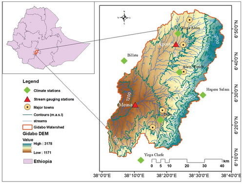
The Gidabo watershed (Fig. 1) is located in the Abaya-Chamo sub-basin of the Rift Valley Basin in Ethiopia. The River Gidabo twists through forested and agricultural land of the escarpment and rift floor, finally ending in Lake Abaya, the biggest lake in the Rift Valley (Mechal et al. 2015). The river is around 120 km long, with an estimated catchment area of 3097 km². The topographical area begins from the northeastern piles of Soka Sonicha and lies in the range 6.11 to 6.58°N and 38.0 to 38.38°E. In particular, the basin lies in the Sidama and Gedeo Zones of the Southern Nation Nationalities and People of Regional State (SNNPRS) and the Borena Zone of Oromiya Regional State. The altitude of the basin ranges from 3178 m at the most elevated point to 1171 m at the outlet. The pattern of rainfall in the area has four seasons, namely the high rainy season (April and May), moderate rainy season (September to October), low rainy season (July and August) and dry season (November to February) (Belihu et al. 2018). The mean annual rainfall in the basin is 1385 mm and the average monthly temperature varies from 11 to 25°C.

Figure 1. Location map of the study area showing Gidabo watershed, stream gauging stations, climate stations, contours and streams

Note. DEM: digital elevation model; m.a.s.l: meter above sea level.

3 Data availability

The dataset required for the SWAT model setup includes a digital elevation model (DEM), soil map, LULC map and the climate data. The Shuttle Radar Topographic Mission (SRTM) DEM from the US Geological Survey (USGS) Earth Explorer (https://earthexplorer.usgs.gov), with 30 m × 30 m resolution, was processed in ArcGIS and used in this study. Images from the Landsat satellite (Table 1) were downloaded from the USGS Earth Explorer. The satellite images were taken during the dry season (January–February) and carefully chosen based on the data availability and cloud conditions in the catchment. Ground truth points in the study area, used for classification and evaluation of accuracy, were gathered from field surveys, Google Earth, countrywide LULC maps and the literature. The soil map was collected from the Ministry of Agriculture, Ethiopia, while the soil properties were derived from the latest irrigation design and feasibility study report (WWDSE 2007) for the basin and the harmonized World Soil Database (http://www.fao.org/soils-portal/soil-survey/soil-maps-and-databases/harmonized-world-soil-database-v12/en/).

Table 1. Explanation of satellite images used in this study. TM: Thematic mapper; ETM+: Enhanced thematic mapper plus; m: meter

Satellite	Sensor	Path/row	Resolution (m)	Acquisition date
Landsat 5	TM Multispectral	168/55/56	30	28 February 1988
Landsat 7	ETM+ Multispectral	168/55/56	30	5 February 2000
Landsat 8	Operational Land Imager (OLI)	168/55/56	30	29 January 2018

The SWAT model requires daily meteorological data as input. Therfore, the daily precipitation data, and maximum and minimum daily temperature data, for eight stations from 1987 to 2018 were obtained from the National Meteorological Services Agency of Ethiopia. After analysing the data, six rainfall stations and five temperature stations were selected. The observed daily streamflows of two gauging sites were obtained from the Ministry of Water, Irrigation and Electricity of Ethiopia for model calibration and validation. Finally, all the input data for the study basin were processed for input to the SWAT model.

4 Methodology adopted

4.1 Trend and change-point analysis

Assessing the presence of trends in hydro-climatological variables is vital for distinguishing and understanding changes in hydrological elements (Tekleab et al. 2013). The Mann-Kendall (MK) test (Mann 1945, Kendall 1975) was carried out to check the rainfall trends in the study area. The MK test is a rank-based, non-parametric statistical test applied in numerous hydro-climatological studies for detecting monotonic trends in time series data (Tekleab et al. 2013, Belihu et al. 2018). The Pettitt (1979) test was applied to detect the change points in rainfall trends. It is one of the most important statistical indicators in analysing the hydrological responses to LULC and climate change (Gebremicael et al. 2013).

4.2 Image classification and LULC change detection

For LULC change detection, Landsat images were first pre-processed to enhance the quality and visibility of features (Liyew et al. 2019a). Then, unsupervised classification was implemented to ascertain LULC groups. Finally, the maximum likelihood technique (Gashaw et al. 2017, Liyew et al. 2019a) was used for supervised classification and the majority filter was employed for post-processing.

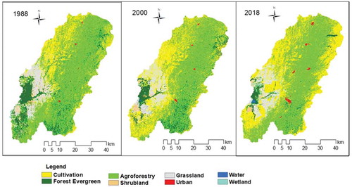
Ground truth points of 191 locations were utilized for accuracy assessment of the images from 2018. However, for the images from 1988 and 2000, 149 and 155 reference data, obtained from Google Earth, were used. Overall accuracy and Kappa statistics, derived from the error matrix, were used to evaluate the accuracy. ERDAS 2018 and ArcGIS 10.5 were used for image classification and mapping. The LULC maps for the years 1988, 2000 and 2018 are shown in Fig. 2. The rate of change of the classified LULC maps (Gashaw et al. 2017, Liyew et al. 2019a) was estimated as follows:

(1) $\mathrm{C}\mathrm{h}\mathrm{a}\mathrm{n}\mathrm{g}\mathrm{e}\mathrm{R}\mathrm{a}\mathrm{t}\mathrm{e}=\frac{A-B}{Z}$(1)

Figure 2. Land-use/land-cover maps of the study area for the years 1988, 2000 and 2018

where ChangeRate is the rate of change (km²/year); A is the area of LULC (km²) at time t − 2; B is the area of LULC (km²) at time t − 1; and Z is the time interval between A and B (years).

4.3 Description of the SWAT model

SWAT is a semi-distributed physically based simulation model that can predict the effect of climate and anthropogenic alterations on the hydrological systems in watersheds with varying soils, land-use and management conditions over long periods (Arnold et al. 1998). SWAT divides the basin into groups of similar soils, slopes and land covers, which provide similar hydrological responses, called hydrological response units (HRUs) (Neitsch et al. 2011). The model simulates the land phase processes of the hydrological components based on the following water balance equation (Arnold et al. 1998):

(2) $\mathrm{S}{\mathrm{W}}_t=\mathrm{S}{\mathrm{W}}_0+\sum _{i=1}^t\left(R_d-Q_s-E_a-W_s-Q_g\right)$(2)

where SW_t is the final soil water content (mm), SW₀ is the initial soil water content on day i (mm), t is the time (d), R_d is the amount of precipitation on day i (mm), Q_s is the amount of surface runoff on day i (mm), E_a is the amount of evapotranspiration on day i (mm), W_s is the amount of percolation and bypass flow exiting the soil profile bottom on day i (mm) and Q_g is the amount of return flow on day i (mm). Details of the model are available online (http://swatmodel.tamu.edu/).

4.4 Set-up and calibration of the SWAT model

The model SWAT Version 2012 (Neitsch et al. 2011) was used to evaluate the impacts of LULC changes on the hydrology of the Gidabo watershed. The model was set up for the study watershed using the available hydro-meteorological and spatial data. The study area was delineated in SWAT using SRTM DEM (30 m spatial resolution) with a minimum threshold drainage area of 6000 ha. Subsequently, the basin was divided into 45 sub-basins. A soil database that includes soil physical properties was prepared and imported into the SWAT databases. The LULC map, soil map and slope map were imported, overlaid and linked with the SWAT databases to define the HRUs. The slope of the basin is divided into three classes by considering the multi-slope option. As a threshold, 10% land use, 10% soil and 10% slope were used to discretize the 45 sub-basins into 409 HRUs derived from LULC, soil and slope maps. Finally, the precipitation and weather data were overlaid before writing and finalizing all input files. Then, the Soil Conservation Service (SCS) curve number (CN) (USDA-SCS 1972) method was selected to simulate surface runoff, using the Penman-Monteith (Monteith 1965) method for potential evapotranspiration and the kinematic storage method for predicting the lateral flow. Details of the model set-up are available online (see http://swatmodel.tamu.edu/).

The model is evaluated through calibration and validation (Abbaspour et al. 2017). Before calibration, the most sensitive parameters of the model for the present set-up were identified using global sensitivity analysis available in SWAT CUP (Calibration and uncertainty program) (Abbaspour et al. 2017), and the t statistic and p value (Abbaspour et al. 2007, Gashaw et al. 2018) were used to establish significance. The Sequential Uncertainty Fitting (SUFI-2) algorithm was used for calibration and validation.

In line with the suggestion of Niraula et al. (2015) and Ayele et al. (2017) for spatial evaluation, the model was calibrated using monthly flow data available for the periods 1990–2005 and 1997–2003 at the Aposto and Measa gauging sites, respectively. Subsequently, the model was validated using the flow data for the periods 2006–2014 (Aposto gauging site) and 2004–2007 (Measa gauging site). Warm-up periods in hydrological studies may range from months to decades, with 1–4 years being common for watershed-scale modeling (e.g. Mankin et al. 2010). Long warm-up periods require measured weather data before the simulation period, which may be a limitation for some applications. Hence, in this study, data for the year 1987 were used for the warm-up. The LULC map for the year 2000 was used for calibration as well as validation. Various performance evaluation criteria, such as the Nash-Sutcliffe efficiency (NSE), the coefficient of determination (R²) and percentage bias (PBIAS), were used to evaluate the performance (Moriasi et al. 2007), as given by the following equations:

(3) $\mathrm{N}\mathrm{S}\mathrm{E}=1-\frac{\sum {\left(Q_o-R_s\right)}^2}{\sum {\left(Q_o-R_a\right)}^2}$(3)

(4) $R^2=\frac{{\left(\sum \left[Q_o-Q_a\right]\left[R_s-R_a\right]\right)}^2}{\sum {\left[Q_o-Q_a\right]}^2\sum {\left[R_s-R_a\right]}^2}$(4)

(5) $\mathrm{P}\mathrm{B}\mathrm{I}\mathrm{A}\mathrm{S}=\left(\frac{\sum \left(Q_o-R_s\right)}{\sum Q_o}\right)\times 100$(5)

where R_s is the simulated flow, R_a is the mean simulated flow, Q_o is the observed flow and Q_a is the mean observed flow. All flow values are in m³/s.

4.5 Model application

To evaluate the effects of LULC changes on hydrological components at basin and sub-basin scales, simulations with the calibrated SWAT model were carried out by separately considering the LULC maps for the years 1988, 2000 and 2018 as inputs to the model.

4.6 PLSR model

The PLSR technique is an extension of multivariate analysis, which combines the features of principal component analysis and multiple regressions (Abdi 2007, 2010). It predicts a set of the dependent variable(s) from a group of predictors (Wold et al. 2001, Abdi 2007, 2010, Carrascal et al. 2009). The technique was developed for econometrics (Wold et al. 2001) and later used as a tool to analyse data from chemical applications (Mevik and Wehrens 2007) and ecological studies (Carrascal et al. 2009). Recently, the PLSR model has been used for various hydrological applications such as exploring the effects of changes in individual land-use classes on streamflow and sediment yield (Yan et al. 2013); linking soil erosion, sediment yield and the sediment delivery ratio to landscape metrics (Shi et al. 2013); investigating the effects of land-use change on runoff and suspended sediment (Fang et al. 2015), estimation of flows in urban drainage (Brito et al. 2017); and quantifying the influence of LULC classes on hydrological components (Ayele et al. 2017, Gashaw et al. 2018, Gebremicael et al. 2019, Shawul et al. 2019). PLSR is very advantageous under the following conditions: (a) when the number of predictors is similar to or higher than the number of observations; (b) for a large number of predictors; (c) for several response variables and many predictors (Carrascal et al. 2009, Abdi 2010); and (d) in helping to identify mistakes in the input data (Fang et al. 2015). Further details on the PLSR technique may be found in Wold et al. (2001), Carrascal et al. (2009) and Abdi (2010).

Assessing the hydrological responses using the hydrological model is not done to reveal the relationship of individual LULC classes with, or their influence on, components of the water budget (Gebremicael et al. 2019). Pearson correlation was applied to identify the correlation between changes in LULC classes and components of water budget at the sub-basin level at the 95% significance level. Then, the PLSR model was employed to quantify the influence of individual LULC classes on components of the water budget at the sub-basin level. PLSR relates the changes in hydrological components to the changes in LULC classes (Ayele et al. 2017, Shawul et al. 2019). It specifies the relationship between response variables, y, and predictor variables, x, as follows:

(6) $y=a+b_1{x}_1+b_2{x}_2+b_3{x}_3,\dots ,+b_n{x}_n$(6)

where a is the regression coefficient for the intercept and b is the regression coefficient for variables 1, …, n, computed from the data. Here, the dependent variables represent the changes in the surface runoff, water yield, base flow, lateral flow, percolation and evapotranspiration, while the independent variables represent the changes in the cultivated land, evergreen forest, agroforestry, grassland, shrubland and urban area.

Furthermore, the degree of influence of independent variables on dependent variables is explained by the variable importance in the projection (VIP) (Yan et al. 2013). Predictors with higher values of VIP better explain the importance of the LULC classes for the hydrological components. Gashaw et al. (2018) suggest VIP > 0.8 is statistically significant in explaining the hydrological components. Hence, the regression coefficient (Equation (6)(6) $y=a+b_1{x}_1+b_2{x}_2+b_3{x}_3,\dots ,+b_n{x}_n$(6) ) gives the position of the influence (negative or positive effect) and the VIP values deliver information on the strength of influence for each LULC class. In this study, four PLSR models were developed for hydrological components to maximize the prediction ability of the model: PLSR1 (surface runoff and water yield), PLSR2 (baseflowand percolation), PLSR3 (lateral flow) and PLSR4 (ET).

Initially, the multicollinearity of the LULC classes was measured by tolerance and variable inflation factor (VIF) (Abdi 2010). The presence of multicollinearity, an issue that arises when at least two predictors in the model are correlated, affects the predictive power of the dependent variables when one employs the ordinary multivariate analysis (Gashaw et al. 2018). As a rule of thumb, if VIF > 10 and tolerance is close to 0, this indicates the presence of collinearity (Gashaw et al. 2018). In this study, the results confirmed the collinearity of the independent variables (Table 2), and for such data showing collinearity, the PLSR model is useful for exploring the impact of the individual independent variables on the dependent variables (Abdi 2010, Godoy et al. 2014, Gashaw et al. 2018). PLSR combines features from principal component analysis and multiple regressions, that are appropriate when independent variables exhibit multicollinearity (Abdi 2010). The PLSR modeling and other statistical analyses were performed using the XLSTAT tool (www.XLSTAT.com).

Table 2. Multicollinearity statistics of LULC classes. CL: cultivation; EF: evergreen forest; AF: agroforestry; SH: shrubland; UR: urban area

Statistic	CL	EF	AF	GL	SH	UR
R^2	0.995	0.974	0.985	0.988	0.947	0.844
Tolerance	0.005	0.026	0.015	0.012	0.053	0.156
VIF	193.161	37.782	65.519	80.502	18.987	6.430

5 Results and discussion

The results obtained with respect to the various analyses performed in the study are presented in this section.

5.1 Trend and change-point analysis

The results of the MK trend test for annual rainfall at six stations in around the Gidabo watershed are summarized in Table 3 and Fig. 3. Negative trends were observed at Yirga Alem, Billate and Aleta Wondo stations. However, the trend is not significant as the p values are higher than those chosen at the 95% significance level. Other rainfall stations – located at Yirga Chefe, Dilla and Hagere Selam, within the southeastern, central and northeastern parts of the study watershed, respectively – showed a positive trend. Of these stations, only the rainfall trend for Hagere Selam station showed a statistically significant increase. The results of the analysis match closely with the assessments made by Belihu et al. (2018), who described no significant annual rainfall trend in lower (Billate) and central (Dilla and Aleta Wondo) parts of the watershed. However, in the upper parts (Hagere Selam), a significantly decreasing trend is observed. This disagreement might be attributed to the different periods of analysis.

Table 3. Monotonic trend (MK) test and significant change (Pettitt’s homogeneity) test at six stations and areal rainfall in the Gidabo watershed for the period 1987–2018. MK: Mann-Kendall

Station	MK test				Pettitt’s test
	Kendall’s tau	S	p value	Trend	K	p value	Homogeneity
Yirga Alem	−0.065	−32	0.106	A	81.0	0.90	R
Billate	−0.060	−30	0.404	A	70.0	0.75	R
Yirga Chefe	0.060	30	0.141	A	54.0	0.26	R
Dilla	0.044	22	0.481	A	123.0	0.16	R
Hagere Selam	0.363	180	<0.0001	B	159.0	0.01	P
Aleta Wondo	−0.069	−34	0.282	A	88.0	0.72	R
Areal rainfall	−0.089	−44	0.175	A	70.0	0.74	R

Note: A: no significant change; B: significantly increasing; R: data are homogeneous; P: data are not homogeneous.

Figure 3. Linear trend of annual average rainfall at the six stations studied

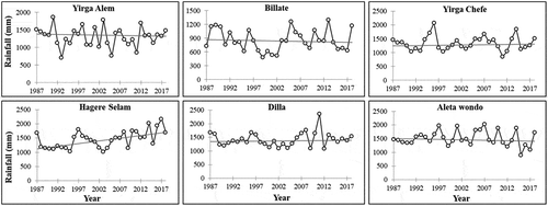
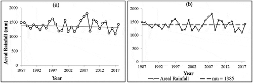
The basin-wide areal rainfall trend showed no significant change in annual rainfall in the Gidabo watershed (Fig. 5(a)), and this is in line with the study of Fenta et al. (2017). The Pettitt test results exhibit an abrupt change in annual rainfall at Hagere Selam station only (Fig. 4). The mean annual rainfall at Hagere Selam station reveals an upward shift in 2005. The remaining five stations did not show any significant change point in annual rainfall. Further, the Pettitt test could not detect any jump point in basin-wide areal rainfall (Fig. 5(b)). In general, no significantly increasing/decreasing trend in annual rainfall was observed in the study watershed. Hence, any change in the hydrological components during the study period (1988–2018) might be attributed to the effect of LULC changes.

Figure 4. Homogeneity test of the annual mean rainfall at six stations, where mu is the annual mean rainfall (mm), mu1 is the annual mean rainfall (mm) before the change point and mu2 is the annual mean rainfall (mm) after the change point

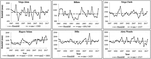
Figure 5. (a) Linear trend of annual mean areal rainfall and (b) Pettitt homogeneity tests of annual mean areal rainfall

5.2 Evaluation of LULC change and accuracy assessment

The Landsat satellite images, in combination with unsupervised and supervised classification techniques, were used to map the LULC in the study watershed in the years 1988, 2000 and 2018, and, subsequently, changes in the LULC characteristics were calculated. Around 150 or more reference ground truth locations were used to assess the accuracy of the classification. The error matrix (Table 4) obtained from the analysis reveals an overall accuracy of 85.34%, with a kappa statistic of 82.46% for the LULC map of 2018. Similarly, for the LULC maps for 1988 and 2000, overall accuracies of 81.21% and 85.16% and kappa statistics of 77.23% and 82.24%, respectively, were obtained. The discrimination of evergreen forest and agroforestry was found to be tedious and highly challenging during the classification process and may remain a source of uncertainty. However, the overall accuracy achieved met the minimum criteria for further analysis as suggested by Ariti et al. (2015).

Table 4. Error matrix for the 2018 classified map. CL: cultivation; EF: evergreen forest; AF: agroforestry; SH: shrubland; GL: grassland; UR: urban area; WR: water; WL: wetland

Classified data	Reference data
	CL	EF	AF	GL	SH	UR	WR	WL	Row total	User’s accuracy (%)
CL	36	1	2	5	0	2	0	0	46	78.26
EF	0	28	1	0	0	0	0	0	29	96.55
AF	2	5	37	0	0	1	0	0	45	82.22
GL	0	1	1	23	1	0	0	0	26	88.46
SH	0	0	0	1	13	0	0	0	14	92.86
UR	1	0	0	0	0	12	0	0	13	92.31
WR	0	0	0	0	0	0	5	1	6	83.33
WL	0	0	0	1	1	0	1	9	12	75.00
Column total	39	35	41	30	15	15	6	10	191
Producer’s accuracy (%)	92.31	80.00	90.24	76.67	86.67	80.00	83.33	90.00

The areal extent and rate of change of LULC in the Gidabo watershed are shown in Fig. 6 and presented in Table 5. Agroforestry, cultivated area, evergreen forest and grassland cover a significant portion of the study watershed over the entire study period horizon. An appraisal of LULC maps for the years 1988, 2000 and 2018 suggests that the most significant changes occurred in the cultivated area, agroforestry and evergreen forest classes during the study period from 1988 to 2018. The cultivated land increased from 19.62% to 33.36%, with a rate of change of 32.85 km²/year from 1988 to 2000, while the agroforestry, grassland and evergreen forest area decreased from 51.36% to 42.86%, 10.76% to 10.04% and 15.16% to 11.97%, respectively, with a rate of change of 20.33, 1.72 and 7.63 km²/year during the same period.

Figure 6. Areal extents of LULC types in the study area for the years 1988, 2000 and 2018

Note: CL: cultivation; FE: evergreen forest; AF: agroforestry; SH: shrubland; GL: grassland; UR: urban area; WR: water; WL: wetland.

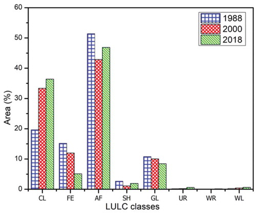
Table 5. Areal extents and rate of change of Gidabo basin land-use/land-change (LULC) classes. CL: cultivation; EF: evergreen forest; AF: agroforestry; SH: shrubland; GL: grassland; UR: urban area; WR: water; WL: wetland

LULC classes	Areal extent (%)			Rate of change (km^2/year)
	1988	2000	2018	2000–1988	2018–2000	2018–1988
CL	19.62	33.36	36.38	+32.85	+5.21	+16.80
EF	15.16	11.97	5.08	−7.63	−11.90	−10.11
AF	51.36	42.86	46.86	−20.33	+6.91	−4.51
SH	2.66	1.11	1.90	−3.72	+1.38	−0.76
GL	10.76	10.04	8.43	−1.72	−2.78	−2.34
UR	0.15	0.22	0.59	+0.17	+0.65	+0.45
WR	0.006	0.04	0.13	+0.07	+0.16	+0.12
WL	0.27	0.40	0.61	+0.30	+0.36	+0.34

After the year 2000, the areal extent of agroforestry and shrubland started to increase, from 42.86% to 46.86% and 1.11% to 1.90%, respectively, with respective rates of change of 6.9 and 1.38 km²/year. During this period, the expansion of cultivated land was gradual, from 33.36% to 36.38%, with a rate of change of 5.21 km²/year. On the other hand, evergreen forest and grassland cover decreased consistently from 2000 to 2018. These conditions occurred because of the growing population, which triggered the demand for new agricultural land and fuelwood, which in turn brought about the reduction in the other LULC classes (Ariti et al. 2015, Liyew et al. 2019a). Nonetheless, the increased agroforestry and gradual expansion of cultivated land over the period 2000–2018 demonstrates that the environment was recovering from the devastating drought and forest clearance for firewood and cultivation. During this period, the Ethiopian government introduced a plantation programme, and extensive soil and water conservation measures were carried out by the public (Ariti et al. 2015, Liyew et al. 2019a). Other authors have also observed increases in cultivated land at the expense of forest land, grassland and shrubland, such as Ariti et al. (2015) in the Central Rift Valley of Ethiopia; Gebremicael et al. (2013) and Ayele et al. (2017) in the Upper Blue Nile basin, Ethiopia; Gashaw et al. (2018) in the Andassa watershed, Blue Nile basin, Ethiopia; and Liyew et al. (2019a) in the Upper Blue Nile basin of northwestern Ethiopia.

5.3 Calibration and validation of the model

Table 6 shows the sensitivity analysis conducted for 14 hydrological parameters of the SWAT model affecting the surface runoff, lateral flow, groundwater flow and evapotranspiration in the study watershed. The initial values of these parameters were taken from the SWAT database and the literature. These parameters were calibrated using the observed flow values at Aposto and Measa gauging sites. The calibrated values for the 12 most sensitive parameters that influence the hydrological processes in the Gidabo watershed for the Aposto and Measa catchments are presented in Table 7.

Table 6. Sensitive parameters and their ranks at Measa gauge. The t statistic and p value (Abbaspour et al. 2007, Gashaw et al. 2018) were used to establish significance. SCS: Soil Conservation Service

Rank	Parameter	Descriptions	t	p
14	r__OV_N.hru	Manning’s “n” value for overland flow	−0.31	0.75
13	r__HRU_SLP.hru	Average slope steepness	0.37	0.71
12	v__REVAPMN.gw	Threshold depth of water in the shallow aquifer for “revap” to occur (mm)	0.51	0.61
11	v__ALPHA_BF.gw	Baseflow alpha factor	−0.51	0.60
10	r__SLSUBBSN.hru	Average slope length	0.62	0.53
9	r__SOL_AWC (.).sol	Available water capacity of the soil layer	1.63	0.103
8	r__SOL_Z(.).sol	Depth from the soil surface to the bottom of the layer	4.79	0.0022
7	v__GW_REVAP.gw	Revap coefficient	5.36	0.0012
6	r__SOL_K(.).sol	Saturated hydraulic conductivity (mm/h)	−7.25	0.0
5	v__RCHRG_DP.gw	Deep aquifer percolation fraction	−9.54	0.0
4	v__GWQMN.gw	Threshold depth of water in the shallow aquifer required for return flow to occur (mm)	10.06	0.0
3	v__ESCO.hru	Soil evaporation compensation coefficient	−11.23	0.0
2	v__CANMX.hru	Maximum canopy storage	11.45	0.0
1	r__CN2.mgt	SCS runoff curve number for moisture condition II	−37.34	0.0

v__ means the actual parameter value will be replaced by an optimized value, and r__ means the actual parameter value will be multiplied by [1+ the optimized value].

Table 7. Calibrated values of sensitive parameters for the Aposto and Measa gauging sites

Parameter	Ranges	Optimized parameter values
		Aposto	Measa
r__CN2.mgt	$\pm 0.2$	−0.108	−0.056
v__CANMX.hru	0–100	7.09	9.90
v__ESCO.hru	0–1	0.85	0.84
v__GWQMN.gw	0–5000	3690	3400
r__SOL_K.sol	$\pm 0.8$	−0.2	−0.388
v__RCHRG_DP.gw	0–1	0.591	0.13
r__SOL_Z.sol	$\pm 0.25$	0.21	0.0175
v__GW_REVAP.gw	0.02–0.2	0.076	0.079
r__SLSUBBSN.hru	0–0.2	0.161	0.1542
v__ALPHA_BF.gw	0–1	0.091	0.448
v__REVAPMN.gw	0–500	344.6	298.3
r__SOL_AWC.sol	$\pm 0.25$	−0.182	−0.137

Figures 7 and Figs 8 show the calibration and validation results of monthly runoff at Measa and Aposto gauging sites, respectively, indicating a good agreement between the simulated and observed hydrographs. The scatter plots (Figs 9 and Figs 10) also display a fair distribution of the observed and simulated streamflows in the calibration and validation stages for Measa and Aposto gauging sites, respectively. Furthermore, a good model performance was attained for both Measa and Aposto gauging sites (Table 8), with NSE > 0.65, R² > 0.70 and PBIAS < ±10 in calibration and validation. Based on the model performance, the calibrated SWAT model was used to assess the hydrological response to LULC changes in the Gidabo watershed.

Figure 7. Calibration and validation of simulated and observed monthly streamflow at Measa gauge

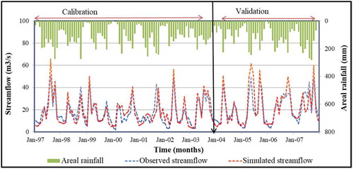
Figure 8. Calibration and validation of simulated and observed monthly streamflow at Aposto gauge

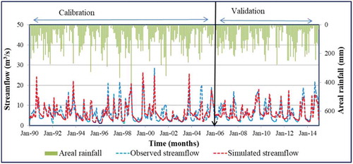
Figure 9. Scatter plots of measured and simulated data at Measa gauge during (a) calibration and (b) validation

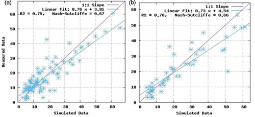
Figure 10. Scatter plots of measured and simulated data at Aposto gauge during (a) calibration and (b) validation

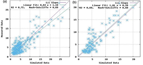
Table 8. Performance indices of the calibration and validation of the SWAT model. R²: coefficient of determination; NSE: Nash-Sutcliffe efficiency; PBIAS: percent bias

Stage	Gauge site	R^2	NSE	PBIAS
Calibration	Measa	0.75	0.67	−1.88
	Aposto	0.72	0.69	5.51
Validation	Measa	0.78	0.66	−7.29
	Aposto	0.69	0.68	4.97

5.4 Hydrological responses to LULC changes at the basin level

The yearly mean basin estimates of surface runoff, water yield, baseflow, lateral flow, percolation and ET and their relative changes at the basin outlet, which have been estimated from the 1988, 2000 and 2018 LULC maps, are shown in Table 9. Following an expansion in cultivated land and urban area and a reduction in evergreen forest, grassland and agroforestry, the yearly mean surface runoff showed a reliably increasing pattern, from 151.4 mm in 1988 to 173.1 mm in 2000 and 175.0 mm in 2018 (Table 9). Compared with the period of 2000 and 2018 (1.10%), the yearly mean surface runoff between 1988 and 2000 (14.33%) is higher. This is due to the drastic expansion of cultivated land between 1988 and 2000. In contrast, the baseflow, lateral flow and percolation showed a decreasing trend, from 89.0 to 79.9 mm, 69.2 to 65.0 mm and 287.9 to 277.7 mm, respectively, between 1988 and 2018 (Table 9). However, the changes in water yield and ET were inconsistent. For instance, the estimated annual average ET decreased from 880.5 mm to 863.4 mm (by 1.94%) between 1988 and 2000. This decrease was mainly caused by the contraction of evergreen forest, agroforestry, grassland and shrubland and the drastic expansion of cultivated land between 1988 and 2000. In contrast, the annual average ET increased from 863.4 to 868.3 mm (by 0.57%) between 2000 and 2018 (Table 9), as a result of the increase in agroforestry through replantation activity and the gradual expansion of cultivated land. The water yield increased from 306.6 to 324.9 mm between 1988 and 2000 and then diminished to 319.9 mm in 2018. The water yield in 2018 was less than that in 2000, as it is mainly the summation of surface runoff, lateral flow and baseflow. Thus, the decrease in baseflow and lateral flow and the slight increase of surface runoff in 2018 reduced the total upsurge in water yield.

Table 9. Annual mean hydrological components (1988–2018) during the different periods of the LULC study

Hydrological component (mm)	Study period			Relative change (%)
	1988	2000	2018	1988–2000	2000–2018	1988–2018
Surface runoff	151.4	173.1	175.0	14.33	1.10	15.6
Lateral flow	69.2	67.7	65.0	−2.17	−4.00	−6.07
baseflow	89.0	84.1	79.9	−5.5	−4.99	−10.22
Water yield	306.6	324.9	319.9	5.97	−1.54	4.34
Evapotranspiration	880.5	863.4	868.3	−1.94	0.57	−1.38
Percolation	287.9	281.8	277.7	−2.12	−1.42	−3.54

The results for baseflow, lateral flow and percolation (Table 9) show a reduction throughout the study period. This is because the depletion in vegetation cover added to the low penetration and canopy interception, so that the incoming rainfall was converted to surface runoff (Nie et al. 2011, Ayele et al. 2017, Liyew et al. 2019b). On the other hand, the transition of evergreen forest and grassland to cultivated and urban areas resulted in increases in impervious surface cover (Gyamfi et al. 2016). Also, on cultivated land, the soil particles are easily detached by the impact of rainfall. Consequently, upper layers of the pores are clogged, which leads to a reduction in the infiltration rate. As a result, a consistent increase in surface runoff was observed (Table 9).

The results of this study are in agreement with other research studies within the Andassa watershed, Blue Nile Basin, Ethiopia (Gashaw et al. 2018), and inside the Upper Blue Nile Basin, Ethiopia (Ayele et al. 2017), which found that cultivated land is expanding at the cost of vegetation cover. As a result, surface runoff is enhanced and baseflow diminished. Nie et al. (2011) and Gyamfi et al. (2016) also ascribed the overall escalation of surface runoff to the growth of urban area and cultivated land and the shrinking of vegetation cover.

5.5 Response of hydrological components to LULC changes at the sub-basin level

The spatial distributions of the changes of major LULC classes and the yearly mean hydrological components between 1988 and 2018 are shown in Figs 11 and Figs 12, respectively. Changes in land use mainly occurred in the central and southern parts of the basin (Fig. 11). Cultivated land is mainly expanded to the southern and northeastern parts of the basin at the expense of evergreen forest, agroforestry and grassland. The most significant increase in surface runoff and decrease in groundwater flow also mainly occurred in the central and southern parts of the basin (Fig. 12). The average annual surface runoff in all sub-basins was increased by 28.61 mm. Surface runoff changes in the basins increased in almost all sub-basins, especially in the central and downstream parts of the basin following the conversion of evergreen forest, agroforestry and grassland to cultivated and urban areas. Nevertheless, a decrease in surface runoff has also occurred in the northwestern part of the basin, related to the increase in agroforestry. The spatial distribution of water yield showed a similar trend to the surface runoff.

Figure 11. Spatial distribution of changes in LULC classes at the sub-basin level for the period 1988–2018

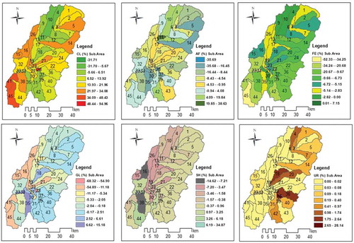
Figure 12. Spatial distribution of changes in the hydrological components at the sub-basin level for the period 1988–2018

Note: SURQ: surface runoff; WYLD: water yield; GWQ: baseflow; LATQ: lateral flow; PERC: percolation; ET: evapotranspiration.

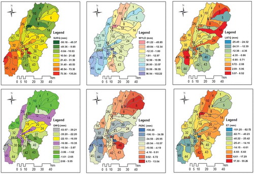
The baseflow in 45 sub-basins demonstrated a decreasing pattern during 1988 and 2018, with the most significant reduction occurring in the southern and central parts of the basin. Meanwhile, the yearly average ET in all sub-basins decreased by 15.13 mm, with the most extreme decrease in the southern part of the basin (Fig. 12). However, in certain parts of the basin, ET increased by a maximum of 55.26 mm at sub-basin 6. Generally, ET decreased in the southern and southeastern parts of the basin. The resilient nature of cultivated and urban areas reveals a decline in the recharge rate, which was revealed by the spatial trend of percolation in many sub-basins. Sub-basins that have experienced a more significant increase in cultivated and urban areas generate more surface runoff and water yield in contrast to other hydrological components. Marhaento et al. (2017) argue that the impact of land-use changes on the water budget elements vary among sub‐basins depending on the scale of changes in LULC classes.

The sub-basin-level (Fig. 12) impacts of LULC change on hydrological elements were greater than those at the level of the basin as a whole (Table 9). Hence, more articulated changes of hydrological components were observed at the sub-basin level because of the uneven spatial distribution of LULC alterations. The impacts of LULC changes were greater at a smaller scale. However, the responses of hydrological elements to LULC changes were relatively small at the watershed level due to compensating effects (Gebremicael et al. 2019). Mwangi et al. (2016) also concluded that the impact of agroforestry was greater at a scale smaller than the entire watershed.

5.6 Influence of individual LULC changes on changes in hydrological components

A Pearson matrix of six LULC classes and six hydrological components is shown in Table 10. The results reveal that nearly all LULC classes have a fair association with various hydrological components. Correspondingly, appropriate correlations among the hydrological components are additionally observed. As an example, cultivated land had a positive correlation with surface runoff (0.82) and water yield (0.90), while its correlation with baseflow, lateral flow, percolation and ET is negative (Table 10). The regression coefficients (Table 11) additionally confirm that cultivated land influences surface runoff and water yield positively. However, its influence on baseflow, lateral flow, percolation and ET is negative. Likewise, the correlation between surface runoff and water yield is positive, but it is negative between surface runoff, water yield and base flow, lateral flow, percolation and ET (Table 10). Further, the VIP values (Fig. 14) show that cultivated land is an essential factor for surface runoff, lateral flow and ET.

Table 10. Pearson correlation matrix for changes in LULC and hydrological components between 1988 and 2018. CL: cultivation; EF: evergreen forest; AF: agroforestry; GL: grassland; SH: shrubland; UR: urban area; SURQ: surface runoff; WYLD: water yield; GWQ: baseflow; LATQ: lateral flow; PERC: percolation; ET: evapotranspiration. Values in bold are different from 0 with a significance level of α = 0.05. This is confirmed by the table of p values (p < 0.0001)

Variables	CL	EF	AF	GL	SH	UR	SURQ	WYLD	GWQ	LATQ	PERC	ET
CL	1.00
EF	−0.21	1.00
AF	−0.54	−0.03	1.00
GL	−0.76	−0.04	0.01	1.00
SH	−0.28	−0.63	0.02	0.39	1.00
UR	−0.13	0.07	−0.23	0.10	0.01	1.00
SURQ	0.82	−0.33	−0.67	−0.47	−0.10	0.25	1.00
WYLD	0.90	−0.20	−0.69	−0.57	−0.23	0.11	0.95	1.00
GWQ	−0.09	0.49	0.31	−0.21	−0.26	−0.48	−0.52	−0.29	1.00
LATQ	−0.44	0.09	0.09	0.50	0.06	0.00	−0.38	−0.36	−0.24	1.00
PERC	−0.02	0.38	0.29	−0.21	−0.19	−0.67	−0.48	−0.25	0.96	−0.22	1.00
ET	−0.92	0.15	0.64	0.62	0.24	0.12	−0.87	−0.96	0.09	0.40	0.00	1.00

Table 11. Results of partial least squares regression (PLSR). Positive and negative signs show the position of influence. CL: cultivation; EF: evergreen forest; AF: agroforestry; GL: grassland; SH: shrubland; UR: urban area; SURQ: surface runoff; WYLD: water yield; GWQ: baseflow; LATQ: lateral flow; PERC: percolation; ET: evapotranspiration

PLSR model	Response variable	PLSR predictors
		CL	EF	AF	GL	SH	UR
PLSR1	SURQ	0.69	−0.87	−1.17	−0.44	−0.02	1.91
	WYLD	0.58	−0.47	−0.86	−0.50	−0.32	0.96
PLSR2	GWQ	−0.02	0.36	0.21	−0.13	−0.34	−1.37
	PERC	−0.04	0.58	0.34	−0.21	−0.56	−2.23
PLSR3	LATQ	−0.06	0.03	0.02	0.11	0.03	0.00
PLSR4	ET	−0.58	0.20	0.71	0.61	0.58	0.46

Grassland is seen to have an excellent association with surface runoff, water yield, lateral flow and ET, with correlation coefficients of −0.47, −0.57, +0.50 and +0.62, respectively. In contrast, grassland has a relatively low correlation with baseflow (−0.21) and percolation (−0.21). The regression coefficient (Table 11) also attests that grassland influences lateral flow and ET positively and surface runoff and water yield negatively. The positive impact of grassland on lateral flow and ET is due to a shallow vertical root system, which enables the grasses to use water in the shallow soil that facilitates lateral flow and ET (Gyamfi et al. 2016). VIP values also confirm the grassland to be most impactful factor for lateral flow and ET (Fig. 14).

Evergreen forest shows a high correlation with surface runoff, baseflow and percolation, with correlation coefficients of −0.33, +0.49 and +0.38, respectively. In contrast, evergreen forest shows a relatively low correlation with other hydrological components (Table 10). This is also attested by the regression coefficient (Table 11); surface runoff is influenced negatively, and baseflow positively, by evergreen forest. VIP values too confirm that evergreen forest is an essential contributor to baseflow and percolation. The correlation matrix reveals that the agroforestry is highly associated with surface runoff (−0.67), water yield (−0.69), baseflow (+0.31) and ET (0.64). The image of the correlation matrix (Fig. 13) provides a pictorial representation of the relationship between LULC classes and hydrological components.

Figure 13. Image of PLSR correlation matrixes

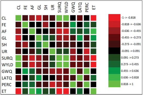
Figure 14. Variable importance of project (VIP) values at the 95% significance level for the six land-use/land-cover (LULC) classes for hydrological components

Note: VIP > 0.8 indicates the most relevant LULC classes to explain hydrological components; the horizontal dashed lines show VIP > 1 and VIP > 0.8.

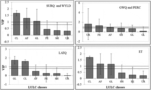
In general, the surface runoff and water yield are profoundly related to change in the cultivated and urban areas. In contrast, baseflow, lateral flow, percolation and ET are negatively related to change in cultivated and urban areas. Moreover, baseflow, lateral flow, percolation and ET are highly positively related to alteration of evergreen forest, agroforestry and grassland, while surface runoff inversely correlates to alteration in these areas. The shrubland LULC classes also show a positive or negative impact on all hydrological components (Table 11) although these effects are not statistically significant (Table 10), perhaps because of the issue of multicollinearity.

6 Conclusions

In this study, an attempt is made to assess the hydrological responses to LULC changes using the SWAT model and statistical analysis. The following conclusions can be derived from the study:

1. The MK test showed no significant trend in basin-wide annual rainfall during the study period (1988–2018) at the 95% significance level. The Pettitt test too could not detect any break in the basin-wide annual rainfall. Hence, any change in hydrological components during the study period (1988–2018) might be attributable to the effects of LULC changes.

2. An assessment of LULC maps for 1988, 2000 and 2018 suggests that the most sizable changes happened in cultivated land, agroforestry, evergreen forest, grassland and urban areas. The study shows an increase in cultivated and urban areas and a decline in evergreen forest, agroforestry and grassland over the 31 years between 1988 and 2018. However, the increased agroforestry and gradual expansion of cultivated land over the period 2000–2018 confirmed that the environment was recovering from land devastated by drought and wooded areas cleared for firewood and cultivation.

3. Following an increase in cultivated and urban areas and a decline in evergreen forest, agroforestry, grassland and shrubland, the annual mean surface runoff demonstrated a persistently increasing trend, from 151.4 mm in 1988 to 173.1 mm in 2000 and 175.0 mm in 2018. In contrast, baseflow, percolation and ET showed declining trends. More noticeable changes in hydrological components were observed at the sub-basin scale, mainly associated with the uneven spatial distribution of LULC changes.

4. The Pearson correlation matrix confirmed that nearly all LULC classes have a good relationship with various hydrological components. PLSR analysis revealed that cultivated, agroforestry, grassland, evergreen forest and urban areas are the most applicable variables to explain surface runoff, water yield, baseflow and percolation for Gidabo basin. Likewise, lateral flow and ET were highly influenced by cultivated land, agroforestry and grassland.

5. This study has attributed contributions of LULC changes to hydrological components, providing visible information that will allow stakeholders and decision-makers to make important decisions regarding soil and water conservation measures and optimum allocation of water resources. However, change in LULC is expected to continue into the near future, and it will be crucial to examine its impact on future basin hydrology for planning future water management strategies. We also recommend further studies of the future climate change effects on the components of the water budget of Gidabo watershed.

Acknowledgements

The authors express their thanks to the National Meteorological Agency of Ethiopia (NMAoE) and the Ministry of Water, Irrigation and Electricity of Ethiopia (MoWIE) for providing the climate and hydrological data respectively. The authors are also thankful to the United States Geological Survey (USGS) for the Landsat images and DEM data. The authors are very thankful to the Indian Institute of Technology Roorkee, Institute of Computer Center for providing the ERDAS 2018 and ArcGIS 10.5 software packages.

Disclosure statement

No potential conflict of interest was reported by the authors.

References

- Abbaspour, K.C., Vaghefi, S.A., and Srinivasan, R., 2017. A guideline for successful calibration and uncertainty analysis for soil and water assessment: a review of papers from the 2016 international SWAT conference. Water, 10 (1), 6.
- Abbaspour, K.C., et al., 2007. Modelling hydrology and water quality in the pre-alpine/alpine Thur watershed using SWAT. Journal of Hydrology, 333 (2–4), 413–430. doi:10.1016/j.jhydrol.2006.09.014
- Abdi, H., 2007. Partial least‐square regression. In: N. Salkind, ed. Encyclopedia of measurement and statistics. Thousand Oaks (CA): Sage, 1–13.
- Abdi, H., 2010. Partial least squares regression and projection on latent structure regression (PLS regression). WIREs Computational Statistics, 2 (1), 97–106. doi:10.1002/wics.51
- Ariti, A.T., van Vliet, J., and Verburg, P.H., 2015. Land-use and land-cover changes in the Central Rift Valley of Ethiopia: assessment of perception and adaptation of stakeholders. Applied Geography, 65, 28–37. doi:10.1016/j.apgeog.2015.10.002
- Arnold, J.G., et al., 1998. Large area hydrologic modeling and assessment part I: model development. Journal of the American Water Resources Association, 34 (1), 73–89. doi:10.1111/j.1752-1688.1998.tb05961.x
- Ayele, T., et al., 2017. Hydrological responses to land use/cover changes in the source region of the Upper Blue Nile basin, Ethiopia. Science of the Total Environment, 575, 724–741. doi:10.1016/j.scitotenv.2016.09.124
- Baker, T.J. and Miller, S.N., 2013. Using the soil and water assessment tool (SWAT) to assess land use impact on water resources in an East African watershed. Journal of Hydrology, 486, 100–111. doi:10.1016/j.jhydrol.2013.01.041
- Belihu, M., et al., 2018. Hydro-meteorological trends in the Gidabo catchment of the Rift Valley Lakes basin of Ethiopia. Physics and Chemistry of the Earth, 104, 84–101. doi:10.1016/j.pce.2017.10.002
- Brito, R.S., Almeida, M.C., and Matos, S.J., 2017. Estimating flow data in urban drainage using partial least squares regression. Urban Water Journal, 14 (5), 467–474. doi:10.1080/1573062X.2016.1177099
- Carrascal, L.M., Galván, I., and Gordo, O., 2009. Partial least squares regression as an alternative to current regression methods used in ecology. Oikos, 118 (5), 681–690. doi:10.1111/j.1600-0706.2008.16881.x
- Chow, V.T., Maidment, D.R., and Mays, L.W., 1988. Applied hydrology. New York: McGraw-Hill.
- Fang, N., et al., 2015. Partial least squares regression for determining the control factors for runoff and suspended sediment yield during rainfall events. Water, 7 (12), 3925–3942. doi:10.3390/w7073925
- Fenta, A.A., et al., 2017. Spatial distribution and temporal trends of rainfall and erosivity in the Eastern Africa region. Hydrological Processes, 31 (25), 4555–4567. doi:10.1002/hyp.11378
- Garg, V., et al., 2019. Human-induced land use land cover change and its impact on hydrology. HydroResearch, 1, 48–56. doi:10.1016/j.hydres.2019.06.001
- Gashaw, T., et al., 2017. Evaluation and prediction of land use/land cover changes in the Andassa watershed, Blue Nile basin, Ethiopia. Environmental Systems Research, 6 (1), 17. doi:10.1186/s40068-017-0094-5
- Gashaw, T., et al., 2018. Modeling the hydrological impacts of land use/land cover changes in the Andassa watershed, Blue Nile basin, Ethiopia. Science of the Total Environment, 619–620, 1394–1408. doi:10.1016/j.scitotenv.2017.11.191
- Gebremicael, T.G., et al., 2013. Trend analysis of runoff and sediment fluxes in the Upper Blue Nile basin: a combined analysis of statistical tests, physically-based models and landuse maps. Journal of Hydrology, 482, 57–68. doi:10.1016/j.jhydrol.2012.12.023
- Gebremicael, T.G., Mohamed, Y.A., and Van Der Zaag, P., 2019. Attributing the hydrological impact of different land use types and their long-term dynamics through combining parsimonious hydrological modelling, alteration analysis and PLSR analysis. Science of the Total Environment, 660, 1155–1167. doi:10.1016/j.scitotenv.2019.01.085
- Godoy, J.L., Vega, J.R., and Marchetti, J.L., 2014. Chemometrics and intelligent laboratory systems relationships between PCA and PLS-regression. Chemometrics and Intelligent Laboratory Systems, 130, 182–191. doi:10.1016/j.chemolab.2013.11.008
- Gyamfi, C., Ndambuki, J.M., and Salim, R.W., 2016. Hydrological responses to land use/cover changes in the Olifants basin, South Africa. Water, 8 (12), 588.
- Kendall, M.G., 1975. Rank correlation methods. London: Charles Griffin.
- Legesse, D., Vallet-Coulomb, C., and Gasse, F., 2003. Hydrological response of a catchment to climate and land use changes in Tropical Africa: case study south central Ethiopia. Journal of Hydrology, 275 (1–2), 67–85. doi:10.1016/S0022-1694(03)00019-2
- Liyew, M., Tsunekawa, A., and Haregeweyn, N., 2019a. Exploring land use/land cover changes, drivers and their implications in contrasting agro-ecological environments of Ethiopia. Land Use Policy, 87, 104052. doi:10.1016/j.landusepol.2019.104052
- Liyew, M., et al., 2019b. Hydrological responses to land use/land cover change and climate variability in contrasting agro-ecological environments of the Upper Blue Nile basin, Ethiopia. Science of the Total Environment, 689, 347–365. doi:10.1016/j.scitotenv.2019.06.338
- Mankin, K.R.D., et al., 2010. Modeling nutrient runoff yields from combined in-field crop management practices using SWAT. American Society of Agricultural and Biological Engineers, 53 (5), 1557–1568.
- Mann, H.B., 1945. Nonparametric tests against trend. The Econometric Society, 13 (3), 245–259. doi:10.2307/1907187
- Marhaento, H., et al., 2017. Attribution of changes in the water balance of a tropical catchment to land use change using the SWAT model. Hydrological Processes, 31 (11), 2029–2040. doi:10.1002/hyp.11167
- Mechal, A., Wagner, T., and Birk, S., 2015. Recharge variability and sensitivity to climate: the example of Gidabo River basin, Main Ethiopian Rift. Journal of Hydrology: Regional Studies, 4, 644–660.
- Mevik, B.H. and Wehrens, R., 2007. The pls package: principal component and partial least squares regression in R. Journal of Statistical Software, 18 (2), 2. doi:10.18637/jss.v018.i02
- Monteith, J.L., 1965. Evaporation and environment.Symposia of the Society for Experimental Biology, 19 (2393175), 205–234.
- Moriasi, D.N., et al., 2007. Model evaluation guidelines for systematic quantification of accuracy in watershed simulations. American Society of Agricultural and Biological Engineers, 50 (3), 885–900.
- Mwangi, H.M., et al., 2016. Modelling the impact of agroforestry on hydrology of Mara River basin in East Africa. Hydrological Processes, 30 (18), 3139–3155. doi:10.1002/hyp.10852
- Neitsch, S.L., et al., 2011. Soil and water assessment tool theoretical documentation version 2009. Texas Water Resources Institute.
- Nie, W., et al., 2011. Assessing impacts of Landuse and Landcover changes on hydrology for the upper San Pedro watershed. Journal of Hydrology, 407 (1–4), 105–114. doi:10.1016/j.jhydrol.2011.07.012
- Niraula, R., Meixner, T., and Norman, L.M., 2015. Determining the importance of model calibration for forecasting absolute/relative changes in streamflow from LULC and climate changes. Journal of Hydrology, 522, 439–451. doi:10.1016/j.jhydrol.2015.01.007
- Pettitt, A.N., 1979. A non-parametric approach to the change-point problem. Applied Statistics, 28 (2), 126–135. doi:10.2307/2346729
- Schilling, K.E., et al., 2014. The potential for agricultural land use change to reduce flood risk in a large watershed. Hydrological Processes, 28 (8), 3314–3325. doi:10.1002/hyp.9865
- Setegn, S.G., et al., 2009. Spatial delineation of soil erosion vulnerability in the Lake Tana basin, Ethiopia. Hydrol. Process., 3750, 3738–3750.
- Shawul, A.A., Chakma, S., and Melesse, A.M., 2019. The response of water balance components to land cover change based on hydrologic modeling and partial least squares regression (PLSR) analysis in the Upper Awash basin. Journal of Hydrology: Regional Studies, 26, 100640.
- Shi, Z.H., et al., 2013. Partial least-squares regression for linking land-cover patterns to soil erosion and sediment yield in watersheds. Journal of Hydrology, 498, 165–176. doi:10.1016/j.jhydrol.2013.06.031
- Tekleab, S., Mohamed, Y., and Uhlenbrook, S., 2013. Hydro-climatic trends in the Abay/Upper Blue Nile basin, Ethiopia. Physics and Chemistry of the Earth, 61–62, 32–42. doi:10.1016/j.pce.2013.04.017
- USDA-SCS (US Department of Agriculture Soil Conservation Service), 1972. National engineering handbook,section 4: hydrology. Washington, DC: US Department of Agriculture Soil Conservation Service.
- Wagner, P.D., Kumar, S., and Schneider, K., 2013. An assessment of land use change impacts on the water resources of the Mula and Mutha Rivers catchment upstream of Pune, India. Hydrology and Earth System Sciences, 17 (6), 2233–2246. doi:10.5194/hess-17-2233-2013
- Wold, S., Sjostrom, M., and Eriksson, L., 2001. PLS-regression: a basic tool of chemometrics. Chemometrics and Intelligent Laboratory Systems, 58 (2), 109–130.
- WWDSE (Water Works Design and Supervision Enterprise), 2007. Study and design of Gidabo irrigation project, final feasibility report. Addis Ababa, Ethiopia: Water Works Design and Supervision Enterprise.
- Yan, B., et al., 2013. Impacts of land use change on watershed streamflow and sediment yield: an assessment using hydrologic modelling and partial least squares regression. Journal of Hydrology, 484, 26–37. doi:10.1016/j.jhydrol.2013.01.008
- Yan, R., et al., 2018. Spatial patterns of hydrological responses to land use/cover change in a catchment on the Loess Plateau, China. Ecological Indicators, 92, 151–160. doi:10.1016/j.ecolind.2017.04.013
- Zhang, L., et al., 2016. Hydrological impacts of land use change and climate variability in the headwater region of the Heihe River basin, Northwest China. PLoS ONE, 11, 6.
- Zhou, F., et al., 2013. Hydrological response to urbanization at different spatio-temporal scales simulated by coupling of CLUE-S and the SWAT model in the Yangtze River Delta region. Journal of Hydrology, 485, 113–125. doi:10.1016/j.jhydrol.2012.12.040