Scaling lognormal water retention curves for dissimilar soils

ABSTRACT

The main objective of the present research is scaling lognormal water retention curves for dissimilar soils. This method requires a reference curve and the amount of water content in a particular suction. The scaling factor in this method equals the log amount of moisture in a particular suction (e.g. $S{e}_{5000}$) in the reference soil to the log amount of water content in the same suction in the soil. The proposed method was evaluated for 14 different soil samples. The scaling factor obtained by this method was evaluated by the scaling factor obtained from the optimization method (${\alpha }_{Opt}$). The results showed that the average scaling factor based on $S{e}_{5000}$ is closest to the average ${\alpha }_{Opt}$ . The water retention curve obtained by the method presented in this research is fitted on the water retention curve obtained from the lognormal model with superior accuracy.

KEYWORDS:

• water retention curve
• scaling
• similar media

Editor A. Fiori Associate Editor P. van Oel

1 Introduction

Determining the soil water retention curve (SWRC), which represents the relationship between water pressure and water content, is essential for the study of water flow and chemical transfer in an unsaturated medium (Pollacco et al. 2017). On the other hand, changes in soil texture, soil pH, cation exchange capacity, organic matter, and the thickness of clay particles cause changes in the water–soil characteristic curve and therefore should be re-measured, which requires a significant investment of time and money. As a result, one of the major problems facing soil scientists is how to deal with soil variability. This variability, especially in soil hydraulic functions, including the moisture curve and the hydraulic conductivity function, makes it difficult to analyze water flow relationships in soil (Nasta et al. 2013, Ahmadi et al. 2014).

In recent years, researchers have come up with ways to obviate the need to measure farm data needed to express soil dynamics. One of these methods is scaling, which was first developed by Miller and Miller (1956) based on a similar media theory in water and soil science (Miller and Miller 1956, Sadeghi et al. 2016) and subsequently used extensively to evaluate the infiltration process (Sharma et al. 1980, Khatri and Smith 2006, Babaei et al. 2018, Chari et al. 2020), the hydraulic properties of soils (Ahuja and Williams 1991, Vogel et al. 1991, Kosugi and Hopmans 1998, Tuli et al. 2001, Nasta et al. 2013), soil variability (Warrick and Nielsen 1980), and general solutions to soil water movement equations (Sadeghi et al. 2012, Chari et al. 2019).

There are two common ways to obtain a scaling factor to scale an SWRC (Tillotson and Nielsen 1984): (1) a dimensional analysis technique, which is based on the existence of physical similarities in the system, such as similar media Miller and Miller (1956) and fractal dimension-based methods (Tyler and Wheatcraft 1990, Rieu and Sposito 1991); (2) the experimental method – so-called functional normalization – which is based on regression analysis.

In the first method, the scaling factor usually has a physical meaning. The studies of Kosugi and Hopmans (1998), Tuli et al. (2001), Meskini-Vishkaee et al. (2014), and Nasta et al. (2009) are examples of the application of the first method in soil hydraulic functions. Miller and Miller (1956) hypothesized that the microscopic structure of two soils that are geometrically similar differs only in proportions of a physical characteristic length. According to this theory, the hydraulic functions of different soils can be applied to a reference curve with ratios of a physical characteristic length.

Kosugi and Hopmans (1998) defined the microscopic resemblance of soils in a more tangible way than Miller and Miller. They hypothesized that the size of the soil pores followed a lognormal distribution and used the radius of the mid-sized soil pores as a physical feature length. Tuli et al. (2001), following Kosugi and Hopmans (1998), proposed a method for simultaneous scaling of SWRC and unsaturated hydraulic conductivity. Das et al. (2005) found that soil grouping using soil texture criteria was not sufficient to meet the geometric similarity criterion, and suggested that using the standard deviation of the pore-size distribution in a similar way improves scaling results. Sadeghi et al. (2016) showed that similarity (standard deviation of the pore size distribution) is not the only necessary condition for the validity of the Miller-Miller theory and defined a dimensionless parameter called “joint scaling factor.” They then evaluated their proposed method for six classes of similar soils.

Nasta et al. (2009) presented a scaling method based on a physical concept to express the variability of the water retention curve. To do this, they combined the scale method with particle size distribution and predicted the SWRC using minimal data. A comparison of the methods presented by Nasta et al. (2009) and Kosugi and Hopmans (1998) shows that Nasta et al.’s (2009) method predicts the water retention curve with greater accuracy. Meskini-Vishkaee et al. (2014) used particle size distribution and porosity to provide a physical method for scaling the water retention curve. The results showed that using this method, a water retention curve can be predicted with appropriate accuracy. It should be noted that in order to obtain the water retention curve using this method, it is necessary to know the particle size distribution and soil porosity.

Given that field soils are generally dissimilar, experimental hypotheses and the application of regression methods have been further expanded. In most of these methods, the optimal scaling factor is obtained by minimizing the square root difference between the average (reference) water retention curve and the measured water retention curve. Warrick et al. (1977) stated that a search for the length of a physical characteristic is not required to find scaling factors. They suggested that the reference curve can be determined by averaging all the curves, and then the scaling factors can be experimentally obtained in such a way that any scale curved with the least error occurs on the reference curve. Simmons et al. (1979) proposed a method for soil scaling by replacing the condition of similarity in the form of hydraulic functions with the geometric similarity of soils in Miller and Miller’s theory. Vogel et al. (1991) considered the linear variability of soils a necessary condition for scaling.

Hendrayanto et al. (2000) applied the functional normalization method to simultaneously scale the water retention curve and the unsaturated hydraulic conductivity of the soil. In this study, the scaling factor of the water retention curve and unsaturated hydraulic conductivity were obtained using optimization method and then, by combining these two methods, a factor for both was introduced. Ahuja and Williams (1991) converted the water retention curve presented by Gregson et al. (1987) to a linear state and expressed the relationship between the parameters of this model using the scaling process. Williams and Ahuja (2003) showed that the water retention curve obtained using the Brooks-Corey model (1964) can be scaled using the average mass distribution of particle size (λ), and a scaled equation is an expression parameter. All parameters of the Brooks-Cory model depend on the average particle size distribution (λ). Kozak and Ahuja (2005) used the particle size distribution parameter (λ) to scale penetration and redistribution.

One of the problems with these methods is to determine the average particle size distribution (λ); to do so, the available suction-moisture data must be obtained or calculated using transfer functions, which in turn causes errors. The application of the Kosugi and Hopmans method (1998), similarly to the previous methods, is limited to similar soils, which is a constraint on the scaling of real non-similar soils. Therefore, the main objective of this research is to provide a simple way to scale the water retention curve using the minimum field information (a reference water retention curve and the amount of moisture in a particular suction) so that it can be used for different soils. Also, the method presented in this study is compared with that of Kosugi and Hopmans (1998).

2 Materials and methods

2.1 Scaling

Based on the similar media theory of Miller and Miller (1956) and relying on the capillary and porous relationships in which suction (h) and unsaturated hydraulic conductivity (K) are inversely proportional to the inverse and square radii of the pores, respectively, it was expected that h and k would be mixed in different soils with a series of scaling factors. h and k in different soils can be scaled as follows:

(1) ${\alpha }_1{h}_1\left(S_e\right)={\alpha }_2{h}_2\left(S_e\right)=\dots ={\alpha }_i{h}_i\left(S_e\right)=h^{\ast }\left(S_e\right)$(1)

(2) $\frac{K_1\left(S_e\right)}{{\alpha }_1^2}=\frac{K_2\left(S_e\right)}{{\alpha }_2^2}=\dots =\frac{K_i\left(S_e\right)}{{\alpha }_i^2}=K^{\ast }\left(S_e\right)$(2)

where i represents the different soils; h* and K* are the scales of suction and hydraulic conductivity, respectively; and $S_e$is the effective saturation, defined as follows:

(3) $S_e=\frac{\theta -{\theta }_r}{{\theta }_s-{\theta }_r}$(3)

where θ is the volumetric water content, and ${\theta }_r$ and ${\theta }_s$ are the residual and saturated volumetric water content, respectively.

In order to scale based on physical concepts, Kosugi and Hopmans (1998) revisited the similar media theory of Miller and Miller (1956). But this time they described the microscopic resemblance of soils in a more tangible way than Miller and Miller. They assumed that the size of the soil pores would follow a lognormal distribution. Assuming the Kosugi lognormal model can be used for retention and hydraulic conductivity functions, then:

(4) $S_e=0.5erfc\frac{\mathrm{l}\mathrm{n}\left(h/h_{mi}\right)}{\sigma \sqrt{2}}$(4)

(5) $K_r=\frac{K}{K_s}=$(5)

where $erfc$ is a complementary error function, $h_{mi}$ is the median pressure head in each soil (suction in Se = 0.5), σ is the standard deviation of the log-transformed pore size, and $K_r$ is the relative hydraulic conductivity.

The reference curve parameters can be obtained using the arithmetic mean of the parameters of each soil as follows (Kosugi and Hopmans 1998, Tuli et al. 2001):

(6) ${\bar{h}}_m=exp\left[\left(1/I\right)\sum _{i=1}^{I}ln{h}_{m_i}\right]$(6)

(7) $\bar{\sigma }={\left[\left(1/I\right)\sum _{i=1}^I{\sigma }_i^2\right]}^{0.5}$(7)

where i and ־ denote individual soil and reference soil parameters, respectively.

2.2 The proposed method

The basic premise of the proposed method is that the shape of the water retention curve and the shape of the hydraulic conductivity curve have been almost constant despite the variation in the water content. The data required to obtain the specifications of the water retention curve for each soil using the scaling process to a reference infiltration curve, whose parameters are known, and a point of suction-moisture data are reduced. In this method, firstly the logarithm of the effective saturation value ($S_e$) is taken to get it out of the sigmoid function and turn it into an almost linear shape. Vogel et al. (1991) stated that the necessary condition for scale is the linear variability of soils. If the logarithm is taken on both sides of Equation (4)(4) $S_e=0.5erfc\frac{\mathrm{l}\mathrm{n}\left(h/h_{mi}\right)}{\sigma \sqrt{2}}$(4) , we have:

(8) $ln\left(S_e\right)=\mathrm{l}\mathrm{n}\left(0.5erfc\frac{\mathrm{l}\mathrm{n}\left(h/h_{mi}\right)}{\sigma \sqrt{2}}\right)$(8)

If the water content in a particular suction ($hi$) for each soil is known, then the scaling factor for each soil (${\alpha }_j$) is equal to:

(9) ${\alpha }_i={\left(\frac{\mathrm{l}\mathrm{n}\left(S_{e_i}\right)}{\mathrm{l}\mathrm{n}\left(S_{e_{ref}}\right)}\right)}_{hi}$(9)

where i is the soil number, $hi$ is the specific suction value (e.g. 330, 500, 1000 or …), and ${S_e}_{ref}$ is the relative saturation in the reference soil.

Then, the water retention curve for each soil is:

(10) $S_{e_{ij}}^{\ast }=exp\left[\frac{\mathrm{l}\mathrm{n}\left(S_{e_{ij}}\right)}{{\alpha }_i}\right]$(10)

where $S_{e_{ij}}^{\ast }$ represents the relative saturation scale value for different soils and suctions.

We can de-scale the water retention curve and obtain the water retention curve in real mode using the reference curve for each soil as follows:

(11) $S_{e_{ji}}=exp\left[{\alpha }_{i}ln{\left(S_{e_r}\right)}_j\right]$(11)

2.3 Optimization methods

The scaling factor can also be obtained by using the statistical optimization method. The optimal scaling factor (${\alpha }_{opt}$) for each soil is obtained by minimizing the difference of error squares (SSE) between the scaled curve and the reference curve:

(12) $SSE\left({\alpha }_i\right)=\sum _{j=1}^J{\left[\mathrm{l}\mathrm{n}\left(S_{e_{ref}}^j\right)-{\alpha }_i\mathrm{l}\mathrm{n}\left(S_{e,obs}^{i,j}\right)\right]}^2$(12)

where $S_{e,obs}^{i,j}$ is the saturation in suction j and soil i, $S_{e_{ref}}^j$ is the saturation in suction j and the reference soil and J is the number of observations in soil i. After obtaining the optimal scaling factor, using Equation (11)(11) $S_{e_{ji}}=exp\left[{\alpha }_{i}ln{\left(S_{e_r}\right)}_j\right]$(11) , the relative saturation value can be subtracted from the scale.

2.4 Evaluation

To evaluate the proposed scaling method, root mean square error (RMSE, Equation (13)(13) $RMSE=\sqrt{\frac{{\sum }_{i=1}^N{\left(O_i-P_i\right)}^2}{N}}$(13) ), scaling efficiency (SE, Equation (14)(14) $SE=\frac{RMS{E}_{Unscaled}-RMS{E}_{Scaled}}{RMS{E}_{Unscaled}}\times 100$(14) ), and Coefficient of determination (R², Equation (15)(15) $R^2={\left\{\frac{N\left(\sum O_i{P}_i\right)-\left(\sum O_i\right)\left(\sum P_i\right)}{\sqrt{\left[N\sum O_i^2-{\left(\sum O_i\right)}^2\right]}\sqrt{\left[N\sum P_i^2-{\left(\sum P_i\right)}^2\right]}}\right\}}^2$(15) ) are used:

(13) $RMSE=\sqrt{\frac{{\sum }_{i=1}^N{\left(O_i-P_i\right)}^2}{N}}$(13)

(14) $SE=\frac{RMS{E}_{Unscaled}-RMS{E}_{Scaled}}{RMS{E}_{Unscaled}}\times 100$(14)

(15) $R^2={\left\{\frac{N\left(\sum O_i{P}_i\right)-\left(\sum O_i\right)\left(\sum P_i\right)}{\sqrt{\left[N\sum O_i^2-{\left(\sum O_i\right)}^2\right]}\sqrt{\left[N\sum P_i^2-{\left(\sum P_i\right)}^2\right]}}\right\}}^2$(15)

where, $O_i$ and $P_i$ are the values observed and predicted in i, respectively, and is N the number of data. $RMS{E}_{Unscaled}$ and $RMS{E}_{Scaled}$ indicate the amount of RMSE before and after scaling. The smaller the $RMSE$ value and the closer the SE is to 100, the better the model. The optimal value of $R^2$ is 1; this result would indicate a perfect match between the observed and the predicted values.

2.5 Data

Unsaturated Soil Hydraulic Databases (UNSODA) (Nemes et al. 2001) were used to evaluate the described scaling methods in 14 soil samples with different soil textures. Soils were selected to have different soil textures as well as different degrees of similarity (standard deviation from pore size distribution, σ). The parameters of the lognormal equation are obtained using the nonlinear regression method. These parameters as well as the mean of the lognormal equation parameters are shown in Table 1. The coefficient of change of σ for the 14 studied soils is 58%, which indicates the lack of similarity in the studied soils (Das et al. 2005 showed that if the value of the coefficient of variation of σ is more than 10%, the soils are dissimilar).

Table 1. Data used in this study

	UNSODA soil code	Soil texture	${\theta }_s$	${\theta }_r$	$h_m$(cm)	$\sigma$	$K_s$(cm/day)
1	4443	Sand	0.3	0.01	24.5	0.26	518
2	3050	Sandy loam	0.46	0.29	44.75	0.39	18.7
3	4445	Sand	0.28	0.0	70.6	0.34	260
4	3130	Loamy sand	0.51	0.15	42.4	0.94	275.3
5	4611	Sandy clay loam	0.42	0.21	2480	0.9	0.04
6	3120	Silty clay	0.57	0.16	606.7	1.41	4.21
7	4512	Silt loam	0.41	0.19	414.7	1.53	18.15
8	4870	Silt loam	0.49	0.23	256.7	1.26	14.26
9	2491	Silt loam	0.43	0.20	331	1.9	11.79
10	1400	Clay	0.45	0.28	2163	2.02	0.08
11	4340	Sand	0.38	0.0	185.75	1.87	39.09
12	4543	Loam	0.43	0.12	909	2.79	59.92
13	3380	Silt loam	0.43	0.06	569.5	2.81	720.53
14	3395	Silt loam	0.38	0.0	5688	3.01	61.7
	Average		0.42	0.13	332.9	1.77	20.86

3 Results and discussion

3.1 Scaling the water retention curve

Initially, the mean of the equation for the 14 soil samples used was obtained (reference equation). The mean ${\theta }_r$ and ${\theta }_s$ are calculated arithmetically and the mean parameters $h_m$ and σ are calculated using Equations (6)(6) ${\bar{h}}_m=exp\left[\left(1/I\right)\sum _{i=1}^{I}ln{h}_{m_i}\right]$(6) and (7(7) $\bar{\sigma }={\left[\left(1/I\right)\sum _{i=1}^I{\sigma }_i^2\right]}^{0.5}$(7) ) (Table 1). 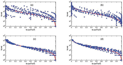Then, the scaled curve is drawn for each of the different soil and scaling methods. Figure 1 shows the water retention curve calculated with the lognormal equation (unscaled) and the scaled equation using the three methods: Kosugi and Hopmans (Tuli et al. 2001), the proposed method, and the optimization method. Figure 1(b) shows that the Kosugi and Hopmans (1998) method failed to scale the soil water retention curve properly. Table 2 shows a comparison of statistical parameters before and after scaling with the three different methods. The results of Table 2 show that the RMSE value before scaling was 0.293 and after scaling with Kosugi and Hopmans (1998), the RMSE value reached 0.225. The SE value obtained with this method is 23.2%. Although scaling using the Kosugi and Hopmans (1998) method has reduced the scattering of points around the reference curve, this reduction has not been noticeable. Because the Kosugi and Hopmans (1998) method leads to satisfactory results only for similar soils (with an almost equal value of σ; Sadeghi et al. 2016), the selection of these soils (with a coefficient of variation for σ of about 58%) combined with this method of scaling has not produced the desired results in this study.

Table 2. Statistical results of different methods used for scaling

Method	RMSE	SE(%)	R^2
Unscaled	0.293	-	0.67
Kosugi and Hopmans	0.225	23.2	0.75
Proposed	0.093	68.2	0.98
Optimized	0.083	70.4	0.97

Figure 1. Water retention curve calculated and scaled in different ways: (a) unscaled; (b) scaled using the Kosugi and Hopmans method; (c) scaled using the proposed method; (d) scaled using the optimum method.

: reference curve

In the proposed method, using Equation (9)(9) ${\alpha }_i={\left(\frac{\mathrm{l}\mathrm{n}\left(S_{e_i}\right)}{\mathrm{l}\mathrm{n}\left(S_{e_{ref}}\right)}\right)}_{hi}$(9) and effective saturation in the suction of 1000 cm for the reference soil and the desired soil, the scaling factor for different soils was obtained. After determining the scaling factor, the scaled water retention curve is drawn using Equation (10)(10) $S_{e_{ij}}^{\ast }=exp\left[\frac{\mathrm{l}\mathrm{n}\left(S_{e_{ij}}\right)}{{\alpha }_i}\right]$(10) . Figure 1(c) shows that the use of the proposed method has caused the data scattering to be reduced and brought it closer to the reference curve. Given the the fact that the scaling factor is based on the effective saturation of the 1000 cm suction ($S{e}_{1000}$), the values of the water retention curve for different textures pass through this point. The value of RMSE has reached 0.093 and the value of the coefficient of determination ($R^2$) has reached 0.98 (from 0.67 before scaling). The scaling efficiency in this method is 68.2%. The results show that the accuracy of the proposed method is higher than that of the Kosugi and Hopmans (1998) method.

At the same time, using the optimization method, the best factor for the proposed scaling method was obtained; the water retention curve scale for this method is shown in Fig. 1(d). With the optimization method, the RMSE value is 0.083 and the scale efficiency is 70.4%. The value of the coefficient of determination ($R^2$) of this method is equal to 0.97. Although the scale-up efficiency of the optimization method is higher than the scale-up efficiency of the proposed method (68%), this increase has not been noticeable. In general, it can be concluded that the proposed method scales the water retention curve with appropriate accuracy.

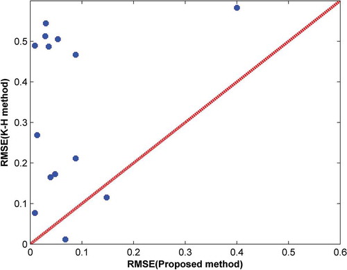
Figure 2 provides a visual comparison of the average error squares (RMSE) obtained by scaling the water retention curve for the proposed method and the Kosugi and Hopmans method relative to the 1:1 line in different soils. Figure 2 shows that in most soils the proposed method is much better than the Kosugi and Hopmans method of scaling for different soils. In soils 2491 and 4340, the RMSE obtained by the Kosugi and Hopmans method is less than that for the proposed method. The values of σ in soils 2491 and 4340 are 1.9 and 1.87, respectively, and are close to the value of σ in the reference curve (1.77), so the geometric similarity condition expressed by Das et al. (2005) is established in these soils. In general, this form shows the superiority of the proposed method over the Kosugi and Hopmans (1998) method in different soils.

Figure 2. RMSE values for the proposed method and the K-H method

3.2 The effect of selected moisture on the scaling factor

This section evaluates the effect of varying water contents in obtaining the scaling factor. Table 3 compares the scaling factor (${\alpha }_{ij}$) obtained with the proposed method based on the effective saturation $S{e}_{100},S{e}_{330},S{e}_{700},S{e}_{1000},S{e}_{5000},S{e}_{10000}$ compared with the optimization method (${\alpha }_{Opt}$). Using the proposed method, the lowest value of the scaling factor was 0.001 in soil 4611 at $S{e}_{100}$, and the highest value was 79.80 in soil 4443 at $S{e}_{1000}$. In the optimization method, the lowest scaling factor of 0.24 was found in soil 3395 and the highest scaling factor of 76.52 was obtained in soil 4443. In seven soils, the optimal scaling factor was less than 1, and in seven soils it was larger than 1; the pattern was almost the same for the proposed method. The value of the scaling factor obtained based on $S{e}_{5000}$ is closest to the scaling factor obtained based on the optimization method. The results show that the use of effective saturation data related to the middle water retention curve increases the accuracy of the proposed method. Kosugi and Hopmans (1998) and Tuli et al. (2001) used a moderate suction amount to scale the lognormal water retention curve. Khatri and Smith (2006) used the scaling factor to determine the equivalent infiltration parameters in furrow irrigation using scaling based on the progress distance to the middle of the furrow length. Chari et al. (2020) used the infiltrated amount of water after 240 min as a scaling factor.

Table 3. Scaling factor obtained in different suctions

Texture	100	330	700	1000	5000	10 000	${\alpha }_{opt}$
4443	60.45	-	-	-	-	-	76.52
3050	13.76	22.81	25.53	-	-	-	27.29
4445	6.58	18.54	23.57	25.29	-	-	29.23
3130	5.99	6.14	6.02	5.95	5.58	5.44	5.95
4611	0.001	0.02	0.11	0.23	0.55	0.77	0.72
3120	0.37	0.59	0.71	0.77	0.97	1.04	0.98
4512	0.67	0.84	0.92	0.95	1.07	1.10	1.06
4870	0.92	1.25	1.42	1.48	1.69	1.75	1.68
2491	1.07	1.00	0.97	0.95	0.93	0.92	0.93
1400	0.23	0.28	0.31	0.32	0.39	0.41	0.39
4340	1.61	1.41	1.31	1.28	1.17	1.14	1.18
4543	0.84	0.64	0.57	0.53	0.47	0.45	0.49
3380	1.09	0.79	0.69	0.64	0.54	0.51	0.57
3395	0.24	0.27	0.25	0.25	0.24	0.24	0.24

3.3 De-scaling

Figure 3 shows the amount of effective saturation calculated (real) and obtained using the de-scaling process (Equation (11)(11) $S_{e_{ji}}=exp\left[{\alpha }_{i}ln{\left(S_{e_r}\right)}_j\right]$(11) ) for the studied soils relative to the 1:1 line. 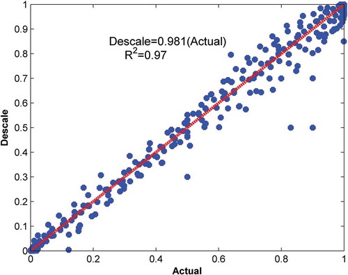In the de-scaling process, after calculating the scale factor (Equation (9)(9) ${\alpha }_i={\left(\frac{\mathrm{l}\mathrm{n}\left(S_{e_i}\right)}{\mathrm{l}\mathrm{n}\left(S_{e_{ref}}\right)}\right)}_{hi}$(9) ), using Equation (11)(11) $S_{e_{ji}}=exp\left[{\alpha }_{i}ln{\left(S_{e_r}\right)}_j\right]$(11) , the effective saturation curve is taken out of the scale mode and the effective saturation curve is plotted on its actual scale. Figure 3 shows that in most cases the points are close to the error one by one. The value of the coefficient of determining the amount of real effective saturation obtained using the scaling process is 0.98, which indicates the appropriate accuracy of the method proposed in this study. Figure 3 shows that the de-scaling method is more accurate at low moisture than at high moisture. Since the scale factor is selected based on the moisture in the 1000 cm suction, the water content obtained in the middle suction range and with low moisture is higher than with high moisture, due to the type of soil.

Figure 3. Calculated and obtained water contents using the de-scaling process for the studied soils

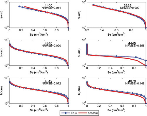
For a more comprehensive assessment of the method presented in this study, in Fig. 4, the relative saturation curves calculated using Equation (4)(4) $S_e=0.5erfc\frac{\mathrm{l}\mathrm{n}\left(h/h_{mi}\right)}{\sigma \sqrt{2}}$(4) and obtained using the de-scaling process (Equation (11)(11) $S_{e_{ji}}=exp\left[{\alpha }_{i}ln{\left(S_{e_r}\right)}_j\right]$(11) ) for soils with different and multiplied textures different similarities have been drawn. Figure 4 also shows the average value of the root of the error squares ($NRMSE=\frac{RMSE}{\bar{P}}$) for each of the figures. The highest accuracy is found in soil 3395 (with silt loam texture and σ = 3.01) with an NRMSE of 0.009. In this soil, the effective saturation value obtained using the de-scaling process is completely consistent with the actual data. The lowest accuracy was found in soil 4445 (with sand texture and σ = 0.34) with an NRMSE of 0.358. In this soil, because of its high moisture, the accuracy of the calculation method with the de-scaling process has been reduced. With the exception of soil 1400 (with clay texture and σ = 2.02), in other soils the effective saturation value obtained from the de-scaling process at high moisture is closer to the actual value. Given that Equation (11)(11) $S_{e_{ji}}=exp\left[{\alpha }_{i}ln{\left(S_{e_r}\right)}_j\right]$(11) uses 1000 cm suction to obtain the scale factor, the effective saturation value obtained in the middle suction ($S_e$ close to 1000 suction) is closest to the values obtained from Equation (4)(4) $S_e=0.5erfc\frac{\mathrm{l}\mathrm{n}\left(h/h_{mi}\right)}{\sigma \sqrt{2}}$(4) . In soils 4340 and 3395, the effective saturation value obtained from the de-scaling process is slightly higher than the actual value for values greater than $S{e}_{1000}$ and slightly lower than the actual value for values smaller than $S{e}_{1000}$. In other soils, Fig. 4 shows the opposite. This is because the scale of the proposed method (${\alpha }_{1000}$) in soils 4340 and 3395 is larger than the optimal scale factor (${\alpha }_{opt}$) (Table 3). In general, the results of Fig. 4 demonstrate the success of the proposed method for determining the water content in different soils.

Figure 4. Calculated and obtained effective saturation using Equation (11)(11) $S_{e_{ji}}=exp\left[{\alpha }_{i}ln{\left(S_{e_r}\right)}_j\right]$(11) for different soils

4 Conclusions

The application of physical scaling methods, such as those offered by Kosugi and Hopmans (1998), is limited to similar soil media. Also, most experimental methods (functional normalization) of non-comparable soil scaling based on minimizing the difference in squares (SSE) between the average water retention curve of soil water and water content data have been scaled. In the present research, a simple method for water retention curve scaling for different soils was presented. To obtain a water retention curve, a reference curve and the amount of moisture needed for a particular suction are required. The proposed method was evaluated for a wide range of soils. The results showed that if a relative saturation of $S{e}_{1000}$, $S{e}_{5000}$ and $S{e}_{10000}$ is used to obtain the scale factor, an answer close to the optimal scale factor is obtained. The results showed that the proposed method is more accurate than the Kosugi and Hopmans method (1998). Another application of the proposed method is to determine the water retention curve of soil water using the minimum field measurement (instead of measuring the water content at different suctions). The results showed that a water retention curve can be accurately predicted using a suction-water content measurement point and a reference curve. In general, it can be concluded that the proposed method accurately predicts the water retention curves of different soils.

Disclosure statement

No potential conflict of interest was reported by the authors.

Supplementary material

Supplemental data for this article can be accessed here.

Additional information

Funding

This work was supported by the University of Zabol [UOZ-GR-9618-122].

References

- Ahmadi, S.H., Sepaskhah, A.R., and Fooladmand, H.R., 2014. A simple approach to predicting unsaturated hydraulic conductivity based on empirically scaled microscopic characteristic length. Hydrological Sciences Journal, 60(2), 326–335. doi:10.1080/02626667.2014.959445
- Ahuja, L.R. and Williams, R.D., 1991. Scaling water characteristics and hydraulic conductivity based on Gregson-Hector-Mcgowab approach. Soil Science Society of America Journal, 55, 308–319. doi:10.2136/sssaj1991.03615995005500020002x
- Babaei, F., et al., 2018. Spatial analysis of infiltration in agricultural lands in arid areas of Iran. Catena, 170, 25–35. doi:10.1016/j.catena.2018.05.039
- Brooks, R.H. and Corey, A.T. 1964. Hydraulic properties of porous media. Hydrology Paper No. 3, Colorado State University, Fort Collins, 27p.
- Chari, M.M., et al., 2019. General equation for advance and recession of water in border irrigation. Irrigation and Drainage, 68 (3), 676–687. doi:10.1002/ird.2342
- Chari, M.M., Poozan, M.T., and Afrasiab, P., 2020. Modeling soil water infiltration variability using scaling. Biosystem Engineering, 196, 56–66. doi:10.1016/j.biosystemseng.2020.05.014
- Das, B.S., Haws, W.N., and Rao, P.S.C., 2005. Defining geometric similarity in soils. Vadose Zone Journal, 4, 264–270. doi:10.2136/vzj2004.0113
- Gregson, K., Hector, D.J., and McGowan, M., 1987. A one-parameter model for the soil water characteristic. Journal of Soil Sience, 38, 483–486. doi:10.1111/j.1365-2389.1987.tb02283.x
- Hendrayanto, K., Kosugi, K., and Mizuyama, T., 2000. Scaling hydraulic properties of forest soils. Hydrological Process, 14, 521–538. doi:10.1002/(SICI)1099-1085(20000228)14:3<521::AID-HYP952>3.0.CO;2-C
- Khatri, K.L. and Smith, R.J., 2006. Real-time prediction of soil infiltration characteristics for the management of furrow irrigation. Irrigation Science, 25 (1), 33–43. doi:10.1007/s00271-006-0032-1
- Kosugi, K. and Hopmans, J.W., 1998. Scaling water retention curves for soils with lognormal pore-size distribution. Soil Science Society of America Journal, 62, 1496–1504. doi:10.2136/sssaj1998.03615995006200060004x
- Kozak, J.A. and Ahuja, L.R., 2005. Scaling of infiltration and redistribution of water across soil textural classes. Soil Science Society of America Journal, 69 (3), 816‐827. doi:10.2136/sssaj2004.0085
- Meskini-Vishkaee, F., Mohammadi, M.H., and Vanclooster, M., 2014. Predicting the soil moisture retention curve, from soil particle size distribution and bulk density data using a packing density scaling factor. Hydrology and Earth System Sciences, 18, 4053–4063. doi:10.5194/hess-18-4053-2014
- Miller, E.E. and Miller, R.D., 1956. Physical theory for capillary flow phenomena. Journal of Applied Physics, 27 (4), 324–332. doi:10.1063/1.1722370
- Nasta, P., et al., 2009. Scaling soil water retention functions using particle-size distribution. Journal of Hydrology, 374, 223–234. doi:10.1016/j.jhydrol.2009.06.007
- Nasta, P., Romano, N., and Chirico, G.B., 2013. Functional evaluation of a simplified scaling method for assessing the spatial variability of soil hydraulic properties at the hillslope scale. Hydrological Sciences Journal, 58 (5), 1059–1071. doi:10.1080/02626667.2013.799772
- Nemes, A., et al., 2001. Description of the unsaturated soil hydraulic database UNSODA. Version 2.0, Journal of Hydrology, 251, 151–162. doi:10.1016/S0022-1694(01)00465-6
- Pollacco, J.A.P., et al., 2017. Saturated hydraulic conductivity model computed from bimodal water retention curves for a range of New Zealand soils, Hydrology and Earth System Sciences, 21, 2725–2737. doi:10.5194/hess-21-2725-2017
- Rieu, M. and Sposito, G., 1991. Fractal fragmentation, soil porosity and soil water properties: i. Theory. Soil Science Society of America Journal. Soil Science Society of America, 55, 231–1238.
- Sadeghi, M., et al., 2016. A critical evaluation of the Miller and Miller similar media theory for application to natural soils. Water Resources Research, 52 (4), 1–18. doi:10.1002/2015WR017929
- Sadeghi, M., et al., 2012. Additional scaled solutions to Richards’ equation for infiltration and drainage. Soil and Tillage Research, 119, 60–69. doi:10.1016/j.still.2011.12.004
- Sharma, M.L., Gander, G.A., and Hunt, C.G., 1980. Spatial variability of infiltration in a watershed. Jornal of Hydrology, 45, 122–101.
- Simmons, C.S., Nielsen, D.R., and Biggar, J.W., 1979. Scaling of field-measured soil-water properties. Hilgardia, 47, 77–173.
- Tillotson, P.M. and Nielsen, D.R., 1984. Scale factors in soil science. Soil Science Society of America Journal, 48(5), 953‐959. doi:10.2136/sssaj1984.03615995004800050001x
- Tuli, A., Kosugi, K., and Hopmans, J.W., 2001. Simultaneous scaling of soil water retention and unsaturated hydraulic conductivity functions assuming lognormal pore-size distribution. Advances in Water Resources 24, 677–688. doi:10.1016/S0309-1708(00)00070-1
- Tyler, S.W. and Wheatcraft, S.W., 1990. Fractal processes in soil water retention. Water Resources Research, 26 (5), 1047‐1054. doi:10.1029/WR026i005p01047
- Vogel, T., Cislerova, M., and Hopmans, J.W., 1991. Porous media with linearly hydraulic properties. Water Resources Research, 27 (10), 2735–2741. doi:10.1029/91WR01676
- Warrick, A.W., Mullen, G.J., and Nielsen, D.R., 1977. Scaling of field measured hydraulic properties using a similar media concept. Water Resources Research, 13 (2), 355–362. doi:10.1029/WR013i002p00355
- Warrick, A.W. and Nielsen, D.R., 1980. Spatial variability of soil physical properties in the field. In: D. Hillel, ed. Applications of soil physics. New York: Academic Press, 319–344.
- Williams, R.D. and Ahuja, L.R., 2003. Scaling and estimating the soil water characteristic using a one‐parameter model. In: Y. Pachepsky, D.E. Radcliffe, and H.M. Salim, eds. Scaling methods in soil physics. Boca Raton, FL: CRC Press, 35‐48.