Application of random forest and multi-linear regression methods in downscaling GRACE derived groundwater storage changes

ABSTRACT

The advent of Gravity Recovery and Climate Experiment (GRACE) has opened the doors for remote monitoring of gravitational changes and its derivatives across the globe, but received less attention due to poor spatial and temporal representation. Statistical models of varying complexity are commonly employed to downscale the GRACE datasets for use with local to regional applications. This study presents the application of two commonly employed machine learning models, multi-linear regression (MLR) and random forest (RF), in spatially downscaling (from 1° to 0.25°) the GRACE-derived terrestrial water storage anomalies (TWSA) by establishing a correlation with various land surface and hydroclimatic variables. The downscaled TWSA was further converted into groundwater storage anomalies. Applicability of the proposed methods was tested on four contrasting hydrogeological basins of India. For each basin, the significant predictor variables were considered to establish the relations. Seasonal groundwater levels observed in 236 wells during 2006–2015 were used for method validation and accuracy assessment. We observed a close match between GRACE-derived groundwater levels and the measurements for three of the four basins (r = 0.40–0.92, Root mean square error (RMSE) = 3.6–10.5 cm). Our results indicate that the predictor variables to downscale TWSA should be considered cautiously based on the hydrogeological, topographical, and meteorological characteristics of the basin.

KEYWORDS:

• GRACE
• statistical downscale
• multi-linear regression
• random forest
• groundwater storage
• India

Editor A. Fiori Associate editor S. Pingale

1 Introduction

Groundwater is the largest source of readily available freshwater in the world, accounting for about 30% (Gleik 1993). More than two billion people around the globe depend on the fresh aquifer reservoirs for their drinking needs, and about 43% of croplands are cultivated using groundwater (Siebert et al. 2010). Owing to its universal availability and low capital cost, groundwater is being extracted at a rate of about 1000 km³/year, far more rapidly than any other resource, thus resulting in a rapid depletion rate of about 350 km³/year (Aeschbach-Hertig and Gleeson 2012). India is the largest user of groundwater in the world, responsible for more than 25% of global groundwater abstraction (Chindarkar and Grafton 2019). Considering its ubiquitous nature and uninterrupted supply, groundwater has become the chief and most reliable source to supply the irrigation needs of the country. This is also evidenced by the 7-fold increase in net area irrigated by groundwater (from 5.98 Mha in 1951 to 42.44 Mha in 2013) against a mere 2-fold increase in net area irrigated by surface water during the same period (from 8.29 Mha to 16.28 Mha). More than 85% of India’s rural domestic water requirements, 50% of urban water requirements, and 50% of agricultural water requirements are met from groundwater reservoirs (Kulkarni et al. 2015).

Groundwater systems are highly dynamic to various external stresses including changes in climate, land use, withdrawals, and recharge mechanism (Meixner et al. 2016). The nature of stress and intensity experienced by an aquifer are dependent on geographical location, layer stratigraphy, meteorological conditions, demographics, and water demand for various uses. If the current rate of groundwater extraction continues, it may result in an unsustainable balance, leading to poverty and food insecurity in many parts of the country (Girotto et al. 2016, Zaveri et al. 2016). Periodic monitoring of groundwater levels through a network of observation wells is the principal source of information to predict the aquifer response to such hydrological stresses (Taylor and Alley 2001). Long-term, systematic monitoring of groundwater levels can help hydrogeologists, water managers, and modellers in the effective management of groundwater resources (Taylor and Alley 2001).

In India, the Central Ground Water Board (CGWB) is the apex body that monitors the groundwater levels, four times a year (in January, May, August, and November) using a network of about 15 500 observation wells (10 715 dug wells and 4938 piezometers). The distribution of observation wells throughout the country is highly non-uniform, ranging from a very low density in the northeast region to a very high density in the southern region. This spatial heterogeneity and the inadequacy of the monitoring well network limit its use in groundwater resource estimation and management; however, these limits can be overcome using remote sensing techniques and measurements (Rahaman et al. 2019).

The gravity recovery and climate experiment (GRACE) satellite mission was launched in 2002, with the goal of monitoring the Earth’s gravitational field at a spatial resolution of 400–40 000 km, a temporal resolution of 30 days, and a measurement accuracy of 1 μGal (Tapley et al. 2004). The GRACE mission consists of twin satellites separated by a distance of 220 km, moving in a near-circular, low-earth orbit (altitude: ~ 500 km), at an inclination of 89.5°. The inter-satellite distance and their relative positions are precisely measured using a radar telemeter operating in the K-band of the microwave region, and this information is converted into the gravitational acceleration anomalies. GRACE data is generally presented in the form of terrestrial water storage anomalies (TWSAs) for use with hydrological applications at regional to continental scales (Flury et al. 2008). The reported TWSA is composed of all possible contributing water masses (snow, biomass, canopy water, surface water, soil moisture, and groundwater) contained in the soil column of a given GRACE cell (Chen et al. 2014, Frappart and Ramillien 2018). GRACE is distinct from conventional land observation satellite systems, as (i) it uses two co-orbital satellites, and acquires data in the microwave band; (ii) it does not contain optical sensors to capture the reflected or emitted electromagnetic radiation from the land surface; and (iii) the data is not contaminated by the presence of clouds or atmospheric noise. Applications of GRACE range across a number of domains including geophysics, geodesy, hydrology, groundwater, and oceanography (Jiang et al. 2014, Shen et al. 2014, Nanteza et al. 2016, Ariege 2018). Despite its high measurement accuracy, GRACE’s applications are limited due to its poor spatial representation, thus requiring downscaling before it can be used with groundwater monitoring and management applications at local to regional scales (Chen et al. 2019).

Downscaling of GRACE-derived TWSA can happen at three levels: (i) spatial downscaling, wherein the coarse-resolution TWSA (~ 110 km) is disaggregated into finer resolution (hundreds of metres) for use with local to regional applications; (ii) temporal downscaling, wherein the monthly-averaged TWSA from GRACE is partitioned into diurnal variations; and (iii) vertical downscaling, where in the TWSA is disaggregated into the contributing fluxes (such as canopy water storage, soil moisture, surface water storage, and groundwater storage) for use in hydrological applications (Reager et al. 2015). Inspired by climate modelling studies, spatial downscaling of GRACE-derived TWSA data can be performed using dynamic or statistical techniques. Dynamic downscaling assimilates the low-resolution TWSA into a high-resolution, physically based land surface model (LSM) to derive the high-resolution data (Rahaman et al. 2019). The physical processes of the LSMs and the atmospheric forcing in conjunction with ensemble data assimilation systems are used to distribute GRACE data into finer scales (Miro and Famiglietti 2018).

A number of researchers have successfully downscaled GRACE data dynamically (Fersch et al. 2012), with the objective to (i) improve drought simulations within the Murray-Darling Basin in Australia (Schumacher et al. 2018); (ii) improve water storage and flux simulations in the Mississippi River Basin (Zaitchik et al. 2008); and (iii) develop drought indicators for the North American region (Houborg et al. 2010). In spite of their strong advantage of being physically consistent, dynamic downscaling techniques commonly suffer from the drawbacks of computational complexity, require extensive datasets from multiple sources, and demand a detailed gauge-wise monitoring network (Rahaman et al. 2019).

In contrast, statistical downscaling methods use local observations made over longer time periods to establish the empirical relationships between the coarse-scale input data (predictors) and the fine-scale target datasets (predictands) (Yin et al. 2018). These methods can capture the underlying physical dynamics of the system using data-driven non-parametric models or transfer functions (Sun et al. 2010). Statistical downscaling techniques are relatively flexible, simple to use, and computationally inexpensive, and hence outperform dynamical downscaling methods in terms of their applicability and parameter estimation (Liu et al. 2016). A number of statistical techniques, including classification-based methods, regression models, Markov chains, and conditional expectation models have been successfully applied to downscale GRACEderived TWSA data for groundwater applications (Ning et al. 2014, Gemitzi and Lakshmi 2018).

Advanced statistical models that create an ensemble of learning models from the vast datasets, commonly referred as machine learning (ML) algorithms, have gained popularity in recent years to downscale the GRACE data (Chen et al. 2019, Rahaman et al. 2019, Seyoum et al. 2019). Miro and Famiglietti (2018) applied artificial neural networks (ANN) to downscale GRACE products in California’s central valley to better understand the spatial groundwater levels. Yin et al. (2018) developed a multi-linear regression model between GRACE-derived GWSA and Moderate Resolution Imaging Spectroradiometer (MODIS)-derived evapotranspiration (ET) datasets, and were able to capture the sub-grid heterogeneity in groundwater storage changes (at 2 km resolution) for the North China Plain aquifer. However, their method can be extended to only those regions, that exhibit a good correlation between GWSA and ET at a coarse scale. Rahaman et al. (2019) applied a supervised ML algorithm, viz. a random forest (RF) approach, to develop fine-scale (0.25°) groundwater storage anomaly (GWSA) maps for the Northern High Plains aquifer in the USA. Their model successfully predicted the seasonal as well as long-term trends of GWSA at finer resolution. Seyoum et al. (2019) applied a two-stage boosted regression tree ML method to predict groundwater level anomalies (GWLAs) at 0.25° resolution for the Illinois watershed. Verma and Katpatal (2020) applied ANN to validate the sensitivity of GRACE data to groundwater storage variations by considering the heterogeneity in basin characteristics for the basaltic aquifer systems of India.

Despite the aforementioned studies, the dependence of various hydroclimatic forcing factors (such as precipitation, temperature, soil moisture, evapotranspiration, base flows) on the downscaling mechanism, in relation to the hydrogeological setting, remains unclear. Hence, the specific objectives of this study are to:

1. Spatially downscale the GRACE-derived TWSA data (from 1° to 0.25°) using two commonly employed ML techniques (multi-linear regression and random forest);

2. Test the applicability of the proposed algorithms on four contrasting hydrogeological basins of India using observed groundwater levels; and

3. Evaluate the role of various hydroclimatic forcing factors on the downscaling strategy for each basin and exploit the associated relation.

2 Methodology

2.1 Study area

Four principal aquifer systems of India, that differ in terms of geographical location, hydrogeology, groundwater withdrawals, and aquifer recharge mechanisms, were considered to test the robustness of the proposed algorithms in predicting the regional groundwater level as well as the storage changes (Fig. 1). These systems were:

1. Unconsolidated river alluvia (AL) of northern India,

2. Semi-consolidated sandstone sediments (ST) of northwestern India,

3. Deccan trap basaltic aquifers (BS) of western India, and

4. A consolidated granite–gneiss complex (GN) of eastern India.

Figure 1. Location map showing the hydrogeological formations used in this study. The 1° GRACE cells (red squares) and the observation wells used in the model validation (filled circles) are superimposed on the aquifer maps

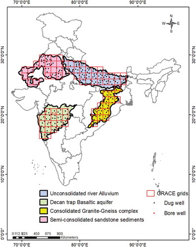
Hydrogeological and land-use characteristics of each basin are provided in Table 1. Unconsolidated river alluvium (AL) forms an integral part of the Ganga River basin, which experiences a subtropical humid climate with a mean annual rainfall range of 600–1400 mm (Misra 2013). This region is densely populated and cultivated due to the presence of fertile lands, favourable agro-climatic conditions, and perennial water systems. Depth to groundwater is predominantly shallow, with the aquifer directly recharged by the monsoonal rainfall and agricultural return flows (CGWB 2012). The semi-consolidated sandstone basin (ST) experiences an arid climate and receives a mean annual rainfall of 100–150 mm (Prajapat and Choudhary 2018). The aquifer thickness ranges from 40 to 80 m, with well yields ranging from 100 to 150 m³/h. Agriculture is confined to the eastern part of the region, due to the presence of thick alluvial sediments. Deccan trap basalts (BS) are characterized by multiple layers of solidified flood basalt resulting from volcanic eruptions. This region is characterized by a semi-arid climate with mean annual rainfall ranging from 600 mm in the rain shadow belt of the western Ghats to 2000 mm in the coastal region (Verma et al. 2020). The thickness of the aquifer ranges from 5 to 18 m, with dug well yields ranging from 0.2 to 30 m³/h. The consolidated granite–gneiss complex (GN) comprises crystalline formations of Precambrian age. The climate of the region is predominantly subtropical, with a mean annual rainfall of 1300 mm. Aquifers of this region are weathered to fractured with a thickness range of 10–60 m, and a discharge range of 10–30 m³/h (CGWB 2012).

Table 1. Geographical, hydrogeological, and land-use characteristics of the basins considered in this study

Basin	River alluvium	Sedimentary sandstone	Deccan trap basaltic	Crystalline formation with granite-gneiss
Abbreviation	AL	ST	BS	GN
Area (km^2)	288 660	241 044	253 738	169 023
Latitude range	26°30'30” –29°44'56”N	24°43ʹ24”–30°8ʹ2”N	16°7ʹ50”–21°4ʹ29”N	17°59ʹ4”–24°12ʹ29”N
Longitude range	77°9'38” –88°11'11”E	69°27ʹ29”–78°13ʹ7”E	73°29ʹ1”–77°56ʹ29”E	81°12ʹ2”–87°0ʹ4”E
Geological age	Quaternary (young to old alluvium)	Upper Paleozoic to Cenzoic	Mesozoic to Cenzoic	Azoic to Proterozoic
Land uses	Agriculture (38.5%), forest (13.6%), urban (6.8%), water (17.9%), misc. (23.2%)	Agriculture (21%), forest (10.3%), urban (2.6%), water (3.3%), misc. (62.9%)	Agriculture (22.9%), forest (37.9%), urban (3.2%), water (6.6%), misc. (29.3%)	Agriculture (39.1%), forest (25.2%), urban (7.3%), water (19.3%), misc. (8.9%)
Administrative states	Uttar Pradesh, Bihar	Rajasthan, Punjab	Maharashtra	Odisha, Jharkhand
No. of GRACE cells	27	20	19	15

2.2 Data acquisition and processing

The release-06 (v. 3), level-3, GRACE-derived equivalent water thickness values representing TWSA for the Indian subcontinent were obtained in netCDF format for the period 2006–2015 and clipped to the study region. The data is presented in a grid format at 1° (~ 110 km) spatial and monthly temporal resolutions. A total of 120 time-series images (107 downloaded and 13 linearly interpolated), each containing 27, 20, 19, and 15 one-degree spatial GRACE cells, respectively, for the AL, ST, BS, and GN basins were used in the analysis (Fig. 1). The released version incorporates glacial isostatic adjustment (GIA) and standard corrections for geocentre (degree-1), C20 (degree-2), and C30 (degree-3), and applies post-processing filters to reduce the correlated errors. Data from all three official processing centres, namely CSR (Center for Space Research, Austin, United States), GFZ (GeoForschungsZentrum, Potsdam, Germany), and JPL (Jet Propulsion Laboratory, California, United States) were used in this study. Since the variability in the gravity fields obtained from the three sources (CSR, GFZ, JPL) is low (< 1.8 ± 0.8 mm), the ensemble mean was used in downscaling to reduce the noise in the gravity field solutions (Sakumura et al. 2014).

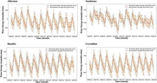
Figure 2 describes the monthly variations in TWSA for all the basins as observed by GRACE. The temporal patterns in TWSA are similar between years but differ in amplitude across the basins. The highest TWSA variation was observed for the GN basin (24.9 ± 2.1 cm), followed by AL (23.1 ± 1.8 cm), BS (15.9 ± 1.4 cm), and ST (12.9 ± 1.1 cm). The high variations for the GN basin could be due to its high dependency on surface water resources. The observed GWSA anomalies in TWSA as obtained from GRACE include vertically integrated measures of water storage changes in surface water, groundwater, soil moisture, snow water equivalent, and canopy water storage (Yin et al. 2018). GWSA followed a similar trend, with a phase difference of about 6 months. Overall, both TWSA and GWSA show a consistent decreasing trend with time.

Figure 2. Seasonal changes in terrestrial water storage anomalies (TSWAs) and groundwater storage anomalies (GWSAs) derived from GRACE (at 1° resolution) for different hydrogeological basins. Vertical bars represent the standard deviation around the mean

The Global Land Data Assimilation System (GLDAS) integrates satellite and ground-based observational data products using advanced land surface modelling and data assimilation techniques and generate optimal fields of land surface states and fluxes (Rodell et al. 2004). GLDAS provides high-quality land-surface fields using four LSMs, namely VIC (Variable Infiltration Capacity), NOAH, Mosaic, and CLM (Community Land Model). GLDAS-1 provides hydrological and meteorological datasets at 1° spatial resolution from all the LSMs, whereas GLDAS-2 provides data from the NOAH model alone at 0.25° resolution (Yin et al. 2018). The 3-h GLDAS data products are temporally aggregated to monthly interval to match with the GRACE products (Wang et al. 2016). Considering its ability to represent the land surface fields both at coarse (1° × 1°) and fine (0.25° × 0.25°) resolutions, and its effectiveness to represent the India Meteorological Department (IMD) observed precipitation datasets (Pai et al. 2014) for the four basins ($R_{AL}^2=0.92,R_{ST}^2=0.61,R_{BS}^2=0.85,R_{GN}^2=0.77)$, we used NOAH 2.1 model outputs in this study.

The predictor variables considered for each basin include precipitation (P), evapotranspiration (ET), bare soil evaporation (BE), soil moisture (SM), surface runoff (SR), subsurface runoff (SSR), canopy water storage (CWS) and canopy water evaporation (CWE). The variables considered in this study are mainly the hydrometeorological variables obtained from LSMs, as the extraction of variables from a single source will ensure less uncertainty and spatial mismatch. Additionally, MODIS imagery (MOD11B, L3, V6) was used to extract the monthly land surface temperature (LST) at both 0.25° and 1° spatial resolutions. The model predictors are converted into their respective anomalies by deducting the long-term mean of each parameter from the individual value. For example, the soil moisture anomaly for a given month “t” (∆SM_t) is given by:

(1) $\mathrm{\Delta }\mathrm{S}\mathrm{M}\mathrm{t}=\mathrm{S}\mathrm{M}\mathrm{t}-\overline{S{M}_{2006-15}}$(1)

where, SM_t is the soil moisture for the month t, and $\overline{S{M}_{2006-15}}$ is the mean value of soil moisture during the observation period (2006–2015).

2.3 Spatial downscaling of TWSA

2.3.1 Random forest (RF) algorithm

RF is a supervised, data-driven, machine-learning algorithm developed for classification and regression-based problems (Svetnik et al. 2003). The method allows non-linear interactions that can be learned from the data without explicitly modeling them (Grömping 2009). RF combines multiple decision trees, with each tree developed using randomly selected subsets of training samples and variables through replacement, hence yielding better results (Breiman 2001, Belgiu and Drăgu 2016). The individual trees are trained with two-thirds of the data, and the remaining one-third of the data, known as out of bag (OOB), is used for model validation. The parameters to be optimized during model development include: (i) the number of regression trees grown, based on the bootstrap sampling (ntree); (ii) the number of predictors tested at each node (mtry); and (iii) the minimum size of the terminal nodes of the trees (Mutanga et al. 2012). To improve the model performance, hyper parameters (such as the maximum depth of the trees to grow, and the minimum leaf samples) are selected using a 5-fold cross-validation technique. The variable importance calculated based on the variance is an important feature in RF that will make a significant contribution to the prediction. The variables that have low predictive power are neglected to improve the performance and ease the simulations. The ensemble mean of all trees as generated by RF is considered the model prediction and is run at finer resolution using the predictor variables, to generate high-resolution TSWA maps. RF was found to achieve good predictive performance with low overfitting and easy interpretability (Qi 2012).

2.3.2 Multi-Linear Regression (MLR) algorithm

MLR fits a regression line between the predictand (TWSA) and the predictors through a multidimensional space of data points. This method considers little or no multi-collinearity, and assume the regression residuals to be normally distributed. The dataset is divided into training and testing samples in a 70:30 ratio. Care was taken to maintain the same statistical parameters (mean and deviation) between the two samples. Considering the most significant predictors, MLR models were developed for each basin using the training set and evaluated using the testing set. The associated relation was further applied at fine (0.25° spatial) resolution to capture the sub-grid heterogeneity in TWSA.

2.4 Groundwater storage estimation and monitoring

ML algorithms predict TWSA at 0.25° resolution, using linear and/or non-linear relations, by considering the most important predictor variables. The sample space of variables under consideration include P, ET, BE, SM, SR, SSR, CSW, CWE and LST. GWSA at 0.25° resolution is then obtained by performing vertical water balance for each sub-grid cell, as below:

(2) $GWSA=TWSA-\left(\mathrm{\Delta }SM+\mathrm{\Delta }CSW+\mathrm{\Delta }SW+\mathrm{\Delta }SNW\right)$(2)

where $GWSA$ is the groundwater storage anomaly;$SA$ is the GRACE-downscaled terrestrial water storage anomaly; $\mathrm{\Delta }SM$, $\mathrm{\Delta }CSW$, and $\mathrm{\Delta }SNW$ are, respectively, soil moisture anomaly, canopy surface water anomaly, and snow water anomaly derived from the NOAH 2.1 model; and $\mathrm{\Delta }SW$ is the surface water anomaly obtained by aggregating the reservoir storage data available at the India Water Resources Information System (WRIS) website (http://indiawris.gov.in/wris/#/Reservoirs). Even though soil moisture (SM) was found to contribute significantly to TWSA in semi-arid environments, we relied on land surface model outputs for SM due to the absence of a dense monitoring network.

In situ groundwater levels at the 236 CGWB observation wells during the study period form the monitoring network for evaluating the proposed methods (source: https://indiawris.gov.in/wris/#/groundWater). Since CGWB monitors groundwater levels 4 times a year (January, May, August, and November), each gauge station has 40 time-varying observations during the study period. Spatio-temporal consistency in the data was ensured while selecting the monitoring stations. Data from multiple wells contained by each sub-grid cell (at 0.25° resolution) were averaged for use with comparison. The number of monitoring wells used in validation for the AL, ST, BS, and GN basins was, respectively, 88, 54, 49, and 45. The water table elevation (ground surface elevation minus observed water level) at each monitoring well was used to represent the water column height, and then converted into groundwater level anomalies (GWLA) by removing the long-term mean as follows:

(3) $GWL{A}_t=GW{L}_t-\overline{GW{L}_{2006-15}}$(3)

where $GWL{A}_t$ is the groundwater column height anomaly for the month t, $\overline{GW{L}_{2006-15}}$ is the groundwater column height observed for the month t, and $GWL{A}_t$ is the mean groundwater column height at the well location for the period 2006–2015. GWLA_t were converted into GWSA_t by multiplying by the specific yield (Sy) of the basin.

2.5 Performance evaluation

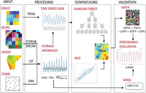
The best-performing ML algorithm was further considered to predict local-scale GWSA at 0.25° spatial resolution. Temporal patterns of GRACE-downscaled GWSA for each sub-grid cell were compared with well observations, and the deviations (or residuals) were analysed using statistical indicators. These included: (a) the correlation coefficient (r): a measure of interdependence of the two datasets, which ranges from −1 (perfect negative relation) to 0 (no relation) to +1 (perfect positive relation); (b) the root mean square error (RMSE): a measure of the standard deviation of the residuals from the best fit line; and (c) the Nash-Sutcliffe efficiency coefficient (NSE): a measure of the predictive power of the proposed model, which ranges from −∞ (poor prediction) to 0 (predicting the data mean) to +1 (perfect prediction). Specific yield (Sy) is a spatially heterogeneous parameter; hence, considering a unique value for the entire basin as suggested by CGWB can often mislead the results. The model sensitivity to Sy was analysed for each basin, and the optimal values for each sub-grid that result in a close match with observed water levels were reported. The input data requirement and anomaly estimation, along with the workflow of downscaling methodologies with their performance evaluation, are outlined in Fig. 3.

Figure 3. Workflow of the processes used in this study, showing the input data sources, anomaly estimation, downscaling algorithms, and performance evaluation using statistical indicators

3 Results and discussion

3.1 Selection of skilful predictors

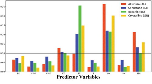
We considered nine hydrometeorological variables to investigate their role in downscaling the TWSA for each basin. These were: bare soil evaporation (BE), canopy water storage (CWS), canopy water evaporation (CWE), evapotranspiration (ET), precipitation (P), land surface temperature (LST), soil moisture (SM), surface runoff (SR), and sub-surface runoff (SSR). A total of 9720 temporal grid cells (with 3240 from AL, 2400 from ST, 2280 from BS, and 1800 from GN) were split sampled between training and testing datasets in a 70:30 ratio. Training data was used to establish the linear and non-linear relations (between TWSA and the predictors) at coarse resolution, while testing data was used to evaluate the developed relation. The importance of each variable is ascertained by estimating the decrease in the prediction accuracy in the absence of that variable. Figure 4 shows the normalized variable importance of the predictors (VIMP) in downscaling TWSA. It can be observed that the predictive power of each variable deviates slightly between the basins. A threshold VIMP of 0.10 was used to discard the variables having low predictive power. Of the nine variables under consideration, only four (ET, LST, SM, and SSR), with different strengths, were observed to be significant in downscaling the TWSA for all the basins. The cumulative contribution of all variables that were not included in the downscaling methodology for the AL, ST, BS, and GN basins is, respectively, 0.3, 0.34, 0.22, and 0.29. As the relations are developed by considering the temporal signatures of TWSA, we have ignored the effect of static variables such as digital elevation model (DEM) and slope from our analysis. Due to intense agriculture practices and aquifer–stream cross-flows, ET, SM, and SSR strongly influence TWSA for the AL basin. For the ST and BS basins, ET, SM, LST, and SSR are found to correlate highly with TWSA. Similarly, for the GN basin, TWSA shows a strong dependency on SM, LST, and SSR.

Figure 4. Histogram showing the normalized variable important measures of the predictors (VIMPs) for all basins. A threshold VIMP of 0.1 was used to discard the low-impact variables while downscaling the GRACE data to higher resolution

3.2 Inter-model comparison of downscaling relations

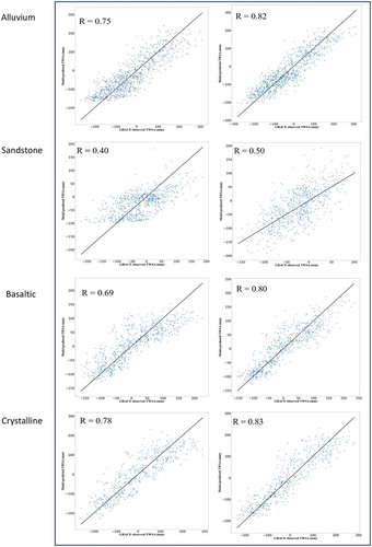
Considering the variables with high predictive power, both linear (MLR) and non-linear (RF) relations were established using the training datasets for each basin. The accuracy of each method was assessed by comparing model-derived TWSA estimates with GRACE measurements for the testing datasets (Fig. 5). The best-fit regression lines were forced to pass through the origin with a unit slope, for ease of comparison. Table 2 provides the distribution of TWSA data as well as the residual statistics in downscaling the TWSA for each basin. Both the highest positive (268 ± 0.78 mm) and the highest negative (−205 ± 0.45 mm) amplitudes in TWSA were observed for the AL basin. Irrespective of the basin characteristics, RF consistently outperformed MLR in estimating the TWSA at coarse (1° spatial) resolution. However, both RF and MLR have poorly represented the TWSA for the ST basin. Both models are overpredicting at low TWSA (−200 to −100 mm) and underpredicting at high TWSA (>200 mm). This could be due to ignorance of few basin-relevant predictor variables such as BE and P. Considering its ability to effectively predict TWSA changes at high resolution, only the RF method was considered further in downscaling and analysing the temporal trends in GWSA.

Table 2. Model performance of MLR and RF algorithms in downscaling TWSA for each basin

Basin	Multi-linear regression model			Random forest algorithm
	R (−)	RMSE (mm)	NSE	R (−)	RMSE (mm)	NSE
AL	0.75	56	0.67	0.82	48	0.77
ST	0.40	52	−0.43	0.50	47	0.50
BS	0.69	43	0.56	0.80	36	0.75
GN	0.78	58	0.70	0.83	48	0.81

Figure 5. Scatter plots showing the performance of linear (MLR) and non-linear (RF) techniques in estimating TWSA from the most important predictor variables

3.3 Seasonal and annual patterns in GWSA

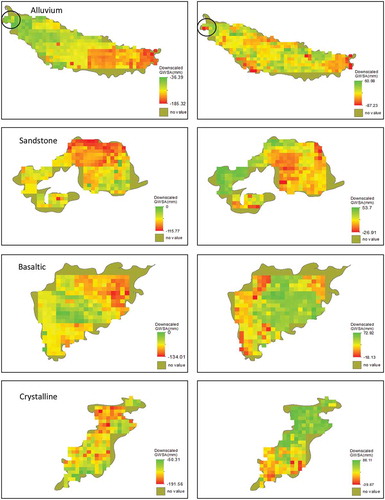
The study period (2006–2015) was further classified into dry (<25%), normal (25 to 75%), and wet (>75%) years based on the amount of precipitation received relative to the long-term mean. A total of 2 dry years (2010, 2013), 6 normal years (2006, 2007, 2009, 2011, 2012, 2015), and 2 wet years (2008, 2014) were observed. Basin-wise spatial trends in GWSA during pre- and post-monsoon seasons for a typical normal year (2011) are shown in Fig. 6. During this year, the cumulative precipitation received by AL, ST, BS, and GN basins was, respectively, 1066, 619, 1489, and 1349 mm (Pai et al. 2014). At the basin scale, GWSA for the AL basin consistently increased, from −185 ± 3.3 mm to 53 ± 2.1 mm. However, the southwest region experienced a decline in GWSA, by −7 ± 1.8 mm (circled in Fig. 6). This could be due to agricultural withdrawals in excess of recharge resulting from an extended crop period. In spite of scanty rainfall, the ST basin has experienced an increase in GWSA, with a mean value of 98 ± 2 mm. In contrast, the northern region situated in Punjab and Haryana experienced adrastic decline in GWSA, by −86 ± 1.7 mm. This is in accordance with the published literature (Rodell et al. 2009). For the BS basin, GWSA consistently increased, from −134 ± 2.68 mm to 72 ± 2.2 mm, due to monsoonal replenishment. The crystalline aquifer experienced a GWSA variation of −191 to −50 mm during pre-monsoon and −39 to +56 mm during post-monsoon, resulting in an overall increase in storage. We observed a close match between the regions of decreased GWSA (circled in Fig. 6) and the overexploited assessment units recommended by CGWB. The decline in GWSA is concentrated to the regions that depend exclusively on groundwater for their domestic and agricultural needs. We observed a basin-wide slight increase in GWSA from pre- to post-monsoon seasons during dry years, in spite of scanty rainfall and low monsoonal recharges.

Figure 6. Spatial distribution of downscaled groundwater storage anomalies (GWSAs) at the four hydrogeological basins during pre (left) and post (right) monsoon for a typical normal year (2011)

Temporal patterns in model-derived and observed GW levels for selective CGWB monitoring wells are shown in Fig. 7. A distribution free, non-parametric test was applied to estimate the trend in the dataset. To minimize the error in observations resulting from the uncertainty in specific yield estimates, we used groundwater levels for comparison instead of the commonly used GWSA (Rodell et al. 2009, Panda and Wahr 2016). For each basin, two representative wells, one with a flat and another with a steep water table gradient, were considered to see whether RF can predict both extremities in the anomalies. The RF method was able to replicate the groundwater level trends and seasonal variability but failed to simulate the peaks. The error in simulating GWLA peaks is significantly high (37%) for the ST basin.

Figure 7. Comparison of seasonal variations in downscaled (blue line) and observed (red line) groundwater level anomalies (GWLAs) for selective gauge stations across four basins of the study area

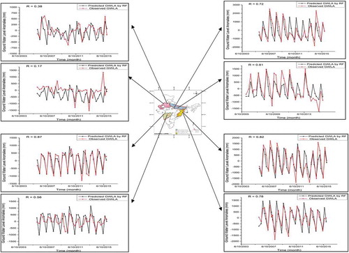
The predicted and observed GWLA cycles have the same alignment for all time periods except in the ST basin, for which the two cycles are slightly out of phase (r = 0.38). A sharp decline in GWSA, at a rate of −11.2 mm year⁻¹ during 2007–2010, was observed for the ST basin. Temporal patterns in GWSA revealed a clear seasonal variability, with the maximum occurring during August–September (post-monsoon) and the minimum occurring during May–June (pre-monsoon) for all basins. The mean peak-to-peak amplitude is highest for the AL basin (2233 mm), and lowest for the ST basin (422 mm). The observed (and RF-predicted, in parentheses) groundwater level depletion rates for the selected monitoring wells (Fig. 7) located in the AL basin were −5.09 cm year⁻¹ (−4.1 cm year⁻¹) and −7.2 cm year⁻¹ (−4.32 cm year⁻¹), in the ST basin were −1.4 cm year⁻¹ (−0.68 cm year⁻¹) and −5.6 cm year⁻¹ (−5.1 cm year⁻¹), in the BS basin were 3.2 cm year⁻¹ (2.1 cm year⁻¹) and −3.7 cm year⁻¹ (−2.95 cm year⁻¹), and in the GN basin were −2.2 cm year⁻¹ (−1.3 cm year⁻¹) and −3.9 cm year⁻¹ (−3.2 cm year⁻¹). Our results show that the proposed method can effectively capture both seasonal and annual trends in GWSA for the AL, BS, and GN basins.

3.4 Spatial distribution of GWSA

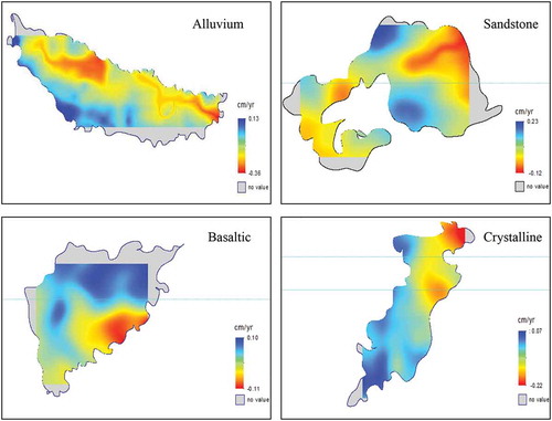
The spatial distribution of annual changes in GWSA averaged for the study period, using the best-performing RF model, are presented in Fig. 8. The average annual change (negative for decrease in storage and positive for increase in storage) in GWSA for the AL, ST, BS, and GN basins is, respectively, −1.7, 0.19, 0.15, and −0.34 mm year⁻¹. When converted to GWLA, these changes are, respectively, −14.7, 1.6, 1.2, and −2.8 mm year⁻¹. Our findings for the ST and BS basins are in agreement with the literature (Rodell et al. 2009, Verma and Katpatal 2020). The gains in storage volume by the ST and BS basins are, respectively, 0.4 and 0.38 km³, while the AL basin lost 4.9 km³ of storage volume during the study period, which is in agreement with other findings (Bhanja et al. 2020). In spite of an overall replenishment, the state of Uttar Pradesh in the AL basin has experienced a shortfall in GWSA (from −21 mm in 2006 to −42 mm in 2015) due to intense agriculture assisted with scanty rainfall. The northeastern and western part of the ST basin have seen a steady decline in groundwater levels due to intense agriculture and scanty rainfall. The southern part of the BS basin around Latur district has witnessed a sharp decline in groundwater levels due to acute drought conditions. The GWSA for the GN basin gradually increases from −0.22 cm year⁻¹ in the northern part to 0.38 cm year⁻¹ in the southern part. The calibrated Sy ranges for the AL, ST, BS, and GN basins are, respectively, 0.1–0.15, 0.1–0.15, 0.03–0.08, and 0.04–0.09. These values are within the specified ranges for the respective basins (Bhanja et al. 2016).

Figure 8. Mean annual changes in GRACE-derived GWLAs across all basins of the study area during 2006–2015. A positive value indicates a rise in the groundwater level, while a negative value indicates a fall in the groundwater level

3.5 Model validation and accuracy assessment

The performance of the RF method to simulate GWSA at sub-grid cell (0.25° spatial) resolution was evaluated using residual statistical parameters. The deviation in model-derived GWSA from the observations was analysed for each cell, and the associated correlation is presented in Fig. 9. Model cells that do not contain observation wells are excluded from the analysis (grey shaded). Similarly, data from multiple wells contained by a single cell were averaged for comparison. In general, the downscaled GWSA showed a good agreement with the observations. Out of 602 cells, 249 show a strong correlation (r > 0.6), 179 show a good correlation (0.4 < r < 0.6), and 174 show a poor correlation (r < 0.4). The RMSE values associated with predicting the GWSA for the AL, ST, BS, and GN basins are, respectively, 105, 43, 36, and 60 mm.

Figure 9. Choropleth map showing the spatial distribution of correlation coefficients between downscaled and observed GWSAs for each basin. Cells that do not contain observation wells are shaded in grey, and excluded from the analysis

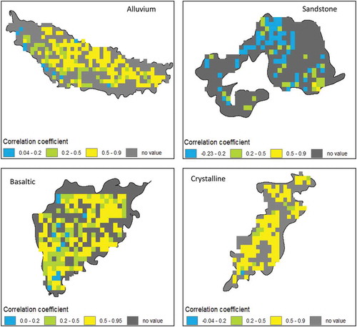
The percentage bias (PBIAS) estimates indicate that the model simulations are overpredicting by 4.7%, and 2.1% for the BS and GN basins, while underpredicting by 4.4% and 7.9% for the AL and ST basins. The NSE coefficients for predicting the GWSA for the AL, ST, BS and GN basins are, respectively, 0.51, 0.21, 0.76, and 0.63, which confirms that except for the ST basin, the magnitude of the residual variance is in agreement with the variance of the observations.

4 Conclusions

An accurate representation of groundwater trends and anomalies is a prerequisite to analyse the aquifer response subjected to various natural and anthropogenic stresses. The GRACE mission can help to improve the well monitoring network by estimating the groundwater changes from space. This study evaluates the performance of two ML algorithms, namely MLR and RF, in downscaling GRACE-derived TWSA (from 1° to 0.25°) and predicting GWSA at high (0.25°) spatial resolution.

The applicability of the proposed algorithm was tested using a 10-year (2006–2015) dataset from four contrasting hydrogeological basins of India. These were (i) river alluvia of northern India (AL), (ii) sandstone sediments of northwestern India (ST), (iii) basaltic aquifers of western India (BS), and (iv) crystalline formations of eastern India (GN). Except for the ST basin, RF consistently performed well in downscaling the TWSA data. The single exception may be due to our ignorance of anthropogenic fluxes (such as groundwater pumping, which is significant in the ST basin).

Only four predictor variables (ET, LST, SM, and SSR) were found to influence the downscaling relations for all of the basins. GRACE-derived groundwater levels agreed with the observations for 3 out of 4 basins, with acceptable errors (r = 0.40–0.92, RMSE = 3.6–10.5 cm, NSE = 0.21–0.76). GWSA was observed to be consistently decreasing for all the basins, at a rate ranging from −0.17 ± 0.01 cm year⁻¹ (AL) to 0.015 ± 0.01 cm year⁻¹ (BS). Cumulative annual depletions of groundwater from all of the basins amounts to 0.49 km³ year⁻¹ of water. The prediction accuracy is excellent except for the ST basin, as the observations for this basin do not represent the deep aquifer levels, from which groundwater is extracted. Our results indicate that RF, with basin-specific important predictors, can effectively capture the sub-grid heterogeneities and seasonal variations in GWSA derived from GRACE data.

Data availability

GRACE data is available at https://grace.jpl.nasa.gov/data/get-data/ and GLDAS data is available at https://disc.gsfc.nasa.gov/datasets?keywords=GLDAS. Other datasets that support this research work are available at the following link: https://jyolsnapj.github.io/GRACE/. If this link is inactive, the corresponding author can be contacted for the data files.

Disclosure statement

On behalf all authors, the corresponding author states that there is no conflict of interest.

References

- Aeschbach-Hertig, W. and Gleeson, T., 2012. Regional strategies for the accelerating global problem of groundwater depletion. Nature Geoscience, 5 (12), 853–861. doi:https://doi.org/10.1038/ngeo1617
- Ariege, 2018 May 2nd. Weighing earth, tracking water: hydrological applications of data from GRACE satellites. Available from: https://earth.yale.edu/sites/default/files/files/Ariege_Besson_Senior_Essay_2018.pdf.
- Belgiu, M. and Drăgu, L., 2016. Random forest in remote sensing: a review of applications and future directions. ISPRS Journal of Photogrammetry and Remote Sensing, 114, 24–31. doi:https://doi.org/10.1016/j.isprsjprs.2016.01.011
- Bhanja, S.N., et al., 2016. Validation of GRACE based groundwater storage anomaly using in-situ groundwater level measurements in India. Journal of Hydrology, 543, 729–738. doi:https://doi.org/10.1016/j.jhydrol.2016.10.042
- Bhanja, S.N., Mukherjee, A., and Rodell, M., 2020. Groundwater storage change detection from in situ and GRACE-based estimates in major river basins across India. Hydrological Sciences Journal, 65 (4), 650–659. doi:https://doi.org/10.1080/02626667.2020.1716238
- Breiman, L., 2001. Random forests. Machine Learning, 45 (1), 5–32. doi:https://doi.org/10.1023/A:1010933404324
- Chen, J., et al., 2014. Long-term groundwater variations in Northwest India from satellite gravity measurements. Global and Planetary Change, 116, 130–138. doi:https://doi.org/10.1016/j.gloplacha.2014.02.007
- Chen, L., et al., 2019. Downscaling of GRACE-derived groundwater storage based on the random forest model. Remote Sensing, 11 (24), 2979. doi:https://doi.org/10.3390/rs11242979
- Chindarkar, N. and Grafton, R.Q., 2019. India’s depleting groundwater: when science meets policy. Asia and the Pacific Policy Studies, 6 (1), 108–124. doi:https://doi.org/10.1002/app5.269
- Fersch, B., et al., 2012. Continental-scale basin water storage variation from global and dynamically downscaled atmospheric water budgets in comparison with GRACE-derived observations. Journal of Hydrometeorology, 13 (5), 1589–1603. doi:https://doi.org/10.1175/JHM-D-11-0143.1
- Flury, J., Bettadpur, S., and Tapley, B.D., 2008. Precise accelerometry onboard the GRACE gravity field satellite mission. Advances in Space Research, 42 (8), 1414–1423. doi:https://doi.org/10.1016/j.asr.2008.05.004
- Frappart, F. and Ramillien, G., 2018. Monitoring groundwater storage changes using the gravity recovery and climate experiment (GRACE) satellite mission: a review. Remote Sensing, 10 (6), 829. doi:https://doi.org/10.3390/rs10060829
- Gemitzi, A. and Lakshmi, V., 2018. Estimating groundwater abstractions at the aquifer scale using GRACE observations. Geosciences (Switzerland), 8 (11), 1–14. doi:https://doi.org/10.3390/geosciences8110419
- Girotto, M., et al., 2016. Assimilation of gridded terrestrial water storage observations from GRACE into a land surface model. Water Resources Research, 52 (5), 4164–4183. doi:https://doi.org/10.1002/2015WR018417
- Gleik, 1993. pdf. (n.d.).
- Grömping, U., 2009. Variable importance assessment in regression: linear regression versus random forest. American Statistician, 63 (4), 308–319. doi:https://doi.org/10.1198/tast.2009.08199
- Houborg, R., et al., 2010. Using enhanced GRACE water storage data to improve drought detection by the U.S. and North American drought monitors. International Geoscience and Remote Sensing Symposium (IGARSS), Honolulu, Hawaii, USA, 710–713. doi:https://doi.org/10.1109/IGARSS.2010.5654237
- Jiang, D., et al., 2014. The review of GRACE data applications in terrestrial hydrology monitoring. Advances in Meteorology, 2014, 1–9. doi:https://doi.org/10.1155/2014/725131
- Kulkarni, H., Shah, M., and Vijay Shankar, P.S., 2015. Shaping the contours of groundwater governance in India. Journal of Hydrology: Regional Studies, 4, 172–192. doi:https://doi.org/10.1016/j.ejrh.2014.11.004
- Liu, J., et al., 2016. Comparison of three statistical downscaling methods and ensemble downscaling method based on Bayesian model averaging in upper Hanjiang River Basin, China. Advances in Meteorology, 2016, 1–12. doi:https://doi.org/10.1155/2016/7463963
- Meixner, T., et al., 2016. Implications of projected climate change for groundwater recharge in the western United States. Journal of Hydrology, 534, 124–138. doi:https://doi.org/10.1016/j.jhydrol.2015.12.027
- Miro, M.E. and Famiglietti, J.S., 2018. Downscaling GRACE remote sensing datasets to high-resolution groundwater storage change maps of California’s central valley. Remote Sensing, 10 (1), 143. doi:https://doi.org/10.3390/rs10010143
- Misra, A.K., 2013. Climate change impact, mitigation and adaptation strategies for agricultural and water resources, in Ganga Plain (India). Mitigation and Adaptation Strategies for Global Change, 18 (5), 673–689. doi:https://doi.org/10.1007/s11027-012-9381-7
- Mutanga, O., Adam, E., and Cho, M.A., 2012. High density biomass estimation for wetland vegetation using worldview-2 imagery and random forest regression algorithm. International Journal of Applied Earth Observation and Geoinformation, 18 (1), 399–406. doi:https://doi.org/10.1016/j.jag.2012.03.012
- Nanteza, J., et al., 2016. Monitoring groundwater storage changes in complex basement aquifers: an evaluation of the GRACE satellites over East Africa. Water Resources Research, 52 (12), 9542–9564. doi:https://doi.org/10.1002/2016WR018846
- Ning, S., Ishidaira, H., and Wang, J., 2014. Statistical downscaling of Grace-derived terrestrial water storage using satellite and GLDAS products. Journal of Japan Society of Civil Engineers, Ser. B1 (Hydraulic Engineering), 70 (4), I_133-I_138. doi:https://doi.org/10.2208/jscejhe.70.i_133
- Pai, D.S., et al., 2014. Development of a new high spatial resolution (0. 25 ° × 0. 25 °) long period (1901-2010) daily gridded rainfall data set over India and its comparison with existing data sets over the region.Mausam, 65 (1), 1–18.
- Panda, D.K. and Wahr, J., 2016. Spatiotemporal evolution of water storage changes in India from the updated GRACE-derived gravity records. Water Resources Research, 52 (1), 135–149. doi:https://doi.org/10.1002/2015WR017797
- Prajapat, D.K. and Choudhary, M., 2018. Spatial distribution of precipitation extremes over Rajasthan using CORDEX data. ISH Journal of Hydraulic Engineering, 1–12. doi:https://doi.org/10.1080/09715010.2018.1541766
- Qi, Y., 2012. Ensemble machine learning. Ensemble Machine Learning, 307–323. doi:https://doi.org/10.1007/978-1-4419-9326-7
- Rahaman, M.M., et al., 2019. Estimating high-resolution groundwater storage from GRACE: a random forest approach. Environments - MDPI, 6 (6). doi:https://doi.org/10.3390/environments6060063
- Reager, J.T., et al., 2015. Assimilation of GRACE terrestrial water storage observations into a land surface model for the assessment of regional flood potential. Remote Sensing, 7 (11), 14663–14679. doi:https://doi.org/10.3390/rs71114663
- Rodell, M., et al., 2004. Basin scale estimates of evapotranspiration using GRACE and other observations. Geophysical Research Letters, 31 (20), 10–13. doi:https://doi.org/10.1029/2004GL020873
- Rodell, M., Velicogna, I., and Famiglietti, J.S., 2009. Satellite-based estimates of groundwater depletion in India. Nature, 460 (7258), 999–1002. doi:https://doi.org/10.1038/nature08238
- Sakumura, C., Bettadpur, S. and Bruinsma, S., 2014. Ensemble prediction and intercomparison analysis of GRACE time‐variable gravity field models.Geophysical Research Letters,41 (5), 1389–1397.
- Schumacher, M., et al., 2018. Improving drought simulations within the Murray-Darling Basin by combined calibration/assimilation of GRACE data into the waterGAP global hydrology model. Remote Sensing of Environment, 204 (March), 212–228. doi:https://doi.org/10.1016/j.rse.2017.10.029
- Seyoum, W.M., Kwon, D., and Milewski, A.M., 2019. Downscaling GRACE TWSA data into high-resolution groundwater level anomaly using machine learning-based models in a glacial aquifer system. Remote Sensing, 11 (7), 824. doi:https://doi.org/10.3390/rs11070824
- Shen, Y., et al., 2014. Evaluation intégrée des projection des ressources en eau mondiales selon les scénarios SRES. Hydrological Sciences Journal, 59 (10), 1775–1793. doi:https://doi.org/10.1080/02626667.2013.862338
- Siebert, S., et al., 2010. Groundwater use for irrigation – a global inventory. Hydrology and Earth System Sciences Discussions, 7 (3), 3977–4021. doi:https://doi.org/10.5194/hessd-7-3977-2010
- Sun, A.Y., et al., 2010. Inferring aquifer storage parameters using satellite and in situ measurements: estimation under uncertainty. Geophysical Research Letters, 37 (10), 1–5. doi:https://doi.org/10.1029/2010GL043231
- Svetnik, V., et al., 2003. Random forest: a classification and regression tool for compound classification and QSAR modeling. Journal of Chemical Information and Computer Sciences, 43 (6), 1947–1958. doi:https://doi.org/10.1021/ci034160g
- Tapley, B.D., et al., 2004. The gravity recovery and climate experiment: mission overview and early results. Geophysical Research Letters, 31 (9), 1–4. doi:https://doi.org/10.1029/2004GL019920
- Taylor, C.J. and Alley, W.M., 2001. Ground-water-level monitoring and the importance of long-term water-level data. US Geological Survey Circular, (1217), 1–68.
- Verma, K. and Katpatal, Y.B., 2020. Groundwater monitoring using GRACE and GLDAS data after downscaling within Basaltic aquifer system. Groundwater, 58 (1), 143–151. doi:https://doi.org/10.1111/gwat.12929
- Wang, S. and Li, J., 2016. Terrestrial water storage climatology for Canada from GRACE satellite observations in 2002–2014. Canadian Journal of Remote Sensing, 42 (3), 190–202.
- Yin, W., et al., 2018. Statistical downscaling of GRACE-derived groundwater storage using ET data in the North China Plain. Journal of Geophysical Research: Atmospheres, 123 (11), 5973–5987. doi:https://doi.org/10.1029/2017JD027468
- Zaitchik, B.F., Rodell, M., and Reichle, R.H., 2008. Assimilation of GRACE terrestrial water storage data into a land surface model: results for the Mississippi River basin. Journal of Hydrometeorology, 9 (3), 535–548. doi:https://doi.org/10.1175/2007JHM951.1
- Zaveri, E., Grogan, D. S., Fisher-Vanden, K., Frolking, S., Lammers, R. B., Wrenn, D. H., Prusevich, A., et al. (2016) Invisible water, visible impact: Groundwater use and Indian agriculture under climate change. Environmental Research Letters 11 (8). IOP Publishing. doi:https://doi.org/10.1088/1748-9326/11/8/084005