Effective discharge computation in the lower Drava River

ABSTRACT

Magnitude frequency analysis of suspended sediment transport provides important information on the sediment transport characteristics of a river. Understanding the sediment transport characteristics of rivers plays a vital role in the management of water resource projects. The lower Drava River basin is one of the most extensively hydroelectrically exploited river basins in the world. In this regard, analysis of the sediment transport characteristics in the region is critical. In the present study, magnitude frequency analysis was performed for the Botovo and Donji Miholjac gauging stations on the lower Drava River. It was observed that discharges close to the average daily discharge are responsible for transporting a major fraction of suspended sediment at both stations. The effective discharge was found to be less than half of Q_1.5 and Q₂. It was also observed that data aggregation affects the effective discharge. Estimation of factor load discharge reveals that discharge with a return interval of around 1 year in the annual maximum discharge time series transports 90% of the total sediment load in the lower Drava River.

KEYWORDS:

• discharge
• frequency
• analytical
• f-load discharge
• sediment load
• Drava River

Editor A. Castellarin Associate editor M. Nones

1 Introduction

Suspended sediment transport plays an important role in shaping the landscape, nurturing eco-friendly surroundings, promoting bank stabilization and delivering nutrients (Dean et al. 2016, Vercruysse et al. 2017). Sediment transport and discharge in rivers are generally characterized by a broad range of discharges that are competent to mobilize the sediments and influence the channel shape, thereby calling into question the applicability of canal-based regime equations in their design (Wolman and Miller 1960, Andrews 1980, Zetterqvist 1991, Biedenharn and Thorne 1994).

In general, it is considered that high-magnitude floods regulate channel dimensions; therefore, most studies have focused entirely on the magnitude of discharge (Malik et al. 2020, Niazkar and Zakwan 2021). However, since Wolman and Miller (1960) proposed the concept of effective discharge, the importance of frequency of discharge has come to light. Today, most geomorphologists agree that frequently occurring floods of moderate magnitude are responsible for maximum sediment transport over time (Biedenharn et al. 1987, Andrews and Nankervis 1995, Quader et al. 2008, Higgins et al. 2016). The concept has been equally applied to both large (Hudson and Mossa 1997, Powell et al. 2006, Roy and Sinha 2014, Zakwan et al. 2018) and small streams (Quader and Guo 2009, Hassan et al. 2014, Guo et al. 2016).

However, in some cases researchers have also recognized extreme discharges as effective. Ashmore and Day (1988) found that extreme events are responsible for maximum sediment transport at some sites of the Saskatchewan River, Canada. Dumitriu (2018) observed that extreme events (floods) are responsible for maximum sediment transport in the Trotus River, Romania. Wyżga et al. (2020) reported return intervals as high as 12 years for effective discharge in the Moravka River, Czech Republic; however, the effective discharge was still smaller than the bankfull discharge and was deemed suitable for the design of structures.

Effective discharge computation is useful in river restoration design (Lyons et al. 1992), design of channels possessing dynamic equilibrium (Biedenharn et al. 2000), predicting time of sediment delivery (Hudson and Mossa 1997), practical assessment of hydrological status of streams (Goodwin 2004), estimation of environmental flow (McKay et al. 2016) and characterizing geomorphic impact (Zakwan et al. 2018). Apart from the abovementioned applications, this concept may also be used to assess the trend of channel response to hydrological changes (Tilleard 1999) and the restorative potential of rehabilitation schemes (Downs et al. 1999).

Recently, the hydrology of the Drava River basin has attracted the attention of several researchers. Bonacci and Oskoruš (2010) analysed the temporal variation of water level, flow rate and sediment load in the lower Drava River and observed significant alteration in the hydrologic regime of the river; in particular, a significant decline in discharge was reported at the Botovo and Donji Miholjac gauging stations. They concluded that both construction of reservoirs and climate change contributed to the decline in sediment load. Tamás (2019) also reported a declining trend in sediment load in the Drava River. Zhu et al. (2019) divided the flow regime in the lower Drava into two periods, one pre 1981 and the other post 1981. The lower Drava River, being one of the most extensively hydroelectrically exploited river basins, requires an investigation of its discharge-sediment characteristics, which may reveal discharges important for channel maintenance and the design of various hydraulic structures.

In this regard, the present work on the lower Drava River focuses on (i) identification of the effective discharge, (ii) analysis of the impact of data aggregation on effective discharge computation, (iii) a comparison of effective discharge with Q_1.5 and Q_2, (iv) analytical estimates of effective discharge and (v) quantification of discharges responsible for transporting a certain fraction of the long-term sediment load (i.e. f-load discharge).

2 Study area

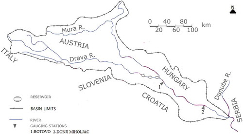
The Drava River is the most important river in Croatia (Tadić et al. 2016). In this study, the sediment discharge characteristics of the lower Drava River, where it crosses the boundary between Slovenia and Croatia, were analysed. Daily discharge and suspended sediment concentration (SSC) from two gauging stations, Botovo and Donji Miholjac, were analysed, as shown in Fig. 1. The Botovo and Donji Miholjac gauging stations are operated by the Croatian Meteorological and Hydrological Service. SSC data were obtained from water samples taken once a day from a single point (close to the riverbed in the water gauging profile). Normally, the sample was taken manually in the morning. The sample was poured through a 0.45-μm filter paper. Sample filtration was done using Munktell filter paper, 320 mm in diameter.

Figure 1. Location maps of the Drava River, with the positions of two gauging stations

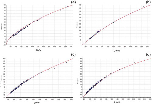
Daily discharge was calculated from hourly values based on hourly measurements of water level (WL). The WL-Q method was used for hourly Q calculations. The defined RK varied over time due to morphological changes in the river bed. Because of this, there are many rating curves to present. For reasons of space, only two RK examples per station – the newest one, and one from 2009 – are provided (see Fig. 2). The main characteristics of the two gauging stations, including distance from the river mouth, basin area, elevation and the available data period are shown in Table 1.

Table 1. Statistics of data used in the present study

Station	Basin area (km^2)	Elevation (meter above sea level)	Quantity	Period of record	Minimum	Maximum	Mean	Coefficient of variation
Botovo	31 038	121.55	Discharge (m^3/s)	1987–2017	103.00	2322.00	474.75	0.49
			Sediment load (ton/day)	1987–2017	0.54	66,199.75	836.75	1.89
DonjiMiholjac	37 142	88.57	Discharge (m^3/s)	1987–2017	175.00	2166.00	509.55	0.44
			Sediment load (ton/day)	1987–2017	0.18	22,788.86	727.98	1.62

Figure 2. WL-Q examples for each station: (a) Botovo 2009, (b) Botovo 2017–2019, (c) Donji Miholjac 2009, and (d) Donji Miholjac 2017–2019 (Zhu et al. 2019)

Varaždin, Čakovec and Dubrava are the three major hydroelectric power plants constructed in the lower Drava River, with a mean power generation capacity of around 475, 400, 385 GWh/year, respectively. Figure 3 presents the daily SSC and Q time series for the two gauging stations. As the figure shows, the Q values for the two stations generally follow the same temporal pattern, with Botovo station having higher extreme values in the flood season. The difference in the annual mean value of Q between the two stations is small since there are no large tributaries between Botovo and Donji Miholjac (Table 1). Bankfull discharges of 2345 m³/s and 2048 m³/s, respectively, were observed during September 2014 floods at Botovo and Donji Miholjac gauging sites (mvodostaji.voda.hr). Donji Miholjac station is nearly 150 km downstream of Botovo. SSC data was converted into sediment load (S) data by combining it with discharge data in the present study.

Figure 3. Flowchart presenting the computation of effective discharge using the standard iterative approach

3 Methodology

Effective discharge was computed at the Botovo and Donji Miholjac stations of the Drava River to determine the discharge transporting maximum sediment load over a period of time. Since the concept of effective discharge involves an analysis of both frequency and magnitude of discharge, it is also known as magnitude frequency analysis of sediment transport. In this regard, the entire range of discharge occurring over a period of time at the gauging station was divided into a number of classes, and the frequency of each class was determined. The average sediment load transported by each class was also determined. The number of classes were determined iteratively using the procedure outlined in the flowchart (Fig. 3). Once the number of classes is determined, effective discharge is determined as the class transporting maximum sediment load as shown in Fig. 3.

Another approach to estimate the effective discharge is to use analytical expressions based on various frequency distributions. Sediment transport in rivers is mainly governed by a sediment rating curve, generally expressed as

(1) $S=\mathrm{a}{\mathrm{Q}}^{\mathrm{b}}$(1)

where S = sediment load (t/d) and Q = discharge (m³/s); a and b are regression coefficients.

If F is the frequency of occurrence of a discharge event, then its effectiveness (E) in sediment transport can be expressed as

(2) $E=SF$(2)

For maximum effectiveness or effective discharge identification,

(3) $\frac{\mathrm{\partial }\mathrm{E}}{\mathrm{\partial }\mathrm{Q}}=0$(3)

Depending on the frequency distribution of the discharge series, the effective discharge (Q_e) may be computed.

For a normal distribution (Goodwin 2004),

(4) $Q_e=0.5(\mu +\sqrt{{\mu }^2+4b{\sigma }^2}$(4)

where $\mu =$ average daily discharge; $\sigma$ = standard deviation of discharge and b = regression coefficient of sediment rating curve.

For a lognormal two-parameter (2P) distribution (Goodwin 2004),

(5) $Q_e=e^{\left({\mu }_y+\left(b-1\right){\sigma }_y^2\right)}$(5)

where ${\mu }_y$ = average of log-transformed discharge data and ${\sigma }_y$ = standard deviation of log-transformed discharge data.

For a lognormal three-parameter (3P) distribution (Goodwin 2004),

(6) ${\mu }_{\mathrm{\Psi }}+\left(b-\left(1+\frac{b\gamma }{Q_e}\right)\right){\sigma }_{\mathrm{\Psi }}^2-ln\left(Q_e-\gamma \right)=0$(6)

where ${\mu }_{\mathrm{\Psi }}$ = average of shifted log-transformed discharge data and σ_Ψ = standard deviation of log-transformed discharge data.

For a gamma distribution (Goodwin 2004),

(7) $Q_e=\beta \left(b+\alpha -1\right)$(7)

where $\alpha$ and $\beta$ are shape and threshold parameters of the gamma distribution.

To estimate effective discharge analytically, sediment rating curves were established based on the least squares method using a generalized reduced gradient (GRG) solver at both Botovo and Donji Miholjac gauging stations. The normal, lognormal (2P), lognormal (3P) and gamma frequency distributions were fitted to daily discharge data for both gauging stations to estimate the parameters required to calculate effective discharge analytically. Once the rating curve parameter and the frequency distribution parameters are determined, analytically effective discharge can easily be calculated using Microsoft Excel based on Equations (4)(4) $Q_e=0.5(\mu +\sqrt{{\mu }^2+4b{\sigma }^2}$(4) , (5(5) $Q_e=e^{\left({\mu }_y+\left(b-1\right){\sigma }_y^2\right)}$(5) ) and (7(7) $Q_e=\beta \left(b+\alpha -1\right)$(7) ). Further, to estimate effective discharge using Equation (6)(6) ${\mu }_{\mathrm{\Psi }}+\left(b-\left(1+\frac{b\gamma }{Q_e}\right)\right){\sigma }_{\mathrm{\Psi }}^2-ln\left(Q_e-\gamma \right)=0$(6) , a (lognormal (3P)) distribution GRG solver was used. Details on the GRG solver can be found in Barati (2013); Muzzammil et al. (2015); Muzzammil et al. (2018); Pandey et al. (2018); Zakwan (2018) and Zakwan (2020).

Apart from the effective discharge, factor load discharge (f-load discharge or Q_f) was also estimated. The generalized expression for calculating Q_f is expressed as follows (Vogel et al. 2003):

(8) $f=1-\mathrm{\Phi }\left[\frac{ln{Q}_f-{\mu }_y-b{\sigma }_y^2}{{\sigma }_y}\right]$(8)

where $\mathrm{\Phi }=$ cumulative distribution function for a standard normal variable and f = fraction of load.

Half load discharge $(Q_{0.5})$ is a special case of f-load discharge, below or above which 50% of the long-term sediment load is transported. The explicit expression for $Q_{0.5}$ can be obtained by putting f = 0.5 in Equation (8)(8) $f=1-\mathrm{\Phi }\left[\frac{ln{Q}_f-{\mu }_y-b{\sigma }_y^2}{{\sigma }_y}\right]$(8) , which yields (Vogel et al. 2003):

(9) $Q_{0.5}=e^{\left({\mu }_y+b{\sigma }_y^2\right)}$(9)

Different frequency distributions were fitted to the annual maximum discharge time series to identify the best-fit distribution. Anderson-Darling (A-D) and Kolmogorov-Smirnov (K-S) tests were employed to ascertain the best-fit distribution using Easyfit 5.6 software. For fitting different frequency distributions, the annual maximum time series is entered into the Easyfit spreadsheet. Then the fit option available in the graphical user interface is clicked. Upon clicking this option the distribution fitting results will pop up, whereupon the user can determine the distribution parameters and goodness of fit by clicking the summary and goodness of fit tabs, respectively. More details on frequency distribution and goodness of fit can be found in Haddad and Rahman (2011) and Hamed and Rao (2019).

Further, discharges of 1.5, 2, 25, 50 and 100 years were estimated using time series of annual maximum discharge, based on the Gumbel distribution given by Equation (10)(10) $Q_T=\bar{Q}+K\sigma$(10) (Subramanya 2008):

(10) $Q_T=\bar{Q}+K\sigma$(10)

where $Q_T$ = discharge of T years return interval; $\bar{Q}$ = annual average maximum discharge K = frequency factor; and $\sigma =$standard deviation of annual maximum discharge series.

The confidence limit was calculated as follows (Subramanya 2008):

(11) $Q_{\mathrm{U}/\mathrm{L}}=Q_T\pm f\left(c\right)S_e$(11)

(12) $S_e=B\frac{\sigma }{\sqrt{N}}$(12)

(13) $B={\left(1+1.3K+1.1K^2\right)}^{0.5}$(13)

where $f\left(c\right)$ = function of confidence probability ($f\left(c\right)$ = 1.96 at 95% confidence level); $S_e$ = probable error; and N = sample size of annual maximum time series.

4 Results and discussion

4.1 Seasonality of flow

Flow in many rivers is highly seasonal in nature, and the major portion of discharge in such rivers is observed during only a few months of the year while the river maintains negligible discharge for most of the year. Since the concept of effective discharge is based on the magnitude as well as the frequency of flow, the role of seasonality of flow becomes important. In many cases where low flows prevail for most of the year, the frequency of low flows becomes so high that it overrides moderate- or high-magnitude flows in term of sediment transport, despite having a negligible role in channel formation. To overcome such effects, Ashmore and Day (1988) and Zakwan et al. (2018) used only the sediment discharge data of the monsoon period for computation of effective discharge. In this regard, seasonal variation of discharge and suspended sediment load (SSL) was studied at the two stations and is shown in Fig. 4.

Figure 4. Monthly average discharges at (a) Botovo and (b) Donji Miholjac and monthly average sediment load at (c) Botovo and (d) Donji Miholjac

A perusal of Fig. 4 reveals that at both stations, Botovo and Donji Miholjac, there is no significant monthly variation in discharge or SSL. However, as compared to discharge, monthly variation in sediment load is more pronounced in SSL, as evident from Fig. 4(c) and (d). Typically, SSL is far below the average load for the months of December, January and February at both gauging sites, hinting at the low sediment transport potential of low flows as observed during these months. The maximum average discharge and SSL are observed in May and June, which may be attributed to high rainfall during these months and the snowmelt received from the headwater part of the Drava catchment in Austria (Bonacci and Oskoruš 2010). The annual average discharge was 475 and 509 m³/s, while the average monthly discharge in May was 604 and 611 m³/s, at Botovo and Donji Miholjac, respectively. Since there is no significant difference in maximum monthly discharge and annual average discharge, discharge and sediment data for all months were considered in the computation of effective discharge.

4.2 Characteristics of effective transport curve

Effective suspended sediment transport histograms for the Botovo and Donji Miholjac stations are shown in Fig. 5. Figure 5 represents the sediment transport capacity of discharges experienced by the river at the two stations. The shape or the nature of the effective transport histogram or curve demonstrates the impacts that different discharges have on the river channel shape. Working with the concept of effective discharge, scientists have observed the diverse nature of effective transport curves. While most researchers observed unimodal effective sediment transport curves (Wolman and Miller 1960, Pickup and Warner 1976, Quader et al. 2008, Higgins et al. 2016), Ashmore and Day (1988) reported three categories of effective transport curves on the Saskatchewan River, Canada. Ashmore and Day (1988) observed effective transport curves with a single distinguished peak, with multiple peaks, without any noticeable peaks or with a broad flat peak. López-Tarazón and Batalla (2014) computed the effective discharge for the Isabena River and observed two peaks in the effective suspended sediment transport curves. On the Isabena River the primary peak of the transport curve was observed for low discharges while the secondary peak corresponded to significantly higher discharges. Dumitriu (2018) reported very noisy sediment load histograms with multiple peaks for the Trotus River in Romania. Zakwan et al. (2018) observed a single sharp peak for most stations on the Ganga River; however, no distinct peak was observed at Varanasi station.

Figure 5. Histograms of effective suspended sediment transport at (a) Botovo and (b) Donji Miholjac

In the present case, Fig. 5 clearly demonstrates the unimodal nature of the transport curve. It may be observed at both stations that high discharges are too infrequent to exert a noticeable impact on the sediment transport regime of the river. On the other hand, extremely low discharges have very low potential to contribute to sediment transport, as is evident from the left side of the transport curves (Fig. 5). Discharges of magnitude around the annual average discharge (475 and 509 m³/s for Botovo and Donji Miholjac, respectively) contribute significantly towards suspended sediment transport in the lower Drava River. Based on the effective suspended sediment transport histograms, it may be concluded that maximum sediment in the lower Drava River is transported by frequently occurring discharges which are approximately equal to the annual average daily discharge.

Figure 6 shows the frequency of occurrence (%) for each discharge class interval. the figure clearly shows that the discharges with magnitude around that of the annual average discharge are the most frequently occurring discharges, whereas discharges with magnitude above 2000 m³/s are most infrequent at both stations. Typically, at Botovo, the number of discharge events in the class interval 630–715 m³/s was observed to be 760, and its average sediment transport capacity was 1527 ton. On the other hand, the sediment transport capacity of discharge class 2180–2265 m³/s (close to bankfull discharge) is around 5275 ton; however, discharges of this range occurred only thrice, and therefore, the contribution of discharge class 2180–2265 m³/s towards overall sediment transport is negligible (as shown in Fig. 5(a)). Similarly, at Donji Miholjac, the number of discharge events in the class interval 490–530 m³/s was observed to be 1354, and its average sediment transport capacity was 725 ton. On the other hand, the sediment transport capacity of discharge class 2090–2170 m³/s (close to bankfull discharge) is around 2700 ton; however, discharges of this range occurred only twice, and therefore, the contribution of discharge class 2090–2170 m³/s towards overall sediment transport is negligible (as shown in Fig. 5(b)).

Figure 6. Frequency of different discharge classes at (a) Botovo and (b) Donji Miholjac

Effective discharge (673 and 530 m³/s at Botovo and Donji Miholjac, respectively) is much smaller than bankfull discharge (2345 and 2048 m³/s at Botovo and Donji Miholjac, respectively) in the lower Drava River. The high ratio of bankfull discharge and effective discharge signifies channel incision. Deep incision in the lower Drava River has also been reported by Lóczy (2018) and Burián et al. (2019), confirming the present finding.

4.3 Impact of data aggregation on effective discharge

Recently, Zakwan et al. (2018) analysed the impact of data aggregation on effective discharge. Working on similar grounds, the impact of data aggregation on effective discharge computation was analysed for the present dataset also. The daily suspended sediment and discharge data were converted to 10-d average and monthly average data. Thereafter, effective discharge was calculated based on 10-d average and monthly average data for both Botovo and Donji Miholjac stations in the Drava River. The effective discharge was calculated for 10-d average and monthly average data as shown in Table 2.

Table 2. Effect of data aggregation on effective discharge

Station	Qe (Daily)	Qe (10-d average)		Qe (Monthly average)
	(m^3/s)	(m^3/s)	% difference from daily Qe	(m^3/s)	% difference from daily Qe
Botovo	673	638	5.20	621	7.23
Donji Miholjac	530	538	1.51	745	40.57

It may be observed that the effective discharge calculated based on 10-d average and monthly average data is significantly different from that calculated from daily data. At the Donji Miholjac station, the effective discharge obtained from daily data is 530 m³/s, while the effective discharge from monthly data was calculated as 745 m³/s – about 40% higher. Earlier, Zakwan et al. (2018) reported that effective discharge computation is marginally affected by data aggregation on large rivers like the Ganga. The discharge in the Drava River is much smaller than that in the Ganga River. In the case of large rivers (such as Ganga River), there is little difference between daily and 10-d average discharge (Roy and Sinha 2014, Zakwan et al. 2018). However, a significant difference was observed here among daily, 10-d average and monthly average discharge, leading to differences in effective discharge in the present case. In this regard, it would be appropriate to calculate effective discharge based on daily discharge data. Further, it may also be observed that a change in the frequency of data collection may lead to overestimation or underestimation of effective discharge.

4.4 Analytical estimates of effective discharge

Figure 7 presents the sediment discharge rating curves for the Botovo and Donji Miholjac stations. The correlation coefficient and coefficient of determination were 0.85 and 0.70, respectively, for the sediment rating curve developed for Botovo, while at Donji Miholjac the correlation coefficient and coefficient of determination were 0.82 and 0.68, respectively. As can be seen in Fig. 7, large scatter exists in the sediment discharge data. The scatter is more pronounced at the Donji Miholjac gauging station. Discharge sediment ratings are affected by a number of factors apart from discharge, such as velocity, precipitation, shear stress, human intervention, bed form geometry and the friction factor (Asselman 2000). As a result, a large scatter in discharge sediment ratings has been observed in many rivers of the world (Asselman 2000, Zakwan et al. 2018, Zhu et al. 2019).

Figure 7. Sediment discharge rating curves at (a) Botovo and (b) Donji Miholjac

Normal, lognormal (2P), lognormal (3P) and gamma frequency distributions were fitted to the daily discharge data for both stations. Frequency distribution parameters for both stations are reported in Table 3. Using the rating curve parameter “b” along with frequency distribution parameters in Equations (4(4) $Q_e=0.5(\mu +\sqrt{{\mu }^2+4b{\sigma }^2}$(4) –7(7) $Q_e=\beta \left(b+\alpha -1\right)$(7) ), analytical estimates of effective discharge were obtained based on normal, lognormal (2P), lognormal (3P) and gamma frequency distributions. Analytical estimates of effective discharge at the two stations are given in Table 4. These were found to be in good agreement with the effective discharge obtained from the effective discharge histograms. It was observed that Equations (4(4) $Q_e=0.5(\mu +\sqrt{{\mu }^2+4b{\sigma }^2}$(4) –7(7) $Q_e=\beta \left(b+\alpha -1\right)$(7) ) are independent of the sediment rating curve coefficient “a”; therefore, if the bed load is assumed to represent a certain proportion of the total load, the same analytical estimates of effective discharge would work for total load transport. However, as the sediment rating curves often under- or overestimate the sediment load (Ferguson 1986, Muzzammil et al. 2018, Zakwan 2018, Zakwan et al. 2018), for reliable estimation of effective discharge the observed sediment load data should be used.

Table 3. Daily discharge frequency distribution parameters

Station	Distribution parameters
	Normal	Lognormal (2P)	Lognormal (3P)	Gamma
Botovo	σ = 231.09 µ = 474.75	σy = 0.44 µy = 6.06	σΨ = 0.54 µΨ = 5.85 γ = 72.17	α = 5.12 β = 92.78
Donji Miholjac	σ = 224.44 µ = 509.55	σy = 0.40 µy = 6.15	σΨ = 0.56 µΨ = 5.79, γ = 124.91	α = 6.10 β = 83.48

Table 4. Analytical estimates of effective discharge

Station	Effective discharge (m^3/s)
	Normal	Lognormal (2P)	Lognormal (3P)	Gamma
Botovo	682	592	584	483
Donji Miholjac	669	561	525	515

4.5 Estimation of f-load discharge

Q_f provides the estimate of discharge above which f fraction of long-term discharge is transported. In this regard, discharges above which 0.9–0.1 fraction of sediment load are transported were calculated using Equation (8)(8) $f=1-\mathrm{\Phi }\left[\frac{ln{Q}_f-{\mu }_y-b{\sigma }_y^2}{{\sigma }_y}\right]$(8) for both stations and are reported in Table 5. Half load discharge (Q_0.5), representing discharge above and below which 50% of the load is transported, was also estimated. In the case of Q_0.5 Equation (8)(8) $f=1-\mathrm{\Phi }\left[\frac{ln{Q}_f-{\mu }_y-b{\sigma }_y^2}{{\sigma }_y}\right]$(8) turns into Equation (9)(9) $Q_{0.5}=e^{\left({\mu }_y+b{\sigma }_y^2\right)}$(9) , equalizing it to the analytical estimate of effective discharge proposed by Nash (1994). It was observed that the discharge above which a certain fraction of sediment load is transported is higher at the Botovo station as compared to the Donji Miholjac station.

Table 5. Fraction load discharge at Botovo and Donji Miholjac

Fraction (f)	${\mathit{Q}}_{\mathit{f}}$ (Fraction load discharge) (m^3/s)
	Botovo	Donji Miholjac
0.1	925.33	813.41
0.2	847.81	756.44
0.3	796.92	718.56
0.4	755.99	687.79
0.5	719.26	659.95
0.6	684.32	633.23
0.7	649.17	606.12
0.8	610.21	575.76
0.9	559.09	535.44

Figure 8 represents the sediment balance between the two stations based on SSL. The sediment balance was calculated as the difference in SSL between the upstream and the downstream station and is presented in Fig. 8. However, Fig. 8 does not represent any constant erosion/deposition in the reach.

Figure 8. Suspended sediment balance between the two stations

4.6 Discharges of specific return interval

Many researchers have reported that effective discharge or discharge transporting maximum sediment load could be approximated by discharges of specific return intervals, such as discharges of a 2-year or 1.5-year return interval in an annual maximum time series. To investigate the relationship between effective discharge and discharges of specific return intervals, frequency distributions were fitted to maximum discharge time series. Commonly used frequency distributions were fitted to annual maximum time series, and best-fit distributions were selected based on A-D and K-S tests. Tables 6 and 7 show the goodness of fit for annual maximum discharge series at the Botovo and Donji Miholjac stations, respectively. The lowest values of the A-D and K-S statistics were observed for the Gumbel distribution at both stations; therefore, the Gumbel distribution was identified as the best fit distribution for both stations.

Table 6. Frequency distribution characteristics of maximum discharge series at Botovo

Distribution	Parameters	K-S	A-D
Gamma	α = 11.643 β = 124.84	0.111	0.467
Gumbel	σg = 332.14 µg = 1261.80	0.082	0.261
Lognormal (2P)	σy = 0.28186 µy = 7.2417	0.093	0.314
Lognormal (3P)	σΨ = 0.3129 µΨ = 7.1365 γ = 133.51	0.091	0.293
Normal	σ = 425.98 µ = 1453.6	0.142	1.00

Table 7. Frequency distribution characteristics of maximum discharge series at Donji Miholjac

Distribution	Parameters	K-S	A-D
Gamma	α = 15.075 β = 86.571	0.097	0.452
Gumbel	σg = 262.08 µg = 1153.8	0.079	0.334
Lognormal (2P)	σy = 0.24994 µy = 7.1428	0.086	0.375
Lognormal (3P)	σΨ = 0.23594 µΨ = 7.2003 γ = −72.685	0.085	0.371
Normal	σ = 336.13 µ = 1305	0.119	0.792

Equation (10)(10) $Q_T=\bar{Q}+K\sigma$(10) was used to estimate Q_1.5 and Q₂ based on the Gumbel distribution. Q_1.5 and Q₂ at a 95% confidence level are reported in Table 8. Apart from Q_1.5 and Q₂, Q₂₅, Q₅₀ and Q₁₀₀, important from the point of view of designing important hydraulic structures, spillway capacities and other flood management projects, were also estimated and are reported in Table 8.

Table 8. Discharges of various return intervals based on the Gumbel distribution

Station	Q1.5 (m^3/s)	Q2 (m^3/s)	Q25 (m^3/s)	Q50 (m^3/s)	Q100(m^3/s)
Botovo	1217.16 ± 95.69	1386.92 ± 110.52	2431.92 ± 380.85	2689.85 ± 456.15	2947.36 ± 532.05
Donji Miholjac	1118.55 ± 7.50	1252.50 ± 87.20	2076.61 ± 300.51	2280.20 ± 359.91	2483.79 ± 419.92

4.7 Comparison of different discharge indices

Effective discharge, fraction load discharge and discharge of specific return intervals (Q_1.5 and Q₂) were calculated at both stations. It was observed that Q_1.5 and Q₂ are much higher in magnitude than effective discharge. In fact, Q_1.5 and Q₂ are almost double the effective discharge. Effective discharge is also smaller than half load discharge (Q_0.5) at both stations, which shows that effective discharge transports less than 50% of the total sediment load over the given period of time. Interestingly, the discharge responsible for transporting 90% (Q_0.1) of long-term sediment load at the Botovo (925 m³/s) and Donji Miholjac (813 m³/s) stations is much lower than the annual average maximum discharges (1455 and 1305 m³/s at Botovo and Donji Miholjac stations, respectively).

The return interval of Q_0.1 on the annual maximum discharge time series based on Equation (10)(10) $Q_T=\bar{Q}+K\sigma$(10) turns out to be 1.10 years and 1.05 years at Botovo and Donji Miholjac stations, respectively. The return interval of Q_0.1 suggests that 90% of the long-term sediment load at these stations is transported by discharge expected to occur annually, which further reinforces our finding that frequently occurring discharges in the lower Drava River basin are responsible for transporting a major fraction of SSL. Q_0.1 is approximately 1.37 and 1.53 times Q_e at Botovo and Donji Miholjac, respectively, and obviously the return interval of effective discharge is less than 1 year.

Lastly, the total SSL over the period of time can be calculated as the sum of the sediment load transported by each class, as shown in Fig. 5. The f-load discharges, as given in Table 5, represent discharge above which f-fraction of sediment load is transported. These quantities provide important guidelines for the stakeholders of hydropower projects. Reservoir sedimentation is the most common problem faced by hydropower projects. High rates of sediment deposition, especially near the dam, resulting from reduced flow velocity may potentially reduce the storage capacity. High sediment concentration may also be harmful for the machinery of hydropower plants.

5 Conclusion

The present study investigates the flow and sediment transport characteristics of two gauging stations, Botovo and Donji Miholjac, on the lower Drava River. Based on the present analysis, it is concluded that (i) discharge and sediment load do not present significant seasonality in the lower Drava River; (ii) effective discharge or discharge responsible for maximum sediment transport is a frequent event in the Drava River, with a recurrence interval of less than 1 year. Extreme events are too infrequent to transport a sizable amount of sediment load; (iii) unlike in the case of large rivers, the effective discharge computation is significantly affected by data aggregation as observed in the present study. Significant differences in effective discharge computed from daily, 10-d average and monthly average data were observed; (iv) effective discharge was also estimated analytically based on normal, lognormal (2P), lognormal (3P) and gamma frequency distributions, and these were in good agreement with the effective discharge computed from sediment load histograms; (v) discharge with return intervals of 1.5 years and 2 years is almost double the effective discharge and, therefore, cannot be used as an approximation of effective discharge; (vi) the magnitude of effective discharge is close to that of the average daily discharge, which is expected to be much lower than bankfull discharge, thereby signifying incised channels; (vii) more than 90% of the long-term sediment load is transported by discharges with a return interval close to 1 year, as revealed by the f-load computation; and (viii) estimates of effective discharge and f-load discharge can be very useful in the design of hydraulic structures and reservoirs and in the operation of hydropower projects.

Disclosure statement

No potential conflict of interest was reported by the authors.

References

- Andrews, E.D., 1980. Effective and bankfull discharge of streams in the Yampa River basin, Colorado and Wyoming. Journal of Hydrology, 46 (3–4), 311–330. doi:https://doi.org/10.1016/0022-1694(80)90084-0
- Andrews, E.D. and Nankervis, J.M., 1995. Effective discharge and the design of channel maintenance flows for Gravel Bed Rivers. In: J.E. Costa, et al., eds. Natural and anthropogenic influences in fluvial geomorphology. Washington, USA: American Geophysical Union, 151–164.
- Ashmore, P.E. and Day, T.J., 1988. Effective discharge for suspended sediment transport in streams of the Saskatchewan River basin. Water Resources Research, 24 (6), 864–870. doi:https://doi.org/10.1029/WR024i006p00864
- Asselman, N.E.M., 2000. Fitting and interpretation of sediment rating curves. Journal of Hydrology, 234 (3–4), 228–248. doi:https://doi.org/10.1016/S0022-1694(00)00253-5
- Barati, R., 2013. Application of excel solver for parameter estimation of the nonlinear Muskingum models. KSCE Journal of Civil Engineering, 17 (5), 1139–1148. doi:https://doi.org/10.1007/s12205-013-0037-2
- Biedenharn, D.S., et al., 2000. Effective discharge calculation: a practical guide. Technical report. Vicksburg, MS: U.S. Army Engineer Research and Development Center, 1–48.
- Biedenharn, D.S., Little, C.D., and Thorne, C.R., 1987. Magnitude and frequency analysis in large rivers. In: Proceeding of Hydraulic Engineering. Vicksburg, USA: ASCE, 782–787.
- Biedenharn, D.S. and Thorne, C.R., 1994. Magnitude-frequency analysis of sediment transport in the lower Mississippi river. Regulated Rivers: Research & Management, 9 (4), 237–251. doi:https://doi.org/10.1002/rrr.3450090405
- Bonacci, O. and Oskoruš, D., 2010. The changes in the lower Drava River water level, discharge and suspended sediment regime. Environmental Earth Sciences, 59 (8), 1661–1670. doi:https://doi.org/10.1007/s12665-009-0148-8
- Burián, A., Horváth, G., and Márk, L., 2019. Channel incision along the lower Drava. In: D. Lóczy, ed. The Drava River. Pécs, Hungary: Springer, 139–156.
- Dean, D.J., et al., 2016. Sediment supply versus local hydraulic controls on sediment transport and storage in a river with large sediment loads. Journal of Geophysical Research: Earth Surface, 121 (1), 82–110.
- Downs, P.W., Skinner, K., and Soar, P.J., 1999. Muddy waters: issues in assessing the impact of in-stream structures for river restoration. In: I. Rutherford and R. Bartley, eds. Second Australian stream management conference: the challenge of rehabilitating Australia’s streams, Adelaide, South Australia. Clayton, Australia: Cooperative Research Centre for Catchment Hydrology, Monash University, 211–217.
- Dumitriu, D., 2018. Sub-bankfull flow frequency versus magnitude of flood events in outlining effective discharges. Case study: Trotuș River (Romania). Water, 10 (10), 1292. doi:https://doi.org/10.3390/w10101292
- Ferguson, R.I., 1986. River loads underestimated by rating curves. Water Resources Research, 22 (1), 74–76. doi:https://doi.org/10.1029/WR022i001p00074
- Goodwin, P., 2004. Analytical solutions for estimating effective discharge. Journal of Hydraulic Engineering, 130 (8), 729–738. doi:https://doi.org/10.1061/(ASCE)0733-9429(2004)130:8(729)
- Guo, Y., Quader, A., and Stedinger, J.R., 2016. Analytical estimation of geomorphic discharge indices for small intermittent streams. Journal of Hydrologic Engineering, 21 (7), 04016015. doi:https://doi.org/10.1061/(ASCE)HE.1943-5584.0001368
- Haddad, K. and Rahman, A., 2011. Selection of the best fit flood frequency distribution and parameter estimation procedure: a case study for Tasmania in Australia. Stochastic Environmental Research and Risk Assessment, 25 (3), 415–428. doi:https://doi.org/10.1007/s00477-010-0412-1
- Hamed, K. and Rao, A.R., eds., 2019. Flood frequency analysis. Florida, FL: CRC press.
- Hassan, M.A., et al., 2014. Effective discharge in small formerly glaciated mountain streams of British Columbia: limitations and implications. Water Resources Research, 50 (5), 4440–4458. doi:https://doi.org/10.1002/2013WR014529
- Higgins, A., et al., 2016. Suspended sediment transport in the Magdalena River (Colombia, South America): hydrologic regime, rating parameters and effective discharge variability. International Journal of Sediment Research, 31 (1), 25–35. doi:https://doi.org/10.1016/j.ijsrc.2015.04.003
- Hudson, P.F. and Mossa, J., 1997. Suspended sediment transport effectiveness of three large impounded rivers, U.S. Gulf Coastal Plain. Environmental Geology, 32 (4), 263–273. doi:https://doi.org/10.1007/s002540050216
- Lóczy, D., ed., 2018. The Drava River: environmental problems and solutions. Pécs, Hungary: Springer.
- López-Tarazón, J.A. and Batalla, R.J., 2014. Dominant discharges for suspended sediment transport in a highly active Pyrenean river. Journal of Soils and Sediments, 14 (12), 2019–2030. doi:https://doi.org/10.1007/s11368-014-0961-x
- Lyons, J.K., Pucherelli, M.J., and Clark, R.C., 1992. Sediment transport and channel characteristics of a sand-bed portion of the Green River below Flaming Gorge Dam, Utah, USA. Regulated Rivers: Research & Management, 7 (3), 219–232. doi:https://doi.org/10.1002/rrr.3450070302
- Malik, A., et al., 2020. Support vector regression optimized by meta-heuristic algorithms for daily streamflow prediction. Stochastic Environmental Research and Risk Assessment, 34 (11), 1755–1773. doi:https://doi.org/10.1007/s00477-020-01874-1
- McKay, S.K., Freeman, M.C., and Covich, A.P., 2016. Application of effective discharge analysis to environmental flow decision-making. Environmental Management, 57 (6), 1153–1165. http://mvodostaji.voda.hr/Home/PregledVodostajaPostaje?
- Muzzammil, M., Alam, J., and Zakwan, M., 2015. An optimization technique for estimation of rating curve parameters. In: National symposium on hydrology. New Delhi, 234–240.
- Muzzammil, M., Alam, J., and Zakwan, M., 2018. A spreadsheet approach for prediction of rating curve parameters. In: V.P Singh, et al., eds. Hydrologic modeling. Singapore: Springer, 525–533. doi:https://doi.org/10.1007/978-981-10-5801-1_36
- Nash, D.B., 1994. Effective sediment-transporting discharge from magnitude–frequency analysis. The Journal of Geology, 102 (1), 79–95. doi:https://doi.org/10.1086/629649
- Niazkar, M. and Zakwan, M., 2021. Assessment of artificial intelligence models for developing single-value and loop rating curves. Complexity, 2021, 1–21. doi:https://doi.org/10.1155/2021/6627011
- Pandey, M., et al., 2018. Multiple linear regression and genetic algorithm approaches to predict temporal scour depth near circular pier in non-cohesive sediment. ISH Journal of Hydraulic Engineering, 26 (1), 96–103. doi:https://doi.org/10.1080/09715010.2018.1457455
- Pickup, G. and Warner, R.F., 1976. Effects of hydrologic regime on magnitude and frequency of dominant discharge. Journal of Hydrology, 29 (1–2), 51–75. doi:https://doi.org/10.1016/0022-1694(76)90005-6
- Powell, G.E., Mecklenburg, D., and Ward, A., 2006. Evaluating channel-forming discharges: a study of large rivers in Ohio. Transactions of the ASABE, 49 (1), 35–46. doi:https://doi.org/10.13031/2013.20242
- Quader, A. and Guo, Y., 2009. Relative importance of hydrological and sediment-transport characteristics affecting effective discharge of small urban streams in southern Ontario. Journal of Hydrologic Engineering, 14 (7), 698–710. doi:https://doi.org/10.1061/(ASCE)HE.1943-5584.0000042
- Quader, A., Guo, Y.P., and Stedinger, J.R., 2008. Analytical estimation of effective discharge for small southern Ontario streams. Canadian Journal of Civil Engineering, 35 (12), 1414–1426. doi:https://doi.org/10.1139/L08-088
- Roy, N.G. and Sinha, R., 2014. Effective discharge for suspended sediment transport of the Ganga River and its geomorphic implication. Geomorphology, 227, 18–30. doi:https://doi.org/10.1016/j.geomorph.2014.04.029
- Subramanya, K., 2008. Engineering hydrology. 3rd ed. New Delhi: Tata McGraw-Hill, 261–262.
- Tadić, L., Bonacci, O., and Dadić, T., 2016. Analysis of the Drava and Danube rivers floods in Osijek (Croatia) and possibility of their coincidence. Environmental Earth Sciences, 75 (18), 1238. doi:https://doi.org/10.1007/s12665-016-6052-0
- Tamás, E.A., 2019. Sediment transport of the Drava River. In: D. Lóczy, ed. The Drava River. Cham, Hungary: Springer, 91–103.
- Tilleard, J., 1999. Effective discharge as an aid to river rehabilitation. In: I. Rutherford and R. Bartley, eds. Second Australian stream management conference: the challenge of rehabilitating Australia’s streams, Adelaide, South Australia. Clayton, Australia: Cooperative Research Centre for Catchment Hydrology, Monash University, 629–635.
- Vercruysse, K., Grabowski, R.C., and Rickson, R.J., 2017. Suspended sediment transport dynamics in rivers: multi-scale drivers of temporal variation. Earth-Science Reviews, 166, 38–52. doi:https://doi.org/10.1016/j.earscirev.2016.12.016
- Vogel, R.M., Stedinger, J.R., and Hooper, R.P., 2003. Discharge indices for water quality loads. Water Resources Research, 39 (10). doi:https://doi.org/10.1029/2002WR001872
- Wolman, M.G. and Miller, J.P., 1960. Magnitude and frequency of forces in geomorphic processes. The Journal of Geology, 68 (1), 54–74. doi:https://doi.org/10.1086/626637
- Wyżga, B., et al., 2020. Use of high-water marks and effective discharge calculation to optimize the height of bank revetments in an incised river channel. Geomorphology, 356, 107098. doi:https://doi.org/10.1016/j.geomorph.2020.107098
- Zakwan, M., 2018. Spreadsheet-based modelling of hysteresis-affected curves. Applied Water Science, 8 (4), 101–105. doi:https://doi.org/10.1007/s13201-018-0745-3
- Zakwan, M., 2020. Revisiting maximum observed precipitation and discharge envelope curves. International Journal of Hydrology Science and Technology, 10 (3), 221–229. doi:https://doi.org/10.1504/IJHST.2020.107215
- Zakwan, M., Ahmad, Z., and Sharief, S.M.V., 2018. Magnitude-frequency analysis for suspended sediment transport in the Ganga River. Journal of Hydrologic Engineering, 23 (7), 05018013. doi:https://doi.org/10.1061/(ASCE)HE.1943-5584.0001671
- Zetterqvist, L., 1991. Statistical estimation and interpretation of trends in water quality time series. Water Resources Research, 27 (7), 1637–1648. doi:https://doi.org/10.1029/91WR00478
- Zhu, S., Bonacci, O., and Oskoruš, D., 2019. Assessing sediment regime alteration of the lower Drava River. Electronic Journal of the Faculty of Civil Engineering Osijek-e-GFOS, 10 (19), 1–12.