Land cover change induced sediment transport behaviour in a large tropical Mexican catchment

ABSTRACT

The cause–effect relationship and rates of change of suspended sediment dynamics at catchment scales in the tropics remain poorly understood. This study used a chrono-sequence of remotely sensed land use and historical hydrometric data from 1985 to 2001 in three tropical streams of Mexico to analyse the temporal dynamics of land-use change and measured suspended sediment behaviour. The variations in measured suspended sediment concentrations (SSC) were related to land cover change using trend and hysteresis analysis. No statistically significant trends (p > 0.1) at a monthly scale were associated with the historical trajectories of stream sediment fluxes. However, intra-annual hysteresis allowed us to identify the climatic seasonality as a main driver for the discharge-sediment loops and to infer sediment source variations, related to land cover changes over time. The land cover change analysis, combined with statistical tests and hysteresis, was useful to identify temporal and spatial variations in sediment source dynamics.

KEYWORDS:

• land cover change
• suspended sediment
• statistical trends
• hysteresis
• tropical hydrology
• Papaloapan River
• Mexico

Editor S. Archfield ; Associate editor J. Rodrigo-Comino

Introduction

Over the last decade, reforestation efforts worldwide have slowed land cover changes (FAO 2011). However, Latin America and the Caribbean region represent the highest net forest loss in the world, with an annual forest cover change rate of −0.46% between 2000 and 2010, equivalent to more than 3 times the average global rate (−0.13%) for the same period (FAO 2011). In the case of Mexico, the annual forest loss amounts to 0.30%, with up to 1% for primary forests (Blackman et al. 2018).

Both the land use and land cover changes (LULCC) result directly from human intervention (Velázquez et al. 2002, Wohl et al. 2012), and in tropical countries concerns are related to the limited knowledge available about their impacts on soil and water quality at the catchment scale. In the context of Mexico, a typical sequence of conversion from forests to agriculture and pasture and subsequently to urbanization has been observed (Torres-Rojo et al. 2016). Derived impacts from LULCC such as the increase in soil erosion and runoff are critical for environmental management in Mexico, since more than two-thirds of its territory are currently affected by some degree of water erosion and soil loss (Bolaños-González et al. 2016).

Research addressing sediment origin and transport increased recently, based on awareness of the connection between sedimentological and hydrological processes driven by human interventions (Persichillo et al. 2018, Owens 2020, Poeppl et al. 2020) but also due to highlighting the importance of ecosystem services valuation at the catchment scale (Lusardi et al. 2020). In light of potential future adverse consequences of LULCC that cannot be identified by hydrological model parameters alone (Bruijnzeel 2004, Sun et al. 2016), we should also consider the historical trajectory of catchment modifications (Reid 1998, Minella et al. 2017). Hence, studies that contribute to a better understanding of spatial and temporal dynamics of water and sediment fluxes are still needed (Moragoda and Cohen 2020).

It is well known that the land use, the climate regime and the local geology are factors that condition sediment availability at the catchment scale (Douglas and Guyot 2005, Gellis 2013, Sun et al. 2016). More specifically, the study of the discharge (Q) and suspended sediment concentration (SSC) relationship bears information about sources, transport and connectivity characteristics (Lloyd et al. 2016, Zuecco et al. 2016). With long records being available, variability in time and space can be detected (Warrick 2014, Rose et al. 2018) so that future changes can be anticipated and policies for restoration, conservation and management can be implemented (Warrick 2014).

Given the current knowledge gaps in SSC dynamics in tropical catchments driven by LULCC, the main objective of this study is to investigate the temporal suspended sediment dynamics related to land use change in a large tropical catchment in Veracruz, Mexico. The specific objectives were: (1) to develop a chronological sequence of satellite-based land cover change from 1986 to 1998 for three sub-catchments, then (2) to analyse historical long-term discharge and suspended sediment data for trends and hysteresis for each sub-catchment and (3) to relate the discharge-suspended sediment hysteresis and trend analysis to land cover changes over time.

Study area and datasets

The Papaloapan catchment has an area of approximately 46 720 km², draining into the Gulf of Mexico, and constitutes one of the most important hydrological basins in Mexico. The three studied sub-catchments represent 69.4% of the whole catchment (Fig. 1), and their principal physiographic and hydrological characteristics are summarized in Table 1.

Figure 1. Location of the study sub-catchments with topography (upper panel), stream network, monitoring stations and long-term annual rainfall (lower panel)

PAP: Papaloapan sub-catchment; AZU: Tesechoacan sub-catchment; CUA: San Juan sub-catchment.

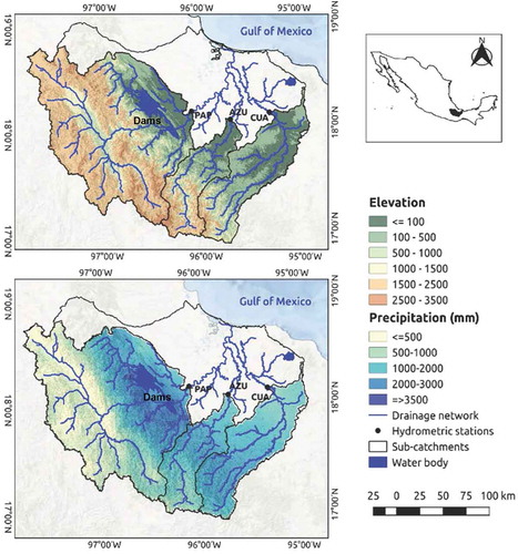
Table 1. Summary of the physical and hydroclimatic characteristics of the study sub-catchments

Gauged sub-catchment	Papaloapan	Tesechoacan	San Juan
Area (km^2)	20685	4665	7077
Altitudinal range (m)	0–3360	0–3401	4–3400
Slope (degrees) [max–min]	18 [0–84]	16 [0–73]	11 [0–72]
Mean annual precipitation (mm)	1485	1918	2101
Mean annual discharge (m^3 s^−1)	562	198	242
Mean annual suspended sediment concentration (mg L^−1)	20.6	8.1	29.3
Mean mass flux (kg s^−1) [max–min]	11.03 [0.12–374]	2.44 [0.04–24]	7.54 [0.15–130]
Stream width at gauging station (m)	238	105	85
Hydrometric station name	Papaloapan (PAP)	Azueta (AZU)	Cuatotolapan (CUA)

The sub-catchments are distributed along an altitudinal gradient from sea level to 3400 m above sea level, with a mean annual rainfall of 1485 mm (Cuervo-Robayo et al. 2014). According to the Köppen climate classification modified by García (2004), the following climate types can be found across the catchment: rainy tropical climate (A) with mean temperatures during the coldest month above 18°C in the lower catchment areas close to sea level; dry climate (BS) with a summer rain regime; and group C with wet temperate and mean temperatures during the coldest months between −3 and 18°C and in the warmer months up to 10°C. The latter climatic group mostly corresponds topographically to the valleys in the mountainous upper catchment. Summer rainfall predominates, with usually dry winters (precipitation on winter <10%). Temperate and tropical forests are concentrated in the mountainous areas, with grasslands and agriculture dominating the lowlands.

The Papaloapan catchment geology is predominantly sedimentary, with metamorphic and igneous materials restricted to the mountainous areas (INEGI 1999). The dominant erosive processes comprise varying degrees of sheet erosion along the catchment, with severe erosion rates focused in the Tesechoacan sub-catchment (AZU) and the San Juan sub-catchment (CUA) lowlands. Gully erosion is restricted to the Papaloapan sub-catchment (PAP) headwaters and small areas in CUA (INEGI 2013).

The Q and SSC records were extracted from the National Database of Surface Waters (CONAGUA 2016), which compiles the historical hydrometric data managed by the National Water Commission (Solís-Alvarado et al. 2015). The hydrological data available are mean hourly, daily, monthly and annual discharges, limnographs and discharge rating curves. Data collected at gauging stations followed established sampling methods (Peters 1998). The suspended sediment sampling was conducted at a water depth of 20 cm, in three points along a transect over the stream using a 1 L glass sampler fixed into an iron frame, with a frequency from twice a week during the dry season to hourly sampling rates in the rainy season. Discharge was estimated from the water height, recorded at least 3 times per day using a discharge rating curve. Despite data gaps (<10%), a common period from 1985 and 2001 was identified for all three catchments.

For the study period, from 1985 to 2001, precipitation data were available from the National Meteorological Service for 58 meteorological stations. Incomplete records were filled with precipitation data from the Climate Hazards Group Infrared Precipitation with Stations (CHIRPS) gridded product, which are estimated from infrared cold cloud duration (CCD) observations (Funk et al. 2015) on a daily basis at a spatial resolution of 0.05°. High correlations between this global precipitation product and field observations were previously reported (Paredes-Trejo et al. 2017, Rivera et al. 2018, Liu et al. 2019).

Land cover was derived from Landsat 5 and 7 satellite imagery with a spatial resolution of 30 m, available from the Google Earth Pro platform (Wuthrich 2006). We used high-quality and cloud-free panchromatic images captured during December of the years 1986, 1993 and 1998.

Methods

Land cover classification

Satellite imagery for land cover classification was processed in QGIS v. 3.4.5 Madeira (QGIS Development Team 2019), using the open-source extension dzetsaka (Karasiak and Perbet 2018, Karasiak 2019). The workflow is illustrated in Fig. 2 and can be summarized as follows: the study area polygon was downloaded and georeferenced for each year. Subsequently, the regions of interest (ROIs) were defined through RGB band combinations and converted into a vector file. The aforementioned ROIs corresponded to land cover and vegetation types defined according to the National Institute of Statistics and Geography. Once the land cover types were clearly defined, the classification was applied to the whole area using a Gaussian mixture model (Fauvel et al. 2015). The model was previously trained with 15% of the total pixels for the baseline year. The validity of the classifications was tested first with a confusion matrix and its accuracy was assessed with both the kappa index of agreement – which assesses the error reduction obtained from the classification versus a random classification – and the overall accuracy index, which identifies the proportion of the total pixels that are correctly classified (Karasiak and Perbet 2018). Finally, pixels were filtered and reclassified to generate the LULCC maps shown in Fig. 3.

Figure 2. The erosion and geological classes of the study catchment

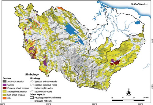
Figure 3. Workflow of land cover and use change analyses

Statistical analysis

The daily discharge and SSC records were first explored with standard pre-processing techniques to visualize data, identify missing values, and remove outliers and potential correlations. The quality-checked data was then averaged to obtain mean monthly values for each sub-catchment, and descriptive statistics were calculated for the mass fluxes.

We chose four non-parametric statistical tests to characterize the sub-catchments’ seasonal sediment transport and the long-term trends as well as to identify possible inflection points in the analysed time series (Xie et al. 2014). First, a Spearman’s rank correlation test was run to measure the level of association as well as its relative direction; this test has been frequently used with seasonal time series (Machiwal and Jha 2012). Subsequently, the Mann-Kendall trend tests in both the original and modified versions (Hamed and Rao 1998) were calculated to assess the relative direction between variables, to explore its trend (Hamed 2016) and then to consider autocorrelation in the data. The Sen’s slope estimation test was applied to quantify monotonic trends. Finally, the Pettitt’s test for single change-point detection was applied to identify gradual or abrupt changes in the time series (Xie et al. 2014).

Q-SSC hysteresis analysis and inference of sediment sources

The Q and SSC relationship was analysed on an intra-annual (mean monthly) and year-to-year scale, using averaged monthly data for a hydrological year defined from 1 February to 31 January. To quantitatively assess the shape, the direction and the magnitude of the hysteretic loops, the hysteresis index (HI) proposed by Zuecco et al. (2016) was used. This index defines eight hysteresis classes, and the shape and direction of the hysteresis loops are conditioned by the mechanisms driving the sediment transport processes (Sun et al. 2016). Thus, the direction according to the sign of HI and the SSC behaviour with respect to the initial state (Fig. 4) summarize the following characteristics:

1. The HI values suggest:

   1. Magnitude: The closer to −1 or +1 the value is, the larger the hysteretic loop.

   2. Direction: A positive sign (+) indicates a clockwise loop (types I, II, V, VI), whereas a negative sign (−) indicates a counterclockwise loop (types III, IV, VII, VIII).

   3. Velocity of source response: The higher the HI value, the larger the differences between the rising and falling limbs, meaning faster SSC variations (Hamshaw et al. 2018).

• (b) The loop direction suggests the distance to sediment sources:

  1. Clockwise: Proximity to sources such as water courses, channel banks and riverbeds or areas near the channel via gully erosion (Collins and Walling 2004, Smith and Dragovich 2009, Sun et al. 2016, Hamshaw et al. 2018, Yang and Lee 2018).

  2. Counterclockwise: Distant sources such as hillslopes, colluvial deposits or upper reaches (Sherriff et al. 2016, Sun et al. 2016, Hamshaw et al. 2018, Yang and Lee 2018).

  3. Figure-eight-shaped pattern: These complex loops (types II, III, VI and VII) are source combinations classified according to the dominant direction of the larger section of the loop (Seeger et al. 2004, Sun et al. 2016, Hamshaw et al. 2018, Yang and Lee 2018).

• (c) The SSC behaviour from the initial state represents the dominant mechanism of mobilization from sources (Regüés et al. 2000):

  1. Increasing: during the dry season discharge acts on nearby sources to supply suspended sediment (types I–IV).

  2. Decreasing: during the dry season, suspended sediment is limited; later, runoff guarantees the sediment supply from surface sources during the rainy season (types V–VIII).

Figure 4. The eight hysteresis classes (after Zuecco et al. 2016) according to the hysteresis index (HI) value signs and the suspended sediment concentration (SSC) increase/decrease from the initial state, to show general directions and shapes. The x-axis displays HI values whereas the y-axis shows SSC values

Based on our study results, following Zuecco et al. (2016) and the work of Seeger et al. (2004), Smith and Dragovich (2009), Gellis (2013), Sherriff et al. (2016), Sun et al. (2016), Hamshaw et al. (2018), Yang and Lee (2018), Table 2 summarizes the principal characteristics for each hysteresis type described here.

Table 2. Summary of the principal characteristics according to each hysteresis type

Type	Shape and direction	Graph	Q-SS travel time (tt) relationship	Distance to sediment sources	Sediment availability	Dominant transport mechanism
I	Ascendant clockwise		Qtt > SStt	Proximal	Mobilization from nearby sediment sources until depletion at the end of the cycle	In-stream transport
II	Ascendant wide clockwise loop followed by shorter counter clockwise loop		Qtt > SStt then Qtt < SStt	Proximal then distal	Supply from nearby sources until exhaustion on rain season then distal sources on the last part of the cycle	In-stream transport
III	Ascendant narrow clockwise loop followed by wider counter clockwise loop		Qtt < SStt then Qtt > SStt	Proximal then distal	Quick flushing of nearby sources with delay of sediment entrance from distal ones, which are dominant on the last part of the hydrological year	In-stream transport
IV	Ascendant counter clockwise		Qtt < SStt	Distal	Basal supply from in stream sources, delay of entrance from far slopes erosion with high sediment availability	In-stream transport
V	Descendant clockwise		Qtt > SStt	Proximal	Nearby rainfall- activated sediment sources, the detachment of surface soil particles reduces as effective rainfall stops	Surface runoff
VI	Descendant wide clockwise loop followed by shorter counter clockwise loop		Qtt > SStt then Qtt < SStt	Proximal then distal	Exhaustion of in stream and nearby sources, then quick supply of sediment transported from distal sources or reaches	Surface runoff
VII	Descendant narrow clockwise loop followed by wider counter clockwise loop		Qtt < SStt then Qtt > SStt	Proximal then distal	Quick flushing of nearby sources then dominance from distal ones during rainy season	Surface runoff
VIII	Descendant counter clockwise		Qtt < SStt	Distal	High availability through surficial erosion in distal sources with lower aggregate stability	Surface runoff

Q: discharge; SS: suspended sediment.

Results and discussion

Remote sensing applied to LULCC detection in the tropics

Most global studies of LULCC use freely available satellite imagery from platforms such as Landsat (Zhu 2017) for scales between catchments (i.e. Pérez-Vega and Ortiz-Pérez 2002, Muñoz-Villers and López-Blanco 2008, Martínez et al. 2009, Twisa and Buchroithner 2019) and whole countries (see Landholm et al. 2019, Phiri et al. 2019, Venkatappa et al. 2019) because of its numerous advantages as long-term imagery records, global coverage and open access (Young et al. 2017).

In Mexico, efforts are being made to standardize historical records of LULCC between diverse governmental agencies, but due to the high territorial heterogeneity, satellite images require intense fieldwork for adequate image classification at (preferably) a high spatial resolution (Bocco et al. 2001, Velázquez et al. 2002). The advances in geospatial and analytical technologies have increased the potential to generate and analyse remote imagery (Konecny 2014, Finer et al. 2018). However, factors such as the image quality as determined by cloud cover, land cover characteristics and the methods used for atmospheric correction and image classification impact on the final product quality (Mas et al. 2004, Zhu and Woodcock 2014). In the tropics, clouds are frequent, therefore radar imagery such as that from Sentinel or online processing platforms such as Google Earth Engine is rapidly increasing in popularity in the form of providing catalogues of pre-processed satellite imagery, geospatial datasets and scientific networking to increase analytical power aimed at detecting land cover changes (Sidhu et al. 2018) or mapping specific cover types such as crop phenological stages (Dineshkumar et al. 2019). Here, we used pre-processed cloud-free composite Landsat images from Google Earth Pro. Moreover, to increase the accuracy of classification, interest in developing new algorithms has increased (Muñoz-Villers and López-Blanco 2008) and new proposals are emerging continually (i.e. Li et al. 2011, Zhu and Woodcock 2014, Vogelmann et al. 2016, Zhu 2017).

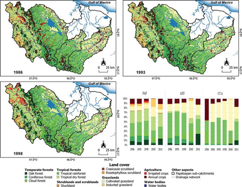
We identified 12 land cover types (excluding water bodies), which were then grouped into five major land cover classes as shown in Table 3. A semi-automatic image classification tool developed for tropical French Guiana (Karasiak 2019) – the dzetsaka algorithm – was used to assess LULCC. The indexes of agreement and accuracy suggested the classifications were acceptable, with kappa values of 59.4, 52.5 and 53.8 for 1986, 1993 and 1998, respectively, and an overall accuracy of 65.9, 60.6 and 61.3 for the same years. The lower spatial resolution (the original work used Satellite for Observation of Earth [SPOT] imagery), the high number of classes (12 in this study) and the differences in floristic composition between vegetation patches of the same type likely contributed to the slightly lower accuracy compared to the 80% obtained in Karasiak’s original study, despite our successive iterations testing different training percentages.

Table 3. Land cover per area (km²) for each period and sub-catchment

Land cover class	Type	PAP			AZU			CUA
		1986	1993	1998	1986	1993	1998	1986	1993	1998
Temperate forests	Oak forest	1726	1230	2292	198	86	175	8	4	10
	Coniferous forest	1962	2775	1643	486	805	391	138	182	94
	Cloud forest	856	425	1470	185	102	528	76	115	223
Tropical forests	Tropical rainforest	5090	5571	5235	2327	2316	2068	3273	3850	3470
	Tropical dry forest	5120	4913	5057	150	126	81	7	2	1
Shrublands and scrublands	Shrubland	244	235	180	11	3	0	3	0	0
	Crasicaule scrubland	42	14	2	0	0	0	0	0	0
	Rosetophyllous scrubland	2	0	0	0	0	0	0	0	0
Grasslands	Cultivated grassland	1858	1838	2069	708	706	979	2773	2326	2878
	Induced grassland	929	1064	753	4	0	0	0	0	0
Agriculture	Irrigated crops	357	88	755	19	0	5	3	0	0
	Rainfed crops	2099	2099	845	512	462	380	717	517	325

PAP: Papaloapan sub-catchment; AZU: Tesechoacan sub-catchment; CUA: San Juan sub-catchment.

Overall, natural vegetation covered more than two-thirds of the area. Thus, tropical forests (on average 16 000 km² across the three sites) were the dominant land cover type in all three sub-catchments, followed by temperate forests (6000 km²), grasslands (6300 km²) and agriculture (3000 km²). The shrublands and scrublands were minor areas (245 km²), susceptible to change as explained further below.

Nonetheless, there were also differences among the three catchments, with tropical rainforest and tropical dry forest being the two most important classes in PAP, covering around 5000 km² each, in contrast to AZU and CUA where tropical dry forest areas were comparatively minimal (120 and 3 km², respectively). Shrublands and scrublands were also more prominent in PAP than in AZU and CUA (surface <5 km² in the latter two). Cultivated grasslands covered around 2600 km² (37% of the total catchment area) of CUA, and induced grasslands (those established after vegetation clearance and repeated burning) were only relevant in PAP at around 1000 km².

Land cover changes between the years 1986, 1993 and 1998 for each sub-catchment (Fig. 3) were estimated from the areal differences in each land cover type and period. The shrublands and scrublands were fully converted into other land covers at AZU and CUA over 12 years, while at PAP about one-third of this land cover type disappeared. The temperate forests increased by 19% at PAP and almost 47% at CUA over the study period. Livestock represented one of the two most important productive activities in the whole Papaloapan River basin (CONAGUA 1989); hence, grassland-covered areas, especially the cultivated ones, tended to increase in all three sub-catchments – by up to 38% in AZU. Over the same period, cultivated areas decreased by 27.5% at AZU, 35% at PAP and 55% at CUA. Tropical forests presented a negative trend at AZU (−13.3%), whereas PAP and CUA showed a small recovery only in 1993.

At the PAP sub-catchment, annual crops in mountain areas were gradually replaced with oak forest from 1986 to 1998. During the same period, irrigated crops were substituted in approximately 75% of the upper streams with coniferous forests and rainforests. In some areas, shrublands and scrublands were converted into irrigated crops until 1998.

The AZU catchment also showed reforestation of former rainfed crop fields in the upper part of the catchment. During the first period, 1986–1993, both oak and cloud forests were reduced by half in size; later (1993–1998) these increased from 4% to 11%. The coniferous forest showed the opposite behaviour, increasing from 10% to 17% and then decreasing to 8%. In contrast, the lower basin rainforests were evidently converted to cultivated grasslands during the 1993–1998 period.

Land cover dynamics in the upper CUA recorded an expansion of cultivated grasslands on former croplands and tropical forest lands, but this was not as drastic a change as for cloud forest areas (from 1% in 1986 to 3% in 1998). In the lower catchment, rainfed crops and cultivated grasslands were abandoned between 1986 and 1993 and were temporarily covered by growing secondary rainforest before these lands were again cleared for cultivated grasslands and cattle farming.

For the Papaloapan sub-catchments, deforestation of between 16 and 30% was reported in the period 1973–1993 with a supervised classification of Landsat imagery (Pérez-Vega and Ortiz-Pérez 2002). Increasing runoff observed in the SSC time series data was attributed to the quantified loss of forested areas.

During the analysed period (1986–1998), pastures and cultures alternated with natural vegetation recovery. This sequence of land exploitation was also verified in the subsequent period (1999–2011). As will be detailed further below, this pattern is relevant for the explanation of the sediment dynamics.

Spatio-temporal suspended sediment behaviour

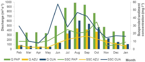
The humid tropics are characterized by high inter-annual and subseasonal variability as well as by intense and pronounced gradients of precipitation (Magaña et al. 2003), which have a significant impact on water and sediment fluxes, proportionally greater than that in temperate zones (Wohl et al. 2012). The hydroclimatic inter-annual regimes were calculated based on 17 years of quality-checked and combined hydrometric records (1985–2001). Hydrological seasonality was defined as: (1) the dry season (from February to May) with no or almost no rain; (2) the rainy season (from June to November) driven by cyclonic events; and (3) the nortes season (from December to March) characterized by intense winter cold fronts coming from the north, generating moderate amounts of precipitation (Appendini et al. 2014, Ojeda et al. 2017).

The peak discharge occurred in August in all three streams. The highest SSC values generally followed the larger discharge flows. However, the highest SSC values were recorded in CUA (29.3 mg L⁻¹) in June at the start of the rainy season, and then in August. AZU exhibited a mean of 8.1 mg L⁻¹, with its maximum SSC recorded in September. PAP mean SSC was 20.6 mg L⁻¹ with the maximum value in October at the end of the rainy season, after a first peak in July (Fig. 5).

Figure 5. The study catchment land cover sequence from 1986, 1993 and 1998, together with a bar chart showing the rate of change per land cover class

Furthermore, the multi-year coupled oceanic–atmospheric phenomenon El Niño Southern Oscillation (ENSO) was responsible for more intense winter rain events (>20%) but decreased average summer precipitation (by 10%) in 1986–1987, 1991–1992, 1992–1993 and 1997–1998 (Magaña et al. 1998, 2003, Bravo-Cabrera et al. 2017). Nevertheless, this influence was not immediately evident in the monthly sediment and discharge time series of the three sub-catchments (Fig. 6).

Figure 6. Inter-annual monthly hydroclimatic regimes for each subcatchment. Q: discharge (left y-axis), SSC: suspended sediment concentration (right y-axis)

PAP: Papaloapan sub-catchment; AZU: Tesechoacan sub-catchment; CUA: San Juan sub-catchment.

The sediment flux rates revealed higher annual values in PAP, with a mean of 347 842 t per year, in contrast to 237 781 t per year in CUA and 76 948 t per year in AZU. However, the annual unit mass flux of PAP and AZU was almost the same, at 16.82 and 16.5 t per km⁻², respectively, despite the much larger catchment area of PAP. The highest suspended sediment delivery, almost twice the values in PAP and AZU, was reported in CUA: 33.6 t per km⁻² anually. These values reflect only the portion of the produced sediment that reached the gauging station. The Spearman’s rank correlation test results of the SSC and Q time series only showed a significant relationship (r = 0.75; SSC = 0.0312Q + 1.97) for AZU. Both PAP and CUA resulted in low correlation coefficients (r = 0.14 and 0.1, respectively). The sediment mass fluxes showed a strong correlation between CUA and AZU (ρ = 0.854), but also detected similar Q-SSC hysteresis loops, that mostly followed the hydrological regime, while the PAP mass flux seemed less related to both CUA (ρ = 0.565) and AZU (ρ = 0.483), with less streamflow regime-related dynamics (Fig. 6).

According to the modified Mann-Kendall trend test (Table 4), with a confidence interval of 0.95, the null hypothesis was accepted for the three sub-catchments since their monotonic negative trends were not significant, as shown by the small Sen’s slope values. Large basins are less reactive to high-frequency external variations (Richards 2002, Peña-Arancibia et al. 2019), which also conforms with the “buffer” effect exerted by the rapid secondary regrowth typical of tropical forests (Bruijnzeel 2004). Such forest recovery reduced the magnitude of LULCC impact on the hydrological variables. However, the only significant inflection point detected for PAP, in September 1987 (Pettit’s test p value = 0.002), was consistent with the historical records. Prior to reservoir operations (1982–1984) the mean sediment flux in PAP was around 21 Mt per year, which after the Cerro de Oro dam operation began in 1988 was reduced by two orders of magnitude. The suggested inflection points for the other sub-catchments (Fig. 7) were December 1999 at AZU (p value = 0.266) and October 1994 at CUA (p value = 0.147), but these were not statistically significant and were more related to the overall hydroclimatic variability.

Table 4. Statistical trend tests applied to the sediment mass flux time series

		PAP	AZU	CUA
Mann-Kendall test	Original Z	−2.52	−1.09	−1.79
	Original p value	0.01	0.28	0.07
	Original variance	950 260.3	949 999.7	950 125
Modified Mann-Kendall test	Modified Zc	−1.28	−0.93	−1.55
	Modified p value	0.2	0.35	0.12
	N/N*	3.89	1.36	1.33
	Tau	−0.12	−0.05	−0.08
	Modified variance	3 700 576	1 292 361	1 262 752
Sens’s slope		−0.0129	−0.0006	−0.0033
Pettitt’s test	U*	3198	1694	1927
	p value	0.002	0.266	0.147
	Probable change-point at time K	33	180	118

PAP: Papaloapan sub-catchment; AZU: Tesechoacan sub-catchment; CUA: San Juan sub-catchment.

Figure 7. Monthly time series of discharge, suspended sediment concentration ((bottom black lines)) and sediment flux (top black lines) in the three sub-catchments. The dates and p values highlight the trend inflection point suggested by Pettitt’s test

Despite limited data availability and a reduction of monitoring stations in the tropics, historical data was still mostly made available by routine government monitoring programmes (Warrick 2014). In this study, the quality of the Q-SSC data allowed a monthly analysis at the sub-catchment scale as a rapid assessment tool to provide insights about sediment transport processes (Aich et al. 2014), facilitating a comparison of relative contributions between sub-catchments (Collins and Walling 2004).

Hysteretic relationships

Since the classical work of Williams (1989) in which five hysteresis types were classified, several studies have contributed to the interpretation of the processes subjacent to hysteresis shape and direction. However, besides the geophysical characteristics ruling the catchment (Klein 1984, Minella et al. 2017), the interpretation of these responses also varies according to the temporal scale of the loop, which may range from a single event (Seeger et al. 2004) to a hydrological year (Regüés et al. 2000). Hence, some adaptations (i.e. Duvert et al. 2010) and new proposals (see Hamshaw et al. 2018) have also been made. General agreements exist about the relationship between the loop direction and the distance to sediment sources (Collins and Walling 2004, Smith and Dragovich 2009, Sherriff et al. 2016, Sun et al. 2016, Hamshaw et al. 2018), which is determined by the difference between Q and SSC travel times (Yang and Lee 2018).

The mean monthly Q-SSC relationships for the whole period showed SSC increasing from the initial state, following a figure-eight-shaped pattern in all three sub-catchments (Fig. 7). The estimated HIs for the whole period (Fig. 7) suggest that hydro-geomorphic processes were more similar between AZU and PAP since both exhibited positive index values (AZU: HI = 0.017, PAP: HI = 0.268) classified as type II. In contrast, the CUA HI = −0.012 (type III) reflected a negative figure-eight-shaped pattern (Fig. 2).

We subsequently developed monthly Q-SSC hysteresis loops for each year individually to assess the annual variations in transport and possible sediment sources (Fig. 8). Positive HI values were more frequent in all sub-catchments and larger in size than those with negative HI (particularly in PAP and CUA). However, more than 90% of the HI values were in the range between −0.4 and +0.4, exhibiting a rather slow source response.

Figure 8. Monthly suspended sediment concentration–discharge hysteresis loops. Numbers in each loop indicate the corresponding month. Arrows highlight the loop direction

PAP: Papaloapan sub-catchment; AZU: Tesechoacan sub-catchment; CUA: San Juan sub-catchment.

A dominant driver of sediment transport was the climatic seasonality, evidenced by hysteresis loops with increasing SSC from the initial state (types I to IV), as well as figure-eight-shaped patterns of likely complex transport mechanisms (particularly types II and III) (Regüés et al. 2000, Gellis 2013). Thus, during the dry season, discharge mobilized sediments from river networks and gullies, acting as an important sediment storage component. This does not imply that there was no surface runoff generating erosion, but that the in-stream erosion guarantees the sediment supply (type I–IV), avoiding sediment exhaustion until the next rainy season. Loops that detected surface runoff as the principal sediment transport mechanism (types V–VII) indicated dependency on rainfall to activate transport from colluvial deposits, hillslopes and gullies (Regüés et al. 2000). Distant sediment sources seemed to be important to refill the in-stream storage to satisfy the sediment demand over the next dry season (Duvert et al. 2010). Finally, annual switching between clockwise and counterclockwise loops (Fig. 7) could be related to system memory effects (Jansson 2002, Duvert et al. 2010).

During the first period of LULCC (1986–1993), the forested area in the upper PAP remained almost the same, but the hydrological regime was determined by the dam construction. After dam operation started in 1988 the hysteresis loops switched from type II in 1987 to type III in 1988 and 1989. The disconnection between the upper and lower sub-catchments resulted (1990–1991) in ascendant clockwise loops (types I and II, respectively) related to nearby sediment sources. In the upper AZU sub-catchment, the forested area increased by 12.5%, with a reduction in agricultural areas of 13% in the lowlands. The type I hysteresis in 1985 suggested high nearby sediment availability which was progressively reduced by vegetation succession and could explain the counterclockwise loops in the years 1986–1988 and 1992–1993. In CUA, both temperate (upstream) and tropical forests had a remarkable recovery from 1986 to 1993, at 35% and 17%, respectively. Despite forest recovery, six of the eight hydrological years in this period showed clockwise loops (type II), indicating high sediment availability mobilized by surface runoff, likely due to almost 50% of the land being agricultural and grazing area.

During the second LULCC period (1993–1998), both temperate and tropical forests in the upstream PAP increased by almost 20%, but there was no clear hysteretic link to this vegetation recovery. In AZU, the template forests continued their recovery by 12%, equivalent to the amount of tropical forest loss over the same period (Fig. 3). In the lower basin, grasslands increased by 38%. The low sediment retention capacity of grasslands would explain the predominant hysteresis types I, II and VI that were detected. Similarly, the CUA sub-catchment was dominated by expanding grasslands (Fig. 3) in the lower basin and showed mostly type I and II hysteresis (Fig. 8); type III (figure-eight-shaped pattern) was only present in 1986, 1993 and 1997 – years that were also reported as drier than normal, associated with ENSO.

For the whole period, the PAP showed the largest variability in Q-SSC relationships, with mostly nearby mobilized sediment. The AZU presented the lowest HI values, except for 1994 (type VI). The CUA exhibited the highest HI values with a more regular and clockwise behaviour (type I and II); the latter was possibly associated with higher sediment availability derived from in-stream sources as well as superficial erosion.

Land cover change – suspended sediment behaviour

Despite a negative SSC trend, annual sediment fluxes showed no statistically significant trends. The explanation for this could be related to the controls dominating the sediment dynamics. At the catchment scale, there are extrinsic controls, such as human impact (Restrepo et al. 2015) and climate variability, and intrinsic controls such as the role of geomorphology (Richards 2002, Verstraeten et al. 2009). Hydrologically driven erosion (Fig. 9) and subsequent sediment mobilization recur more frequently in susceptible areas such as stream banks, crop fields, hillslopes and deforested areas (Manson 2004, Hamshaw et al. 2018). The three subcatchments showed temperate forests recovering from former annual crops (48% in CUA) in 1998 with respect to the initial state (1986), similar to a report for a neighbouring catchment (Muñoz-Villers and López-Blanco 2008); specifically, cloud forest areas nearly tripled in size, from 51 km² in 1986 to 142 km² in 1998, which were important to sustain the baseflow during the dry season (Bruijnzeel 2004, Wohl et al. 2012). These improvements could be related to the implementation of conservation measures by land owners (Oviedo 2002) as well as the declaration of 4700 km² of PAP as the Tehuacan-Cuicatlan Biosphere Reserve, to protect tropical and temperate forests, riparian vegetation, grasslands and xerophytic vegetation (DOF 1998). However, the HI showed an important contribution from distal sources to the sediment transport in suspension. Bello et al. (2009) associated the Alvarado Lagoon estuary siltation to the deforestation of the Papaloapan headwaters and its subsequent sediment genesis and transport processes.

Figure 9. Annual hysteresis index values and types. h: hysteresis index value; Roman numerals indicate hysteresis types

PAP: Papaloapan sub-catchment; AZU: Tesechoacan sub-catchment; CUA: San Juan sub-catchment.

The moderate slopes (under 15%) and the tropical forest cover over 50% of the total surface could be key to controlling sediment transport (Wohl et al. 2012). Quick secondary regrowth as observed in the study area slowed surface erosion (Bruijnzeel 2004), and the extensive floodplains acte as sediment storage (Verstraeten et al. 2009). However, changes in sediment production and delivery promoted by LULCC were detected through hysteresis patterns. Mostly clockwise loops in all three sub-catchments indicated sediment availability from nearby sources, after land clearing and heavy rainfall events (Nampak et al. 2018). The large grassland areas (around 15% in PAP and AZU; 37% in CUA) supplied sediments to the in-stream storage due to reduced soil infiltration and increased surface runoff (Bruijnzeel 2004, Manson 2004) under decreases in soil properties such as porosity, infiltrability and water retention (Peña-Arancibia et al. 2019) as well as the nutrient content (Tobón et al. 2011).

Even if statistical tests did not show significant changes in sediment fluxes, there is evidence for land use change-induced sediment source changes. A switch in the sediment dynamics at the catchment scale occurred due to the former storage areas now acting as sediment sources, and thus implying erosion, as verified in Fig. 9. This switch was likely caused by extended grasslands in the downstream alluvial plains in all three sub-catchments, promoted by a rotary system of use–abandonment–regeneration (Arévalo et al. 2019). Through the analysis of the elemental composition of a sediment core from the Papaloapan outlet, Ruiz-Fernández et al. (2014) demonstrated increased sediment accumulation by almost fivefold during the previous 40 years, due to the LULCC in the lowlands.

Therefore, LULCC is a key long-term influence on sediment production (Bello et al. 2009, Ruiz-Fernández et al. 2014), whilst meteorological phenomena such as ENSO, hurricanes and nortes seem to immediately influence the transport dynamics over short-term periods (Solano-Rivera et al. 2019).

Conclusions

In this research, we detected and inferred remotely sensed chronosequences of LULCC in a large tropical catchment of Mexico. The derived land cover types were combined with long-term discharge-suspended sediment transport data and analysed for internal dynamics at three sub-catchments using overall mean monthly hysteresis analysis, and from year-to-year hysteresis. One (AZU) out of three studied sub-catchments showed a clear Q-SSC relationship with hysteresis dynamics that could be related to land use change, while in the PAP sub-catchment the sediment dynamics were greatly influenced by reservoir operations, with a reduction by two orders of magnitude in its sediment flux. Croplands and grasslands were constant sources for sediment transport in CUA, despite a significant forest recovery. The upper sub-catchments showed distinctive vegetation recovery, while the lower plains were under alternating grazing use and secondary regrowth. Extending grassland areas in the alluvial plains caused switches from sediment storage to source.

The negative SSC trends in all three sub-catchments were statistically not significant. However, the hysteresis analysis revealed a tight relationship with general and more obvious hydroclimatic variability, but also with LULCC. Sediment generation and transport depend on climatic variability, but anthropogenic influences such as reservoir operations and LULCC could be detected in historical Q-SSC time series based on hysteresis analysis. It is likely that large reservoirs override much of the sediment imprint from land use change.

This study highlighted the importance of better elucidating sediment dynamics in tropical watersheds under fast, dynamic land use changes (e.g. transitions from forest to agriculture and vice versa) and river fragmentation due to manmade infrastructure (e.g. dam construction). Here, a diagnosis of sediment dynamics in tropical rivers using empirical data showed its potential for decision-making purposes, such as improving land use conservation plans for a more effective reduction in soil loss and sedimentation issues in the lower parts of catchments.

Acknowledgements

The authors acknowledge Dr M. Vadiati and Dr S. Kundu for their helpful comments on this manuscript.

Disclosure statement

No potential conflict of interest was reported by the authors.

Additional information

Funding

This study was funded by the Consejo Nacional para la Ciencia y la Tecnología (CONACYT); the Instituto de Ingenieria (UNAM) and CATIE; CB acknowledges support from the Espacio de Estudios Avanzados de la Universidad de Costa Rica [UCREA B8276].

References

- Aich, V., Zimmermann, A., and Elsenbeer, H., 2014. Quantification and interpretation of suspended-sediment discharge hysteresis patterns: how much data do we need? Catena, 122, 120–129. doi:10.1016/j.catena.2014.06.020
- Appendini, C.M., et al., 2014. Wave climate and trends for the Gulf of Mexico: a 30-yr wave hindcast. Journal of Climate, 27 (4), 1619–1632. doi:10.1175/JCLI-D-13-00206.1
- Arévalo, P., Olofsson, P., and Woodcock, C.E., 2019. Continuous monitoring of land change activities and post-disturbance dynamics from Landsat time series: a test methodology for REDD+ reporting. Remote Sensing of Environment, 238, 111051.
- Bello, J., et al., 2009. Sitio piloto Río Papaloapan-Laguna de Alvarado. In: J. Buenfil Friedman, ed. Adaptación a los impactos del cambio climático en los humedales costeros del Golfo de México. Mexico: SEMARNAT-INE, 435–456.
- Blackman, A., Goff, L., and Rivera-Planter, M., 2018. Does eco-certification stem tropical deforestation? Forest stewardship council certification in Mexico. Journal of Environmental Economics and Management, 89 (C), 306–333. doi:10.1016/j.jeem.2018.04.005
- Bocco, G., Mendoza, M., and Velázquez, A., 2001. Remote sensing and GIS-based regional geomorphological mapping—a tool for land use planning in developing countries. Geomorphology, 39 (3–4), 211–219. doi:10.1016/S0169-555X(01)00027-7
- Bolaños-González, M.A., et al., 2016. Mapa de erosión de los suelos de México y posibles implicaciones en el almacenamiento de carbono orgánico del suelo. Terra Latinoamericana, 34 (3), 271–288.
- Bravo-Cabrera, J.L., et al., 2017. Effects of El Niño in Mexico during rainy and dry seasons: an extended treatment. Atmósfera, 30 (3), 221–232. doi:10.20937/ATM.2017.30.03.03
- Bruijnzeel, L.A., 2004. Hydrological functions of tropical forests: not seeing the soil for the trees? Ecosystems and Environment, 104 (1), 185–228. doi:10.1016/j.agee.2004.01.015
- Collins, A.L. and Walling, D.E., 2004. Documenting catchment suspended sediment sources: problems, approaches and prospects. Progress in Physical Geography: Earth and Environment, 28 (2), 159–196. doi:10.1191/0309133304pp409ra
- CONAGUA, 1989. Diagnóstico de la ganadería bovina en la región Papaloapan. Mexico: IMTA.
- CONAGUA, 2016. Banco Nacional de Datos de Aguas Superficiales (BANDAS) [online]. Available from: https://app.conagua.gob.mx/bandas/ [ Accessed 6 December 2016].
- Cuervo-Robayo, A.P., et al., 2014. Precipitación anual en México (1910-2009. Conjunto de datos vectoriales. Mexico: CONABIO, Escala 1: 1 000 000.
- Dineshkumar, C., Kumar, J.S., and Nitheshnirmal, S., 2019. Rice monitoring using sentinel-1 data in the google earth engine platform. Proceedings, 24 (1), 4. doi:10.3390/IECG2019-06206
- DOF, 1998. Tomo DXL No. 13, 18.09.1998. 8.
- Douglas, I. and Guyot, J.L., 2005. Erosion and sediment yield in the humid tropics. In: M. Bonell and Bruijnzeel, L.A., ed. Forests, water and people in the humid tropics: Past, present and future hydrological research for integrated land and water management. Amsterdam: Cambridge University Press, 407–421.
- Duvert, C., et al., 2010. Drivers of erosion and suspended sediment transport in three headwater catchments of the Mexican Central Highlands. Geomorphology, 123 (3–4), 243–256. doi:10.1016/j.geomorph.2010.07.016
- FAO, 2011. State of the world’s forests. Rome: FAO.
- Fauvel, M., et al., 2015. Fast forward feature selection of hyperspectral images for classification with Gaussian mixture models. IEEE Journal of Selected Topics in Applied Earth Observations and Remote Sensing, 8 (6), 2824–2831. doi:10.1109/JSTARS.2015.2441771
- Finer, B.M., et al., 2018. Combating deforestation: from satellite to intervention. Science, 360 (6395), 1303–1305. doi:10.1126/science.aat1203
- Funk, C., et al., 2015. The climate hazards infrared precipitation with stations - A new environmental record for monitoring extremes. Scientific Data, 2 (1), 150066. doi:10.1038/sdata.2015.66
- García, E., 2004. Modificaciones al sistema de clasificación climática de Köppen. 5th ed. Mexico: Instituto de Geografía-UNAM.
- Gellis, A.C., 2013. Factors influencing storm-generated suspended-sediment concentrations and loads in four basins of contrasting land use, humid-tropical Puerto Rico. Catena, 104, 39–57. doi:10.1016/j.catena.2012.10.018
- Hamed, K.H., 2016. The distribution of Spearman’s rho trend statistic for persistent hydrologic data. Hydrological Sciences Journal, 61 (1), 214–223. doi:10.1080/02626667.2014.968573
- Hamed, K.H. and Rao, A.R., 1998. A modified Mann-Kendall trend test for autocorrelated data. Journal of Hydrology, 204 (1–4), 182–196. doi:10.1016/S0022-1694(97)00125-X
- Hamshaw, S.D., et al., 2018. A new machine-learning approach for classifying hysteresis in suspended-sediment-discharge relationships using high-frequency monitoring data. Water Resources Research, 54 (6), 4040–4058. doi:10.1029/2017WR022238
- INEGI, 1999. Conjunto de datos geológicos vectoriales serie I. Mexico: INEGI, Escala 1:250 000.
- INEGI, 2013. Erosión del suelo de México Serie I. Mexico: INEGI. Conjunto de datos vectoriales.
- Jansson, M.B., 2002. Determining sediment source areas in a tropical river basin, Costa Rica. Catena, 47 (1), 63–84. doi:10.1016/S0341-8162(01)00173-4
- Karasiak, N., 2019. dzetsaka [online]. Available from: https://github.com/lennepkade/dzetsaka/ [Accessed 5 September 2019]
- Karasiak, N. and Perbet, P., 2018. Remote sensing of distinctive vegetation in Guiana Amazonian Park. In: N. Baghdadi, C. Mallet, and M. Zribi, eds. QGIS and applications in agriculture and forest. London: ISTE and Wiley, 215–246.
- Klein, M., 1984. Anti clockwise hysteresis in suspended sediment concentration during individual storms: holbeck catchment; Yorkshire, England. Catena, 11 (2–3), 251–257.
- Konecny, G., 2014. Geoinformation : remote sensing, photogrammetry, and geographic information systems. India: CRC Press.
- Landholm, D.M., Pradhan, P., and Kropp, J.P., 2019. Diverging forest land use dynamics induced by armed conflict across the tropics. Global Environmental Change, 56, 86–94. doi:10.1016/j.gloenvcha.2019.03.006
- Li, G., et al., 2011. Land-cover classification in a moist tropical region of Brazil with Landsat Thematic Mapper imagery. International Journal of Remote Sensing, 32 (23), 8207–8230. doi:10.1080/01431161.2010.532831
- Liu, J., et al., 2019. Evaluation and comparison of CHIRPS and MSWEP daily-precipitation products in the Qinghai-Tibet Plateau during the period of 1981–2015. Atmospheric Research, 230, 104634. doi:10.1016/j.atmosres.2019.104634
- Lloyd, C.E.M., et al., 2016. Using hysteresis analysis of high-resolution water quality monitoring data, including uncertainty, to infer controls on nutrient and sediment transfer in catchments. Science of the Total Environment, 543, 388–404. doi:10.1016/j.scitotenv.2015.11.028
- Lusardi, J., et al., 2020. Can process-based modelling and economic valuation of ecosystem services inform land management policy at a catchment scale? Land Use Policy, 96, 104636. doi:10.1016/j.landusepol.2020.104636
- Machiwal, D. and Jha, M.K., 2012. Hydrologic time series analysis: theory and practice. New Delhi: Springer.
- Magaña, V., Pérez, J., and Conde, C., 1998. El fenómeno del El Niño y la oscilación del sur. Sus impactos en México. Ciencias, 51, 14–18.
- Magaña, V., et al., 2003. Impact of El Niño on precipitation in Mexico. Geofísica Internacional, 42 (3), 313–330.
- Manson, R.H., 2004. Los servicios hidrológicos y la conservación de los bosques de México. Madera y Bosques, 10 (1), 3–20. doi:10.21829/myb.2004.1011276
- Martínez, M.L., et al., 2009. Effects of land use change on biodiversity and ecosystem services in tropical montane cloud forests of Mexico. Forest Ecology and Management, 258 (9), 1856–1863. doi:10.1016/j.foreco.2009.02.023
- Mas, J.F., et al., 2004. Assessing land use/cover changes: a nationwide multidate spatial database for Mexico. International Journal of Applied Earth Observation and Geoinformation, 5 (4), 249–261. doi:10.1016/j.jag.2004.06.002
- Minella, J.P.G., et al., 2017. Long-term sediment yield from a small catchment in southern Brazil affected by land use and soil management changes. Hydrological Processes, 32 (2), 1–12.
- Moragoda, N. and Cohen, S., 2020. Climate-induced trends in global riverine water discharge and suspended sediment dynamics in the 21st century. Global and Planetary Change, 191, 103199. doi:10.1016/j.gloplacha.2020.103199
- Muñoz-Villers, L.E. and López-Blanco, J., 2008. Land use/cover changes using Landsat TM/ETM images in a tropical and biodiverse mountainous area of central-eastern Mexico. International Journal of Remote Sensing, 29 (1), 71–93. doi:10.1080/01431160701280967
- Nampak, H., et al., 2018. Assessment of land cover and land use change impact on soil loss in a tropical catchment by using multitemporal SPOT-5 satellite images and Revised Universal Soil Loss Equation model. Land Degradation and Development, 29 (10), 3440–3455. doi:10.1002/ldr.3112
- Ojeda, E., Appendini, C., and Mendoza, E., 2017. Storm-wave trends in Mexican waters of the Gulf of Mexico and Caribbean Sea. Natural Hazards and Earth System Sciences, 17 (8), 1305–1317. doi:10.5194/nhess-17-1305-2017
- Oviedo, G., 2002. The community protected natural areas in the state of Oaxaca, Mexico. Gland, Switzerland: WWF.
- Owens, P.N., 2020. Soil erosion and sediment dynamics in the Anthropocene: a review of human impacts during a period of rapid global environmental change. Journal of Soils and Sediments, 20, 4115–4143.684.
- Paredes-Trejo, F.J., Barbosa, H.A., and Lakshmi Kumar, T.V., 2017. Validating CHIRPS-based satellite precipitation estimates in Northeast Brazil. Journal of Arid Environments, 139, 26–40. doi:10.1016/j.jaridenv.2016.12.009
- Peña-Arancibia, J.L., et al., 2019. Forests as ‘sponges’ and ‘pumps’: assessing the impact of deforestation on dry-season flows across the tropics. Journal of Hydrology, 574, 946–963. doi:10.1016/j.jhydrol.2019.04.064
- Pérez-Vega, A. and Ortiz-Pérez, M., 2002. Cambio de la cubierta vegetal y vulnerabilidad a la inundación en el curso bajo del río Papaloapan, Veracruz. Investigaciones Geográficas, (48), 90–105.
- Persichillo, M.G., et al., 2018. The role of human activities on sediment connectivity of shallow landslides. Catena, 160, 261–274. doi:10.1016/j.catena.2017.09.025
- Peters, J.J., 1998. Diseño de sistemas (métodos y procedimeintos) aplicables en México para la medición de sedimentos en suspensión y arrastre de fondo. Informe Final. Ginebra: Programa de Modernización del Manejo del Agua en México (PROMMA).
- Phiri, D., Morgenroth, J., and Xu, C., 2019. Four decades of land cover and forest connectivity study in Zambia—An object-based image analysis approach. International Journal of Applied Earth Observation and Geoinformation, 79, 97–109. doi:10.1016/j.jag.2019.03.001
- Poeppl, R.E., et al., 2020. Managing sediment (dis) connectivity in fluvial systems. Science of the Total Environment, 736, 139627. doi:10.1016/j.scitotenv.2020.139627
- QGIS Development Team, 2019. QGIS geographic information system. Open source.
- Regüés, D., et al., 2000. Relación entre las tendencias temporales de producción y transporte de sedimentos y las condiciones climáticas en una pequeña cuenca de montaña mediterránea (Vallcebre, Pirineos Orientales). Cuadernos de Investigación Geográfica, 26 (26), 41–65. doi:10.18172/cig.1062
- Reid, L.M., 1998. Cumulative watershed effects and watershed analysis. In: R.J. Naiman and R.E. Bilby, eds. River ecology and management: lessons from the Pacific coastal ecoregion. New York: Springer-Verlag, 476–501.
- Restrepo, J.D., Kettner, A.J., and Syvitski, J.P.M., 2015. Recent deforestation causes rapid increase in river sediment load in the Colombian Andes. Anthropocene, 10, 13–28. doi:10.1016/j.ancene.2015.09.001
- Richards, K., 2002. Drainage basin structure, sediment delivery and the response to environmental change. Geological Society, London, Special Publications, 191 (1), 149–160. doi:10.1144/GSL.SP.2002.191.01.10
- Rivera, J.A., Marianetti, G., and Hinrichs, S., 2018. Validation of CHIRPS precipitation dataset along the Central Andes of Argentina. Atmospheric Research, 213, 437–449. doi:10.1016/j.atmosres.2018.06.023
- Rose, L.A., Karwan, D.L., and Godsey, S.E., 2018. Concentration-discharge relationships describe solute and sediment mobilization, reaction, and transport at event and longer timescales. Hydrological Processes, 32 (18), 2829–2844. doi:10.1002/hyp.13235
- Ruiz-Fernández, A.C., et al., 2014. Chronology of recent sedimentation and geochemical characteristics of sediments in Alvarado Lagoon, Veracruz (southwestern gulf of Mexico) | Cronología de la sedimentación reciente y caracterización geoquímica de los sedimentos de la laguna de Alvarado, Veracruz. Ciencias Marinas, 40 (4), 291–303.
- Seeger, M., et al., 2004. Catchment soil moisture and rainfall characteristics as determinant factors for discharge/suspended sediment hysteretic loops in a small headwater catchment in the Spanish pyrenees. Journal of Hydrology, 288 (3–4), 299–311. doi:10.1016/j.jhydrol.2003.10.012
- Sherriff, S.C., et al., 2016. Storm event suspended sediment-discharge hysteresis and controls in agricultural watersheds: implications for watershed scale sediment management. Environmental Science & Technology, 50 (4), 1769–1778. doi:10.1021/acs.est.5b04573
- Sidhu, N., Pebesma, E., and Câmara, G., 2018. Using Google Earth Engine to detect land cover change: Singapore as a use case. European Journal of Remote Sensing, 51 (1), 486–500. doi:10.1080/22797254.2018.1451782
- Smith, H.G. and Dragovich, D., 2009. Interpreting sediment delivery processes using suspended sediment-discharge hysteresis patterns from nested upland catchments, south-eastern Australia. Hydrological Processes, 23 (17), 2415–2426. doi:10.1002/hyp.7357
- Solano-Rivera, V., et al., 2019. Exploring extreme rainfall impacts on flow and turbidity dynamics in a steep, pristine and tropical volcanic catchment. Catena, 182, 104118. doi:10.1016/j.catena.2019.104118
- Solís-Alvarado, Y., et al., 2015. Location and search via the web of the Mexican National Hydrometric Network. In: C.A. Brebbia, ed. Water and society III. Southampton: WIT Press, 79–88.
- Sun, L., et al., 2016. Suspended sediment dynamics at different time scales in the Loushui River, south-central China. Catena, 136, 152–161. doi:10.1016/j.catena.2015.02.014
- Tobón, W., Martínez-Garza, C., and Campo, J., 2011. Soil responses to restoration of a tropical pasture in Veracruz, south-eastern Mexico. Journal of Tropical Forest Science, 23 (3), 1–8.
- Torres-Rojo, J.M., Magaña-Torres, O.S., and Moreno-Sánchez, F., 2016. Prediction of land use change/forest cover in Mexico trough transition probabilities. Agrociencia, 60 (6), 769–785.
- Twisa, S. and Buchroithner, M.F., 2019. Land-use and land-cover (LULC) change detection in Wami river basin, Tanzania. Land, 8 (9), 9. doi:10.3390/land8090136
- Velázquez, A., et al., 2002. Patrones y tasas de cambio de uso del suelo en México. Gaceta Ecológica, (62), 21–37.
- Venkatappa, M., et al., 2019. Determination of vegetation thresholds for assessing land use and land use changes in Cambodia using the Google Earth Engine cloud-computing platform. Remote Sensing, 11 (13), 1514. doi:10.3390/rs11131514
- Verstraeten, G., Lang, A., and Houben, P., 2009. Human impact on sediment dynamics - quantification and timing. Catena, 77 (2), 77–80. doi:10.1016/j.catena.2009.01.005
- Vogelmann, J.E., et al., 2016. Perspectives on monitoring gradual change across the continuity of Landsat sensors using time-series data. Remote Sensing of Environment, 185, 258/270. doi:10.1016/j.rse.2016.02.060
- Warrick, J.A., 2014. Trend analyses with river sediment rating curves. Hydrological Processes, 29 (6), 936–949. doi:10.1002/hyp.10198
- Williams, G.P., 1989. Sediment concentration versus water discharge during single hydrologic events in rivers. Journal of Hydrology, 111 (1–4), 89–106. doi:10.1016/0022-1694(89)90254-0
- Wohl, E., et al., 2012. The hydrology of the humid tropics. Nature Climate Change, 2 (9), 655–662. doi:10.1038/nclimate1556
- Wuthrich, D., 2006. Google Earth Pro. Geospatial Solutions, 16, 30–32.
- Xie, H., Li, D., and Xiong, L., 2014. Exploring the ability of the Pettitt method for detecting change point by Monte Carlo simulation. Stochastic Environmental Research and Risk Assessment, 28 (7), 1643–1655. doi:10.1007/s00477-013-0814-y
- Yang, C.C. and Lee, K.T., 2018. Analysis of flow-sediment rating curve hysteresis based on flow and sediment travel time estimations. International Journal of Sediment Research, 33 (2), 171–182. doi:10.1016/j.ijsrc.2017.10.003
- Young, N.E., et al., 2017. A survival guide to Landsat preprocessing. Ecology, 98 (4), 920–932. doi:10.1002/ecy.1730
- Zhu, Z., 2017. Change detection using landsat time series: a review of frequencies, preprocessing, algorithms, and applications. ISPRS Journal of Photogrammetry and Remote Sensing, 130, 370–384. doi:10.1016/j.isprsjprs.2017.06.013
- Zhu, Z. and Woodcock, C.E., 2014. Continuous change detection and classification of land cover using all available Landsat data. Remote Sensing of Environment, 144, 152–171. doi:10.1016/j.rse.2014.01.011
- Zuecco, G., et al., 2016. A versatile index to characterize hysteresis between hydrological variables at the runoff event timescale. Hydrological Processes, 30 (9), 1449–1466. doi:10.1002/hyp.10681