Water and energy balance of canopy interception as evidence of splash droplet evaporation hypothesis

ABSTRACT

Canopy interception (I) can be divided into three processes: evaporation during rainfall (I_R), during storm break time (I_Sbt) and after cessation of rainfall. Those values were measured using plastic Christmas tree stands, and it was found that I_R was much larger than I_Sbt. Although it is commonly accepted that wet canopy evaporation is a major process of I, if so, I_Sbt must be greater than I_R because of higher potential evaporation during storm break time. It was also demonstrated that measured I_R was greater than calculated I_R using the Penman-Monteith (PM) equation that assumes wet surface evaporation. Splash droplet evaporation (SDE), described as splash droplets generated by a raindrop hitting the canopy evaporate, was an alternative mechanism of I. SDE can elucidate I_Sbt « I_R; for a larger rainfall amount, the number of splash droplets becomes higher. Calculated I_R was smaller than measured I_R because the PM equation does not include SDE.

KEYWORDS:

• Penman-Monteith equation
• wet canopy evaporation
• splash droplet evaporation

Editor S. Archfield; Associate editor N. Malamos

1 Introduction

Forest is the land surface with the greatest evapotranspiration on earth, because of large values of canopy interception (I) that amount to 11–48% of rainfall (Hörmann et al. 1996). I is dependent not only on the rainfall amount but also on types of rainfall and tree structures. Hall (2003) simulated the effect of rainfall intensity, which affects raindrop size, on I using a stochastic model. It was concluded that I is not sensitive to the type of rainfall, contrary to some studies that showed a rise in I with rainfall intensity (mentioned later in this section). Hall (2003) also found that predicted I was not necessarily greater for trees with a larger leaf area index, because leaves with waxy needles have small storage capacity. Hall also calculated the evaporation component using the Rutter model (Rutter et al. 1971), which is a physically based method to estimate I considering micrometeorological factors, e.g. air temperature, relative humidity, wind speed and radiation. Rutter et al. (1971) is based on the Penman-Monteith (PM) equation (Monteith 1965) thought to be able to successfully reproduce measured values. Gash (1979) also used the equation in a different mathematical approach from that of Rutter et al. to estimate I, confirming the reproducibility. Both models, i.e. Rutter et al. and Gash, are based on the accuracy of the PM equation that calculates the evaporation rate from wet canopy surface.

However, there are many papers that claim the PM equation or equivalent heat balance equation underestimates I in comparison with I measured by the water budget method, and some of these works have found that the underestimation is greater than an order of magnitude (Schellekens et al. 1999, van der Tol et al. 2003, Murakami 2007, Wallace and McJannet 2008, Hashino et al. 2010, Ghimire et al. 2012, 2017, Saito et al. 2013). The discrepancy between the PM equation-based models and the measured data often occurred at the time of heavy rainfall.

Although Gash model (Gash 1979), and the revised version (Gash et al. 1995), used the PM equation to calculate the evaporation rate from the wet canopy surface, both Gash models can calculate the evaporation rate without applying this equation. That is to say, the evaporation rate is obtained analytically using gross precipitation P_G, throughfall and stemflow. Applying this method, many studies have calculated the evaporation rate from the wet canopy surface. The maximum values were typically around 0.5 to 1 mm h^-1 (Carlyle-Moses and Price 1999, Schellekens et al. 1999, Park et al. 2000, Price and Carlyle-Moses 2003, Deguchi et al. 2006, Wallace and McJannet 2008). Evaporation of 1 mm h^-1 requires a latent heat of vaporization of 694 W m^-2, which is 51% of the solar constant. Such a large amount of energy and evaporation is impossible to reproduce by the models using measured meteorological data.

Another contradictory aspect of I is that I is proportional to rainfall amount, while the PM equation, i.e. calculation of wet surface evaporation, does not include any parameter on rainfall amount. This fact implies that the PM equation cannot predict I. In the case of the model in Hall (2003), rainfall intensity was included to calculate water storage on canopy. A possible alternative mechanism of I is splash droplet evaporation (SDE, Dunin et al. 1988, Murakami 2006, Dunkerley 2009). Micro droplets produced by a raindrop impacting on canopy surface evaporate in a moment even under high relative humidity (RH) due to a combined huge surface area. SDE cannot be calculated by the PM equation, since SDE is not evaporation from the wet surface and thus is not considered in the equation. SDE can explain the proportional relationship between the amount of I and P_G, expressed in mm, because the larger the rainfall amount the higher the number of droplets generated.

In recent years, an increasing number of studies have produced data that support the validity of the SDE hypothesis (Zabret and Šraj 2019, Zhang et al. 2019, Jeong et al. 2019, Liu and Zhao 2020, Jiménez-Rodríguez et al. 2021) and required a detailed process for handling SDE (Allen et al. 2017, Fan et al. 2019, Levia et al. 2019). Nevertheless, SDE has not yet been proved directly and its details are unknown. Murakami and Toba (2013) used a water balance approach with a measurement of single tree weight that enabled them to obtain I with high temporal resolution. They measured I in artificial Christmas tree stands that made it easy to measure the single tree weight and separate I into three components: during rainfall (I_R), during the storm break time (I_Sbt) and after the cessation of rainfall (I_Aft). They showed that the major part of I was I_R, with I_Sbt being almost zero and I_Aft contributing a small percentage, which suggests SDE is the major process of I. As a general trend, potential evaporation during rainfall is smaller than during storm break time because of lower RH, higher solar radiation and higher air temperature at the storm break time. If wet surface evaporation had been the main mechanism of I, I_R would have been smaller than I_Sbt, but in actuality, the opposite result was found.

In the present study, a full analysis of the data collected by Murakami and Toba (2013) –which was a preliminary study – is made, using the PM equation to confirm the validity of the equation and to evaluate the degree of contribution of SDE. Specifically, the objectives of this paper are (1) to analyse I_R and I_Sbt with higher temporal resolution than Murakami and Toba (2013) to evaluate the diurnal change and the response to micrometeorology (namely, meteorological factors in the vicinity of the site); (2) to evaluate the amount of SDE; and (3) to discuss the validity and limitations of the PM equation, the physics of small droplet evaporation and the heat source of latent heat of vaporization from an SDE point of view.

2 Material and methods

2.1 Site and trays with trees

The experiment was conducted at Tohkamachi Experimental Station of the Forestry and Forest Products Research Institute, Tohkamachi, Japan, 37°07ʹ53”N, 138°46ʹ00”E. Artificial Christmas trees made of polyvinyl chloride (PVC) and iron lines were placed on three trays outside, exposed to natural weather conditions (Fig. 1). Canopy diameters, the degree of canopy closure and plant area index are shown in Table 1, along with tree height and stand density for each tray. Trees of original height 65 cm (small) and 150 cm (large) were used. Both Tray 1 and Tray 2 had outer dimensions of a 180-cm square. They were made of plywood with a waterproof coating and set at an average height of 120 cm above ground level. Forty-one small trees were set on each tray, but on Tray 2 the tree height was extended to 110 cm using plastic rods 1.2 cm in diameter. The catchment area of the two trays was reduced to a 122.4-cm square, smaller than the outer dimension. Because rainwater near the edge of the tray might escape and thus cause error (i.e. the “edge effect”), we avoided collecting rainwater from the outermost row of trees.

Table 1. Stand structure of each tray before and after thinning

			Tray number
			1	2	3
	Tree height	(cm)	65	110	240
	Tree height from the ground	(cm)	185	230	240
	Canopy diameter	(cm)	30	30	75
24 June to 23 August 2012
Before thinning	Number of trees	(trees tray^-1)	41	41	41
	Plant area index*	(m^2 m^-2)	5.1	5.1	5.9
	Canopy closure	(%)	96	96	94
	Water storage capacity Smax**	(mm)	2.0	2.0	3.8
24 August to 26 October 2012
After thinning	Number of trees	(trees tray^-1)	41	25	25
	Plant area index*	(m^2 m^-2)	5.1	1.8	2.9
	Canopy closure	(%)	96	58	79
	Water storage capacity Smax**	(mm)	2.0	1.2	2.3

* Measured by LAI-2000 (LI-COR, NE, USA).

** Measured by weighing a tree 1 min after pouring water over the tree.

Figure 1. Arrangement of Trays 1, 2 and 3 before thinning. Note that Tray 1 and Tray 2 were inclined so rainwater drained. In Trays 1 and 2, the height difference between the front right corner and far left corner where the drains were made was ~10 cm

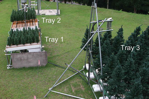
Tray 3 was a lysimeter consisting of wood plates and a plastic sheet placed on the ground, with a 360-cm square catchment area. The same number of large trees as in Trays 1 and 2 was used on Tray 3. Tree height on Tray 3 was extended to 240 cm with iron pipes 2.8 cm in outer diameter. Additional trees were placed along the outer edge of Tray 3 to avoid the edge effect. The arrangement of trees on trays is schematically shown in Murakami and Toba (2013). Each tray drained rainwater to a tipping-bucket flowmeter (see next section), and discharge from the tray was defined as net precipitation P_N that comprised both throughfall and stemflow.

Measurement began on 24 June 2012. Murakami and Toba (2013) began to measure on 24 May 2012; however, we used data beginning on 24 June because that was when measurement of single tree weight began. On 23 August, in the middle of the experiment, the number of trees on Trays 2 and 3 was reduced to 25; i.e. those stands were thinned. However, Tray 1 remained unthinned because it was the control. The experiment ended on 26 October 2012.

2.2 Instrumentation

P_G was measured using three raingauges. These were a storage-type gauge (homemade using copper alloy, 22.7 cm in diameter) and two tipping-bucket gauges, one 0.5 mm per tip (B-071-02-00, Yokokawa Denshi Co., Ltd., Tokyo) and the other 0.1 mm per tip (CTKF-0.1, Climatec Inc., Tokyo). Although the 0.1-mm gauge could measure the amount of rainfall, it was used to determine the temporal distribution of rainfall, e.g. the start and end of a rain event, because this gauge tended to underestimate rainfall amount relative to the 0.5-mm gauge. Rainfall measured by the 0.1-mm gauge was corrected using either the storage-type gauge or the 0.5-mm gauge, and analysed at a 5-min interval (Appendix A gives a detailed description of the method).

Three tipping-bucket type flowmeters, two 500 mL per tip (UIZ-TB500, Uizin Co., Ltd., Tokyo, for Tray 1; J-271-01-00, Yokogawa Co., Ltd., Tokyo, for Tray 2) and the other 2000 mL per tip (UIZ-TB2000, Uizin Co., Ltd., Tokyo, for Tray 3), were used at a measurement interval of 5 min. The resolution of P_N for Trays 1 and 2 was 0.333 mm, and that of Tray 3 was 0.154 mm. The weight of a single tree on Trays 1 and 3 was measured every minute using an electric balance (UX4200S, Shimadzu Corporation, Kyoto, Japan) and a digital push-pull gauge (RX-20, Aikoh Engineering Co., Ltd., Osaka, Japan), respectively, to monitor the influence of gusts on water storage. In actuality, the data fluctuated due to wind, and a 5-min average was used to calculate water balance. Tree weight on Tray 2 was assumed to be the same as that on Tray 1. Measurement resolution of tree weight was some 0.01 mm water equivalent on Trays 1 and 2, and around 0.1 mm on Tray 3, considering the influence of wind.

Net radiation R_n (Q*7, Radiation and Energy Balance Systems, Seattle, Washington, USA), air temperature T_a with RH (Sato Keiryoki Mfg. Co., Ltd., Tokyo, No. 7435–00 Hygro-station SK-5 RAD-SP), and wind speed u (Ikeda Keiki Co., Ltd., Tokyo, WM-30P) were measured above Tray 2. R_n, T_a with RH, and u were measured at 2.7 m, 2.5 m and 4.0 m above ground, respectively. The instrument used to measure T_a and RH was an aspirated psychrometer with a platinum resistance thermometer for the dry and wet bulb sensors. The accuracy of T_a and RH was ±0.1°C and ±1%, respectively. The interval of measurement for R_n, T_a, RH and u was 1 min, but 5-min average data were used for analysis.

2.3 Separation of rainfall into rain and sub-rain events

Rainfall is intermittent, and the end of a rain event was defined if rainfall stopped for a certain period of time or more. The time duration to separate rainfall into each independent rain event was defined as separation time Spt, which was set at 6 h. In other words, if it stopped raining for 6 h or longer rainfall was divided into two independent rain events. During a rain event there might be a time when rainfall ceases temporarily, which was defined as the storm break time(s) Sbt (s). The rain event was divided into two or more sub-rain events with Sbt. In the present study Sbt was set at 20 min. The start and end time of the i-th sub-rain event (i-th storm break) were defined as t_Rsi and t_Rei (t_Bsi and t_Bei), respectively. Spt and Sbt satisfy the relationship 20 min ≤ Sbt < 6 h ≤ Spt. There appear many acronyms, abbreviations and symbols hereafter, and they are defined in Appendix B, Table B1.

A shorter Sbt is better in terms of temporal resolution. However, a too-short Sbt causes large error, because it takes some time for rainwater in the tray to reach the flowmeter. Just after the end of a sub-rain event with high rainfall intensity, changes in drainage were too rapid and too large to measure correctly within such a short Sbt. A 20-min Sbt was found by trial and error to be optimal.

2.4 Water balance on rain event and sub-rain event bases

On a rain-event basis, P_G, P_N and I have a simple relationship:

(1) $I=P_G-P_N$(1)

When a rain event consists of n sub-rain events, i.e. n − 1 storm break time, with total amount of P_G, it is expressed as

(2) $\begin{array}{rl}& P_G=\sum _{i=1}^n{P}_{Gi}=\sum _{i=1}^n\underset{t_{Rsi}}{\overset{t_{Rei}}{\int }}Rdt=\sum _{i=1}^n\left[\underset{t_{Rsi}}{\overset{t_{Rei}}{\int }}Ddt+\underset{t_{Rsi}}{\overset{t_{Rei}}{\int }}Edt\right]+\\ & \sum _{i=1}^{n-1}\left[\underset{t_{Bsi}}{\overset{t_{Bei}}{\int }}Ddt+\underset{t_{Bsi}}{\overset{t_{Bei}}{\int }}Edt\right]+\mathrm{\Delta }S\end{array}$(2)

where P_Gi is P_G for the i-th sub-rain event, R is the rainfall rate, D is the drainage rate from the tray, and E is the evaporation rate. ΔS is the difference in water storage S between t_Ren and t_Rs1. It was assumed that S became zero at the end of Spt (= t_Ren + 6 h), which meant that the canopy dried out before the next rain event. Under the assumption that ΔS is zero in Equation (2)(2) $\begin{array}{rl}& P_G=\sum _{i=1}^n{P}_{Gi}=\sum _{i=1}^n\underset{t_{Rsi}}{\overset{t_{Rei}}{\int }}Rdt=\sum _{i=1}^n\left[\underset{t_{Rsi}}{\overset{t_{Rei}}{\int }}Ddt+\underset{t_{Rsi}}{\overset{t_{Rei}}{\int }}Edt\right]+\\ & \sum _{i=1}^{n-1}\left[\underset{t_{Bsi}}{\overset{t_{Bei}}{\int }}Ddt+\underset{t_{Bsi}}{\overset{t_{Bei}}{\int }}Edt\right]+\mathrm{\Delta }S\end{array}$(2) , S does not appear in Equation (1)(1) $I=P_G-P_N$(1) .

I during a sub-rain event I_R is given by

(3) $I_R=\sum _{i=1}^n{I}_{Ri}=\sum _{i=1}^n\underset{t_{Rsi}}{\overset{t_{Rei}}{\int }}Edt=\sum _{i=1}^n\left[\underset{t_{Rsi}}{\overset{t_{Rei}}{\int }}Rdt-\underset{t_{Rsi}}{\overset{t_{Rei}}{\int }}Ddt-\mathrm{\Delta }{S}_{Ri}\right]$(3)

where I_Ri is I_R for the i-th sub-rain event and ΔS_Ri is the difference in S between t_Rei and t_Rsi. Considering that R = 0 during Sbt, Equation (2)(2) $\begin{array}{rl}& P_G=\sum _{i=1}^n{P}_{Gi}=\sum _{i=1}^n\underset{t_{Rsi}}{\overset{t_{Rei}}{\int }}Rdt=\sum _{i=1}^n\left[\underset{t_{Rsi}}{\overset{t_{Rei}}{\int }}Ddt+\underset{t_{Rsi}}{\overset{t_{Rei}}{\int }}Edt\right]+\\ & \sum _{i=1}^{n-1}\left[\underset{t_{Bsi}}{\overset{t_{Bei}}{\int }}Ddt+\underset{t_{Bsi}}{\overset{t_{Bei}}{\int }}Edt\right]+\mathrm{\Delta }S\end{array}$(2) gives I during Sbt (I_Sbt).

(4) $I_{Sbt}=0forn=1$(4)

(5) $\begin{array}{rl}& I_{Sbt}=\sum _{i=1}^{n-1}{I}_{Sbti}=\sum _{i=1}^{n-1}\underset{t_{Bsi}}{\overset{t_{Bei}}{\int }}Edt=\sum _{i=1}^{n-1}\left[-\underset{t_{Bsi}}{\overset{t_{Bei}}{\int }}Ddt-\mathrm{\Delta }{S}_{Bi}\right]\\ & forn\ge 2\end{array}$(5)

where I_Sbti is I_Sbt for the i-th Sbt, and ΔS_Bi (≤0) is the difference in S between t_Bei and t_Bsi.

ΔS in Equation (2)(2) $\begin{array}{rl}& P_G=\sum _{i=1}^n{P}_{Gi}=\sum _{i=1}^n\underset{t_{Rsi}}{\overset{t_{Rei}}{\int }}Rdt=\sum _{i=1}^n\left[\underset{t_{Rsi}}{\overset{t_{Rei}}{\int }}Ddt+\underset{t_{Rsi}}{\overset{t_{Rei}}{\int }}Edt\right]+\\ & \sum _{i=1}^{n-1}\left[\underset{t_{Bsi}}{\overset{t_{Bei}}{\int }}Ddt+\underset{t_{Bsi}}{\overset{t_{Bei}}{\int }}Edt\right]+\mathrm{\Delta }S\end{array}$(2) is partitioned into drainage and evaporation after the cessation of rainfall. Hence, I after the cessation of rainfall is written as

(6) $I_{Aft}=\mathrm{\Delta }S-\underset{t_{Ren}}{\overset{t_{Ren+6}}{\int }}Ddt$(6)

On a rain event basis, I is calculated using P_G and P_N (Equation (1)(1) $I=P_G-P_N$(1) ), but Equations (3(3) $I_R=\sum _{i=1}^n{I}_{Ri}=\sum _{i=1}^n\underset{t_{Rsi}}{\overset{t_{Rei}}{\int }}Edt=\sum _{i=1}^n\left[\underset{t_{Rsi}}{\overset{t_{Rei}}{\int }}Rdt-\underset{t_{Rsi}}{\overset{t_{Rei}}{\int }}Ddt-\mathrm{\Delta }{S}_{Ri}\right]$(3) –6(6) $I_{Aft}=\mathrm{\Delta }S-\underset{t_{Ren}}{\overset{t_{Ren+6}}{\int }}Ddt$(6) ) can also yield canopy interception, which is defined as I’.

(7) $I{ }^{\mathrm{\prime }}=I_R+I_{Sbt}+I_{Aft}$(7)

Theoretically, Equations (1)(1) $I=P_G-P_N$(1) and (7(7) $I{ }^{\mathrm{\prime }}=I_R+I_{Sbt}+I_{Aft}$(7) ) yield the same result. However, they are not necessarily the same, because Equation (1)(1) $I=P_G-P_N$(1) is the difference between P_G and P_N, whereas Equation (7)(7) $I{ }^{\mathrm{\prime }}=I_R+I_{Sbt}+I_{Aft}$(7) is calculated using P_G, P_N and S. S includes some errors that are independent of P_G and P_N, which can make a difference between I and I’.

Murakami and Toba (2013) analysed rain events with P_G ≥ 0.1 mm. In the present study, rain events with P_G ≥ 0.5 mm were considered because P_N = 0 for P_G < 0.5 mm. If data were missing for one or more trays, data for the period were not analysed here, although Murakami and Toba (2013) used such data.

2.5 Wet canopy evaporation model using the PM equation for I_R and I_Sbt

A wet canopy evaporation model using the PM equation was applied that has the same structure as that of Saito et al. (2013), except for water storage calculation. In the present study, S was directly measured. Saito et al., in contrast, estimated S using water storage capacity and rainfall intensity. I was calculated for each sub-rain event and Sbt. I_Aft was not estimated using the model, but obtained using Equation (6)(6) $I_{Aft}=\mathrm{\Delta }S-\underset{t_{Ren}}{\overset{t_{Ren+6}}{\int }}Ddt$(6) .

(8) $I_{R\mathrm{\_}PM}=\sum _{i=1}^n{I}_{R\mathrm{\_}PMi}=\sum _{i=1}^n\left[\underset{t_{Rsi}}{\overset{t_{Rei}}{\int }}{E}_{Cal}dt\right]$(8)

(9) $I_{Sbt\mathrm{\_}PM}=0forn=1$(9)

(10) $I_{Sbt\mathrm{\_}PM}=\sum _{i=1}^{n-1}{I}_{Sbt\mathrm{\_}PMi}=\sum _{i=1}^{n-1}\left[\underset{t_{Bsi}}{\overset{t_{Bei}}{\int }}{E}_{Cal}dt\right]forn\ge 2$(10)

(11) $E_{Cal}=E_{PM}forS>E_{PM}\mathrm{\Delta }t$(11)

(12) $E_{Cal}=S/\mathrm{\Delta }tforS\le E_{PM}\mathrm{\Delta }t$(12)

The subscript “PM” represents calculation using the PM equation, and “i” indicates the i-th sub-rain event or Sbt. The calculation was done at 5-min intervals (Δt = 5 min), corresponding to the measurement interval of P_G and P_N. E_PM is the evaporation rate for a wet canopy surface, estimated by the PM equation:

(13) $E_{PM}=\frac{\mathrm{\Delta }}{\lambda \left(\mathrm{\Delta }+\gamma \right)}\left(R_n-G\right)+\frac{\rho C_P\left(q_S\left(T_a\right)-q\left(T_a\right)\right)}{\lambda \left(\mathrm{\Delta }+\gamma \right)r_a}$(13)

where Δ is the slope of the saturated specific humidity versus temperature curve; R_n is the net radiation; G is the ground heat flux (assumed to be zero); ρ is the air density; C_P is the specific heat of air; q_S(T_a) and q(T_a) are the saturated specific humidity and specific humidity at air temperature T_a, respectively; λ is the latent heat of vaporization; γ (=C_P/λ) is the psychrometric constant; and r_a is the aerodynamic resistance.

(14) $r_a=\frac{1}{k^{2}u}{\left\{ln\left(\frac{z-d}{z_0}\right)\right\}}^2$(14)

where k is the von Karman constant (0.4), z is the reference height (4.0 m above the ground, where the anemometer was placed), d is the zero plane distance, and z₀ is the roughness height length. d and z₀ were assumed to be 0.78 times and 0.08 times the tree height, respectively (Hattori 1985).

2.6 Estimation of SDE

Canopy interception during rainfall I_R comprises wet surface evaporation and SDE. I_R is derived from the water balance using Equation (3)(3) $I_R=\sum _{i=1}^n{I}_{Ri}=\sum _{i=1}^n\underset{t_{Rsi}}{\overset{t_{Rei}}{\int }}Edt=\sum _{i=1}^n\left[\underset{t_{Rsi}}{\overset{t_{Rei}}{\int }}Rdt-\underset{t_{Rsi}}{\overset{t_{Rei}}{\int }}Ddt-\mathrm{\Delta }{S}_{Ri}\right]$(3) , while wet surface evaporation during rainfall is calculated using Equation (8)(8) $I_{R\mathrm{\_}PM}=\sum _{i=1}^n{I}_{R\mathrm{\_}PMi}=\sum _{i=1}^n\left[\underset{t_{Rsi}}{\overset{t_{Rei}}{\int }}{E}_{Cal}dt\right]$(8) as I_{R_PM}. Therefore, SDE can be estimated as the difference between I_R and I_{R_PM}. Equation (15)(15) $I_{SDE}=I_R-I_{R\mathrm{\_}PM}$(15) calculates the component of canopy interception caused by SDE, I_SDE:

(15) $I_{SDE}=I_R-I_{R\mathrm{\_}PM}$(15)

3 Results

3.1 P_G and P_N for each tray

All P_G and P_N analysed are shown in Table 2 on a rain event basis. Monthly total rainfall and average air temperature at the site were, respectively, 191.5 mm and 24.6°C in July, 49.0 mm and 26.5°C in August, 215.5 mm and 23.0°C in September and 131.5 mm and 14.8°C in October. As mentioned in Section 2.4, some rain events were not analysed and are not included in Table 2.

Table 2. Gross rainfall (P_G) and net rainfall (P_N) for each tray on a rain event basis

Start of rain event		Duration	PG	PN	PN	PN	Rain event number
				Tray 1	Tray 2	Tray 3
		(h)	(mm)	(mm)	(mm)	(mm)
1 July 2012	16:00	10.3	4.5	3.3	3.0	2.6
2 July 2012	8:35	0.2	0.5	0.3	0.0	0.2
6 July 2012	13:45	52.2	110.2	101.3	101.6	98.5	Rain Event 1
12 July 2012	0:15	16.7	5.0	3.0	2.0	2.3
13 July 2012	2:45	0.3	0.5	0.3	0.3	0.0
14 July 2012	0:30	8.6	13.0	12.3	12.0	11.4
15 July 2012	5:05	3.9	0.5	0.0	0.0	0.0
20 July 2012	22:10	10.7	24.0	22.7	21.3	20.8
21 July 2012	20:25	0.6	0.5	0.0	0.0	0.0
22 July 2012	15:45	0.3	0.5	0.0	0.0	0.0
5 August 2012	23:50	0.9	0.5	0.0	0.0	0.0
12 August 2012	3:00	1.1	8.5	8.0	7.7	6.9
13 August 2012	13:25	0.3	3.5	2.3	0.3	2.0
13 August 2012	20:20	11.3	31.0	28.3	27.3	26.1	Rain Event 2
15 August 2012	19:10	7.0	0.5	0.0	0.0	0.0
17 August 2012	22:00	1.3	1.0	0.3	0.3	0.0
Total for before-thinning period			204.2	182.3	175.9	170.9
Thinned on 23 August
24 August 2012	17:35	2.0	0.5	0.0	0.3	0.2
27 August 2012	17:10	0.9	3.0	2.0	1.0	1.5
30 August 2012	7:30	0.8	0.6	0.3	0.3	0.3
30 August 2012	20:00	5.3	0.5	0.0	0.3	0.3
1 September 2012	16:25	1.8	5.5	4.3	3.7	3.9
4 September 2012	12:05	2.7	6.8	5.7	5.3	5.6
6 September 2012	8:20	3.5	27.0	24.7	22.0	23.7
11 September 2012	9:35	13.8	18.2	16.3	14.3	15.3
12 September 2012	16:40	0.7	5.3	4.7	4.3	4.8
15 September 2012	22:50	3.3	1.5	1.0	1.0	0.6
23 September 2012	4:05	13.7	14.8	13.0	12.3	13.0
24 September 2012	1:10	18.2	36.4	32.0	30.0	31.9	Rain Event 3
25 September 2012	9:05	0.1	0.5	0.0	0.0	0.0
30 September 2012	17:10	23.1	84.9	77.3	67.6	79.0	Rain Event 4
2 October 2012	0:55	5.7	2.0	1.7	1.7	1.7
2 October 2012	22:50	3.3	1.4	0.7	1.0	0.8
5 October 2012	2:55	0.4	2.0	1.7	1.7	1.4
6 October 2012	20:15	6.8	4.5	3.7	3.3	3.4
11 October 2012	17:35	10.4	10.8	9.3	8.7	9.1
13 October 2012	6:00	2.2	1.5	1.0	1.3	0.9
15 October 2012	11:05	0.8	2.0	1.3	1.3	1.4
17 October 2012	15:00	26.9	33.0	29.3	26.7	29.0
23 October 2012	7:30	26.3	28.0	24.3	19.7	24.1
25 October 2012	21:45	6.8	0.7	0.3	0.3	0.2
Total for after-thinning period			291.5	254.6	228.2	251.8

3.2 I, I_R, I_Sbt and I_Aft on a rain event basis

All panels in Fig. 2 show a clear linear relationship between P_G and I_R, with large determination coefficients r² ≥ 0.795. I_jR denotes I_R for Tray j (j = 1, 2, and 3), with the same convention for I_Sbt and I_Aft. Data shown in Fig. 2 are almost identical to those in Murakami and Toba (2013). However, the period of data used (see Section 2.1) and the size of the minimum rain event analysed (see Section 2.4) were slightly different.

Figure 2. Relationship between gross rainfall P_G and observed canopy interception during rainfall I_R, during storm break time I_Sbt and after cessation of rainfall I_Aft, on a rain event basis. (a) Tray 1 (control), (b) Tray 2 before thinning, (c) Tray 3 before thinning; (d) Tray 1 (control); (e) Tray 2 after thinning, (f) Tray 3 after thinning. In panel (c) for the largest P_G of 110.2 mm, the sum of I_3R and I_3Sbt is shown due to the clogged drain

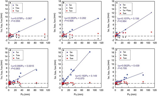
I_Sbt in each tray was nearly zero and tended to have negative values, which were caused by measurement error. This error was caused by the drainage term in Equation (5)(5) $\begin{array}{rl}& I_{Sbt}=\sum _{i=1}^{n-1}{I}_{Sbti}=\sum _{i=1}^{n-1}\underset{t_{Bsi}}{\overset{t_{Bei}}{\int }}Edt=\sum _{i=1}^{n-1}\left[-\underset{t_{Bsi}}{\overset{t_{Bei}}{\int }}Ddt-\mathrm{\Delta }{S}_{Bi}\right]\\ & forn\ge 2\end{array}$(5) due to time lag. The details are described in Appendix C.

For P_G ≥ about 5 mm, I_Aft reached a plateau around 1 mm, 1 mm and 2 mm before thinning for Trays 1, 2 and 3, respectively (Fig. 2(a–c)). After thinning, these values were around 1, 0.5 and 1 mm (Fig. 2(d–f)), corresponding to the reduction in tree density for Trays 2 and 3. However, Tray 1, the control, maintained the same value.

As shown in Table 3, the difference in I and I’ between trays was 7.5% or less, which was within the measurement error. I/P_G changed from 10.8% to 21.7% throughout the experiment, which is comparable with that in actual forests, although the experiments were conducted using plastic trees. I_R was the major constituent of I, i.e. I_R/I ranged from 67.3% to 93.8%, while I_Aft was minor. Considering the error of the flowmeters (see Section 2.2), I_Sbt was reasonably measured and was close to zero.

Table 3. Amount of rainfall and canopy interception before and after thinning for each tray

	PG	Number of rain events	Tray number	I	I’	I/I’	I/PG	IR	IR_PM	ISDE	ISbt	ISbt_PM	IAft	IR/I	ISDE/I
	(mm)			(mm)	(mm)	(%)	(%)	(mm)	(mm)	(mm)	(mm)	(mm)	(mm)	(%)	(%)
Before thinning	204.2	16	1	22.0	23.5	93.6	10.8	14.8	3.4	11.4	−0.8	17.0	9.5	67.3	52.0
			2	28.3	29.8	95.0	13.9	21.2	4.7	16.5	−1.5	21.7	10.1	74.9	58.3
			3*	33.4	36.1	92.5	16.3	24.3	4.9	19.4	−2.1	22.6	13.9	72.8	58.0
After thinning	291.5	24	1	37.0	36.3	101.9	12.7	26.1	16.5	9.6	−1.7	11.1	11.9	70.5	26.0
			2	63.3	63.2	100.2	21.7	59.4	20.9	38.5	−2.0	14.3	5.8	93.8	60.9
			3	39.7	38.1	104.2	13.6	28.7	22.4	6.3	−0.9	15.0	10.3	72.3	15.9

* In the rain event on 6 July (Rain Event 1) in Table 2 I_R and I_Sbt were not obtained independently due to clogging up of the drain, but the total value of I_R + I_Sbt was measured. In the event it was assumed that I_Sbt = 0, based on the results as shown in Fig. 2, and that I_R + I_Sbt = I_R.

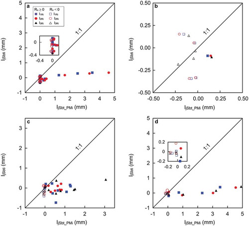
3.3 Comparison of I_R and I_{R_PM}, I_Sbt and I_{Sbt_PM} on a rain event basis with I_SDE

Observed values (I_R and I_Sbt) and calculated values (I_{R_PM} and I_{Sbt_PM}) are shown in Fig. 3. Before the thinning period, most I_{R_PM} values were nearly zero, although there were a few exceptions, i.e. some values of I_{R_PM} are around 2 mm (Fig. 3(a–c)). I_{Sbt_PM} fit to I_Sbt, i.e. close to zero, except for two rain events with P_G of 5.0 mm and 110.2 mm that had I_{Sbt_PM} between 8.1 mm and 11.3 mm. The rain event with P_G of 110.2 mm is referred to as “Rain Event 1” in the next section. The cause of the large I_{Sbt_PM} for those two rain events is unsuitable parameterization for the periods with larger positive R_n than the others, as discussed in Section 3.5. Each tray had a similar trend of reproducibility for I_{R_PM} and I_{Sbt_PM}, implying that not forest parameters but meteorological conditions mainly determined the calculated results.

Figure 3. Observed and calculated canopy interception during rainfall (respectively, I_R and I_{R_PM}) and during storm break time (respectively, I_Sbt and I_{Sbt_PM}), against gross rainfall P_G. (a) Tray 1 (control), (b) Tray 2 before thinning, (c) Tray 3 before thinning; (d) Tray 1 (control), (e) Tray 2 after thinning, (f) Tray 3 after thinning. Observed values and regression lines are the same as those in Fig. 2

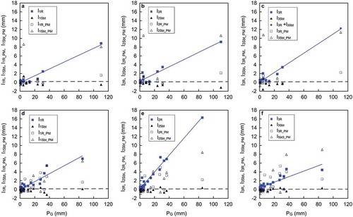
After the thinning period, estimated values of I_{R_PM} were greatly improved, even though many still underestimated I_R (Table 3, Fig. 3(d–f)). The reason why the reproducibility of I_{R_PM} was improved in the after-thinning period is described in Section 4.2. The reproducibility of I_{Sbt_PM} was much worse than in the before-thinning period, with large scatter. In the after-thinning period, each tray had the same trend of reproducibility. The cause of poorer estimation of I_{Sbt_PM}, i.e. overestimation, after thinning was also attributed to large R_n with inappropriate parameterization, discussed in Section 3.5.

In the before-thinning period, I_SDE for each tray was the predominant process of I, as I_SDE/I ranged from 52.0 to 58.3% (Table 3). In the after-thinning period, I_SDE/I showed smaller values, of 26.0% in Tray 1 and 15.9% in Tray 3 (the cause is discussed in Sections 4.2 and 4.6). I_SDE was a major process only in Tray 2, with I/I_SDE of 60.9% in the after-thinning period.

3.4 P_G, I_R, I_{R_PM} and I_SDE for four heavy rain events

As a general trend, the longer the rainfall duration, the greater the number of sub-rain events. Kondo et al. (1992) and Návar (2020) found that the rainfall duration tends to become longer with increasing rainfall amount, although the correlation between the two variables was not very high. As a consequence, the number of sub-rain events is expected to increase with the rainfall amount. A rain event with many sub-rain events tends to include larger variation in meteorological conditions than those with fewer sub-rain events. Analysing such a rain event is an effective approach to investigate the response of canopy interception to meteorological factors.

The two heaviest rain events in each of the before-thinning and after-thinning periods (Table 2) were selected, and we conducted a detailed analysis of P_G, I_R, I_{R_PM} and I_SDE. The before-thinning period had rain events with P_G of 110.2 mm (Rain Event 1 with 22 sub-rain events) and 31.0 mm (Rain Event 2 with six sub-rain events) as shown in Table 4. These two rain events accounted for 69.1% of total rainfall in the before-thinning period (Table 3). In the after-thinning period, we selected one with P_G of 36.4 mm (Rain Event 3 with 14 sub-rain events) and another with 84.9 mm (Rain Event 4 with eight sub-rain events). These two rain events accounted for 41.6% of total rainfall in the after-thinning period (Table 3).

Table 4. Amount of rainfall and canopy interception during four heavy rain events. Each value represents the total amount, although the sum operator is omitted

	Rain event	PG	Number of sub-rain events	Tray number	I	I’	I/I’	I/PG	IR	IR_PM	ISDE	ISbt	IAft	IR/I	ISDE/I
		(mm)			(mm)	(mm)	(%)	(%)	(mm)	(mm)	(mm)	(mm)	(mm)	(%)	(%)
Before thinning	1	110.2	22	1	8.9	9.5	94.4	8.1	8.8	1.6	7.2	−0.5	1.1	98.3	80.5
				2	8.6	9.5	90.9	7.8	9.2	2.2	7.0	−1.2	1.5	106.8	81.2
				3 *	11.7	14.5	81.0	9.6	−	2.3	−	−	2.2	−	−
	2	31.0	6	1	2.7	2.6	102.6	8.6	2.5	−0.2	2.7	−0.6	0.7	93.4	100.8
				2	3.7	3.6	101.9	11.9	3.5	−0.2	3.7	−0.6	0.7	95.2	100.6
				3	4.9	5.0	99.2	15.9	3.4	−0.2	3.6	−0.3	1.8	69.1	73.1
After thinning	3	36.4	14	1	4.4	4.1	108.1	12.2	5.4	2.9	2.5	−1.2	−0.1	121.7	56.4
				2	6.4	6.4	100.0	17.7	6.9	3.2	3.7	−0.2	−0.2	107.2	57.5
				3	4.5	4.5	100.5	12.4	4.6	4.0	0.6	−0.4	0.2	102.1	13.3
	4	84.9	8	1	7.6	7.6	100.0	9.0	7.0	1.7	5.3	0.1	0.5	91.9	69.5
				2	17.3	17.3	100.0	20.4	16.3	2.2	14.1	0.4	0.6	94.3	81.6
				3	6.0	5.8	103.6	7.0	4.4	2.4	2.0	0.3	1.0	73.7	33.5

* I_R and I_Sbt were not obtained due to clogging up of the drain, and I_SDE was not calculated.

In Table 4, values of I/I’ are 90.9% to 108.1%, which were within the range of measurement error, except for an outlier of 81.0% in Tray 3 for Rain Event 1 that might be related to the clogging up of the drain. Some values of I_R/I and I_SDE/I were over 100% due to measurement errors. I_R was a major component of I. I_SDE was also a predominant process of I, although in Tray 3 I_SDE/I values for Rain Events 3 and 4 were 13.3% and 33.5%, respectively, which were much smaller than the others (Table 4). It is estimated that wet surface evaporation was the major evaporation process in Tray 3 for Rain Events 3 and 4. During Rain Event 2, the values of I_SDE/I were larger than I_R/I in all trays, while for all the other events that was not the case. I_SDE was calculated as the residual between I_R and I_{R_PM}, as shown in Equation (15)(15) $I_{SDE}=I_R-I_{R\mathrm{\_}PM}$(15) . In all trays, I_{R_PM} values for Rain Event 2 were −0.2 (<0), which meant water vapour condensed on trees in the calculation. Negative values of I_{R_PM} seemingly boosted I_SDE whether actual SDE increased or not, which was the cause of I_SDE/I > I_R/I during Rain Event 2.

Figure 4(a–d), corresponding to Rain Events 1–4, respectively, indicates the relationship between P_Gi and I_jRi, where I_jRi is I_R for Tray j (i = 1, 2 and 3) for the i-th sub-rain event. Solid and open symbols represent I_jRi with R_n ≥ 0 and R_n < 0, respectively. Regression lines shown in Fig. 4(a–d) were calculated irrespective of the sign of R_n. Eleven regression lines were calculated, all of which showed r² ≥ 0.5 (range 0.574–0.999). In Tray 3 before thinning, the regression line for Rain Event 1 (Fig. 4(a)) was unavailable because of missing data. The largest I_3Ri in Fig. 4(b) for Tray 3 was 2.2 mm, but in Murakami and Toba (2013) the value was mistakenly presented as 4.1 mm.

Figure 4. (a–d) Gross rainfall for the i-th sub-rain event P_Gi and observed canopy interception during rainfall for the sub-rain event I_jRi in Tray j for four heavy rain events. (e–h) Calculated canopy interception during rainfall for the i-th sub-rain event I_{jR_PMi} and that of observed I_jRi for four heavy rain events in Tray j. (a) and (e) Rain Event 1 with total gross rainfall (P_G) of 110.2 mm before thinning period; (b) and (f) Rain Event 2 with P_G of 31.0 mm before thinning period; (c) and (g) Rain Event 3 with P_G of 36.4 mm after thinning period; (d) and (h) Rain Event 4 with P_G of 84.9 mm after thinning period

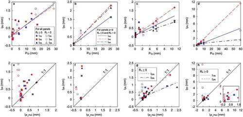
The inclination of the regression line for a certain tray was not necessarily constant in each period, i.e. within the before-thinning or the after-thinning period. At the same time, change in the inclination between rain events was different depending on the tray. For instance, in Tray 2 the inclination is almost the same between Rain Events 3 and 4 (red broken lines in Fig. 4(c,d)), while in Tray 3 it drastically declines (black long dashed dotted lines in Fig. 4(c,d)). Figure 4(e–h), corresponding respectively to Rain Events 1–4, shows the relationship between I_{jR_PMi} and I_jRi for each tray. Regression lines were calculated for I_jRi with R_n ≥ 0, and are shown if r² ≥ 0.5. Four out of nine regression lines indicated r² ≥ 0.5. All regression lines that were calculated combining I_jRi with both R_n ≥ 0 and R_n < 0 resulted in r² < 0.5. Regression lines derived from I_jRi with R_n < 0 gave r² < 0.5. The results in Fig. 4 imply that I_{jR_PMi} can estimate I_jRi only when R_n ≥ 0; however, the estimation using P_Gi on a sub-rain event basis (Fig. 4(a–d)) is much better than that of I_{jR_PMi} (Fig. 4(e–h)). All I_{jR_PMi} with R_n < 0 were negative, but only a small number of results for I_jRi with R_n < 0 were negative.

3.5 P_G, I_Sbt and I_{Sbt_PM} for four heavy rain events

Figure 5(a–d), corresponding respectively to Rain Events 1–4, shows measured and calculated I during Sbt on a storm break time basis in Tray j, i.e. I_jSbti and I_{jSbt_PMi}, respectively. Although measured I_Sbt on a rain event basis tended to show negative values, e.g. typically −1 mm, due to measurement errors (Fig. 2), those of I_Sbt on a storm break time basis were much smaller because they were divided into each storm break time. Specifically, I_jSbti with R_n < 0 ranged from −0.402 to 0.343 mm, which is comparable with the measurement resolution of P_N in Trays 1 and 2 (0.333 mm). All I_{jSbt_PMi} with R_n < 0 had negative values, with a minimum of −0.219 mm. Data for I_jSbti with R_n ≥ 0 were within −0.735 to 0.428 mm. Nevertheless, I_{jSbt_PMi} with R_n ≥ 0 seriously overestimated I_jSbti, except for Rain Event 2 (Fig. 5(b)), which had only one I_jSbti result with R_n ≥ 0. This overestimation was attributed to inappropriate parameterization.

Figure 5. Observed canopy interception during storm break time I_jSbti and calculated I_{jSbt_PMi} on a storm break time basis in Tray j. (a) Rain Event 1 before thinning period; (b) Rain Event 2 before thinning period; (c) Rain Event 3 after thinning period; (d) Rain Event 4 after thinning period

As stated in Section 3.2 and Table 3, I_Sbt was nearly zero on a rain event basis in both the before- and after-thinning periods. Unsuitable parameterization for the periods with R_n ≥ 0 was the cause of overestimation originating from capillary water in trees. The details are described in Appendix D.

3.6 Time course of I_R, I_{R_PM}, I_Sbt and I_{Sbt_PM}

A couple of time series for measured and/or calculated components, P_G, S, $\sum _{i=1}^n{I}_{jRi},$ $\sum _{i=1}^n{I}_{jR\mathrm{\_}PMi},$ $\sum _{i=1}^{n-1}{I}_{jSbti}$, $\sum _{i=1}^{n-1}{I}_{jSbt\mathrm{\_}PMi}$ (hereafter, the last four are denoted as ΣI_jRi, ΣI_{jR_PMi}, ΣI_jSbti and ΣI_{jSbt_PMi} for simplicity) potential evaporation E_PM calculated by the PM equation, and micrometeorological data R_n, RH, T_a and u are shown in Fig 6 and Fig 7, which correspond to Rain Events 1 and 4, respectively. “Night-time” in figures represents from sunset to sunrise. The time course of ΣI_jRi and ΣI_jSbti is shown in stepwise fashion because they were calculated on a sub-rain event basis and on an Sbt basis, respectively, based on water balance. That means it took some time for rainwater on the tray and in the tube to reach the flowmeter, and 5 min was too short in many cases. Note that I_jRi and I_jSbti are the difference between ΣI_jRi and ΣI_jRi-1 and ΣI_jSbti and ΣI_jSbti-1 for i ≥ 2, respectively, and ΣI_jR1 = I_jR1 and ΣI_jSbt1 = I_jSbt1 for i = 1. Other data, including ΣI_{jR_PMi} and ΣI_{jSbt_PMi}, are plotted every 5 min.

Figure 6. Time series of water budget, canopy interception and meteorological elements for Rain Event 1 with total gross rainfall P_G of 110.2 mm, before thinning: (a) P_G; (b) canopy storage S; (c) observed cumulative I_jRi; (d) calculated cumulative I_{jR_PMi}; (e) observed cumulative I_jSbti; (f) calculated cumulative I_{jSbt_PMi}; (g) calculated potential evaporation E_PM; (h) net radiation R_n; (i) relative humidity RH; (j) air temperature T_a; (k) wind speed u. Unit of ordinates is mm unless otherwise indicated

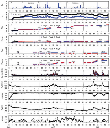
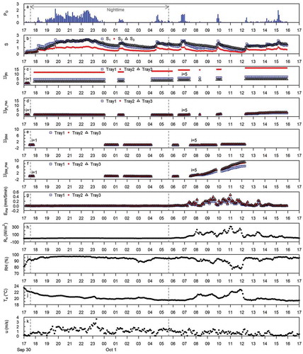
Figure 7. Time series of water budget, evaporation and meteorological elements for Rain Event 4 with total gross rainfall P_G of 84.9 mm, after thinning; details on each panel are the same as in Fig. 6

Rain Event 1 (Fig. 6) began at 13:45 on 6 July 2012 Japan Standard Time. Water storage in Trays 1 and 3 (S₁ and S₃, respectively) increased or decreased with rainfall. As mentioned in Section 2.2, S₂ in Tray 2 was assumed to be the same as in Tray 1. For Tray 3, ΣI_3Ri, ΣI_{3R_PMi}, ΣI_3Sbti and ΣI_{3Sbt_PMi} are shown through 17:15 on 6 July, because the drain of the tray clogged (see Fig. 2 caption). In Trays 1 and 2, ΣI_jRi increased with P_G throughout Rain Event 1, except for three sub-rain events (total decreases were 0.24 and 0.21 mm for Trays 1 and 2, respectively, but this is difficult to read from Fig. 6(c) because of small changes), which was caused by measurement errors. At the end of Rain Event 1, ΣI_1Ri and ΣI_2Ri, i.e. I_1R and I_2R, were 8.8 and 9.2 mm, respectively, but ΣI_{1R_PMi} and ΣI_{2R_PMi}, i.e. I_{1R_PM} and I_{2R_PM}, were only 1.6 and 2.2 mm, respectively (Fig. 6(c–d), Table 4). The underestimation of ΣI_{jR_PMi} was attributed to negative E_PM, reflecting R_n < 0 during night-time (Fig. 6(g)). During night-time on 7–8 July, ΣI_{jR_PMi} decreased (again, this is difficult to read in Fig. 6(d)), which meant condensation, not evaporation, occurred. Condensation also occurred during night-time on 30 September–1 October (Fig. 7(d)).

The greatest discrepancy between I_R and I_{R_PM} during night-time is shown in Fig. 4(h) and Fig. 7 (for i = 2, 17:55 on 30 September through 0:00 on 1 October). For the sub-rain event with P_G2 = 59.6 mm, I_1R2, I_2R2 and I_3R2 were 4.2, 11.6 and 1.7 mm (open square on the middle left, circle on the upper left and triangle on the lower left in Fig. 4(h), which corresponds to Fig. 7(c) for i = 2), respectively, while changes in I_{1R_PM}, I_{2R_PM} and I_{3R_PM} between i = 2 and i = 1 were −0.1, −0.2 and −0.2 mm, respectively (in Fig. 7(d)).The PM equation did not function at all as a predictive method.

Obviously, I_jRi was controlled by P_Gi instead of I_{jR_PMi} (that is, E_PM), as seen in Fig. 4(a–d). Meteorological factors RH, T_a and u (except for R_n during daytime) do not necessarily correlate with E_PM but with R_n (Fig 6 and Fig 7). I_{jR_PMi} was valid only when R_n ≥ 0, but R_n was independent of P_Gi. P_Gi controlled I_jRi and ΣI_jRi, regardless of the sign of R_n.

ΣI_jSbti values in Fig 6(e) and Fig 7(e) are nearly equal to zero, corresponding to those in Fig. 5(a,d), respectively. However, in Fig 6(f) and Fig 7(f) ΣI_{jSbt_PMi} values rise in daytime when E_PM shows high values due to large R_n, which caused overestimation in combination with capillary water in the trees, as mentioned in the previous section.

4 Discussion

4.1 Increase in I after thinning

Some studies showed that I declined after thinning (Teklehaimanot et al. 1991, Shinohara et al. 2015, Sun et al. 2015) or diminished with decreasing stand density (Komatsu et al. 2008), but no study has demonstrated a rise in I after thinning. Unexpectedly, I in Tray 2 increased after thinning (Table 3, Figs 2(b,e), 3(b,e)). The increase in I was observed on a rain event basis and was proportional to the rainfall amount for each rain event. That held true on a sub-rain event basis, as shown in Fig. 4(a−d). The largest rain event after thinning was Rain Event 4, the time course for which is shown in Fig. 7. The water storage on Tray 2 (red circles in Fig. 7(b)) was the smallest among the three trays. That meant Tray 2 was the least evaporative with the smallest wet surface area. The values of r_a for Tray 2 before and after thinning were assumed to be identical, because the two stands had the same tree heights (Equation (14)(14) $r_a=\frac{1}{k^{2}u}{\left\{ln\left(\frac{z-d}{z_0}\right)\right\}}^2$(14) ). Considering the smallest water storage and the values of r_a for Tray 2, I_{R_PM} and I_{Sbt_PM} after thinning must decrease in terms of wet canopy evaporation. After all, there is no prospect that the increase in I can be elucidated by the PM equation, i.e. wet surface evaporation. It is presumed that thinning in Tray 2 promoted the production of splash droplets and/or ventilation, although this must be confirmed by additional measurements, analyses and studies.

4.2 Validity and limitations of the PM equation

During night-time, almost all I_{jR_PMi} values for Rain Events 1–4 were negative, reflecting R_n < 0, meaning that water vapour condensed on the canopy surface instead of evaporating (Fig. 4(e–h)). In contrast, measurements showed that I_jRi with R_n < 0 had positive values (Figs 4(e−h), 6 and 7) except for some sub-rain events depicted in Fig. 6, an exception caused by measurement error (see Section 3.6). The discrepancy between I_{jR_PMi} and I_jRi was very large, and it is obvious that the PM equation did not work at night when R_n < 0 (Section 3.6).

The aerodynamic term (the second term on the right side of Equation (13)(13) $E_{PM}=\frac{\mathrm{\Delta }}{\lambda \left(\mathrm{\Delta }+\gamma \right)}\left(R_n-G\right)+\frac{\rho C_P\left(q_S\left(T_a\right)-q\left(T_a\right)\right)}{\lambda \left(\mathrm{\Delta }+\gamma \right)r_a}$(13) ) was small during the sub-rain event because of high RH, especially when the wind was weak. In that case, the radiation term (the first term on the right side of Equation (13)(13) $E_{PM}=\frac{\mathrm{\Delta }}{\lambda \left(\mathrm{\Delta }+\gamma \right)}\left(R_n-G\right)+\frac{\rho C_P\left(q_S\left(T_a\right)-q\left(T_a\right)\right)}{\lambda \left(\mathrm{\Delta }+\gamma \right)r_a}$(13) ) controlled E_PM. At night, R_n was negative and, as a consequence, E_PM during the sub-rain event became negative during night-time (Fig 6 and Fig 7). In daytime, the aerodynamic term remained small during the sub-rain event, but more often than not, R_n became positive, resulting in E_PM ≥ 0. This observation indicates that I_jSbti was nearly zero and that I_jRi accounted for the major part of I, irrespective of the sign of R_n, i.e. regardless of daytime or night-time (Tables 3 and Tables 4, Fig 6 and Fig 7). I_{jR_PMi} with R_n ≥ 0 could reproduce I_jRi (Fig. 4(e–h)), but estimation using P_G was better than the model (Fig. 4(a–d)). The reproducibility of I_{R_PM} improved in the after-thinning period (see Section 3.3 and Fig. 3), because there were more rain events with R_n ≥ 0 during rainfall after thinning than before thinning.

Tsukamoto et al. (1988) conducted a water balance experiment using a single Japanese cedar tree placed in a stand. They measured P_G, P_N and tree weight under natural rainfall on an hourly basis, showing that I_R was proportional to P_G for a sub-rain event, with I_Sbt nearly zero. They also indicated that I_Sbt and/or I_Aft were close to zero if solar radiation was nil, but that the values increased with increasing radiation. Although we used artificial Christmas trees, the results were the same as those of Tsukamoto et al. (1988). Our study and that of Tsukamoto et al. are consistent with the observational fact that I_R is independent of the radiative energy received by the canopy. Similarly, Pearce et al. (1980) found that hourly evaporation rates during daytime and night-time were the same. Thus, we conclude that the PM-based model contradicts the measurements, although it can work when R_n > 0.

I_SDE is calculated using Equation (15)(15) $I_{SDE}=I_R-I_{R\mathrm{\_}PM}$(15) as the difference between I_R and I_{R_PM}, which means I_SDE declines with increasing positive R_n, as I_{R_PM} is boosted by R_n. However, whether SDE actually decreases with R_n or not remains a problem to be solved, because in the present study I_SDE was not measured directly but rather was taken as the residual between measured I_R and calculated I_{R_PM}.

4.3 Do splash droplets drift or evaporate?

Some studies assert that small droplets are transported somewhere by turbulence instead of being eliminated by evaporation (Hashino et al. 2010, Saito et al. 2013). The foundation of such studies was that terminal velocities of droplets with diameters 10, 20 and 50 µm are, respectively, 0.3, 1.2 and 7.6 cm s^-1. This means that the droplets are easily transported by weak wind and do not fall on the ground, because they are aerosols. Nonetheless, airborne droplets are captured by canopy again and observed as fog precipitation. This results in a contradiction, because the precipitation increases P_N and reduces I. For example, in tropical montane cloud forests fog precipitation accounts for between 2% and 45% of incident annual rainfall (Bruijnzeel et al. 2011). In Japan it is reported that cloud water deposition was more than 100% of annual rainfall (Kobayashi et al. 2001, Igawa et al. 2002). Apart from the transport of small droplets, first and foremost, it is impossible for such droplets to survive in the air without evaporation, even under high RH. They can survive stably only when the air is in saturation or supersaturation with respect to liquid water. Although E_PM is a function of some meteorological variables, evaporation of a small droplet is a function of T_a and RH in addition to the initial diameter (Holterman 2003). That means SDE must be calculated independent of the PM equation. The big difference between wet surface evaporation and SDE is that the surface evaporation rate saturates if the surface is completely wet, but the SDE rate increases with an increasing number of droplets and a decreasing diameter of the droplets. This implies that a slight change in the splash droplet size distribution, which is dictated by the raindrop size distribution and tree structures, can make a significant difference in the amount of SDE.

The lifetime of a small droplet under RH of 95% and 99% is shown in Fig. 8. It is strongly dependent on RH and the initial diameter. Figure 8 was calculated based on Holterman (2003), which was developed to evaluate spray drift of agricultural chemicals. Another approach to calculate the evaporation of a small droplet is the theory of cloud physics. Murakami (2006) estimated the lifetime of a small droplet using the cloud physical approach (Beard and Pruppacher 1971) that included much more complicated mathematical processes. For a droplet of 50 μm in diameter with RH of 95% the estimated lifetimes in Fig. 8 and Murakami (2006) were, respectively, 58 s and 73 s at 10°C, 48 s and 61 s at 15°C, and 13 s and 47 s at 25°C. Unfortunately, the discrepancy between the two methods was 362% at 25°C. Assuming RH of 96% instead of 95%, lifetimes in Fig. 8 became longer and almost the same as those of Murakami (2006): 72 s at 10°C, 60 s at 15°C and 45 s at 25°C. Considering the measurement accuracy of RH, i.e. ±1% at best, both estimations are within the measurement error range.

Figure 8. Dependence of lifetime for small droplets on relative humidity (RH) and air temperature. (a) RH = 95%; (b) RH = 99%

As shown in Fig. 8 and Murakami (2006), splash droplets do not drift and survive in the air but evaporate and disappear during rainfall. If the splash droplet size distribution and the production rate are measured, it is possible to calculate SDE. Splash droplet size distribution can be measured using an aerosol spectrometer. It is challenging but required for the development of forest hydrology.

4.4 Heat source of latent heat of vaporization

Stewart (1977) showed that in a pine forest when the canopy was wet, the flux of the latent heat of vaporization exceeded net radiation, and presumed that sensible heat originated upwind and was advected to the forest. Pearce et al. (1980) also concluded that not net radiation but advected energy drives evaporation of a wet canopy. However, it seems unlikely that the latent heat continues to advect during a long-lasting rainfall event, and if the advection had been the energy source, the PM equation that takes in situ meteorological factors into consideration could have successfully predicted I. There must be an alternative mechanism and source.

Latent heat of vaporization for I_2R2 in Fig. 7 (for i = 2, 17:55 on 30 September to 0:00 on 1 October) was 1294 W m^-2, as large as the solar constant (1370 W m^-2). Jiménez-Rodríguez et al. (2021) pointed out that during rainfall the temperature difference between the forest floor and the air in the forest creates an atmosphere unstable that causes vertical mixing. This mechanism transports water vapour upward. However, it is difficult for soil to exchange heat with the atmosphere due to nearly zero wind speed at the ground surface. Clouds, where condensation occurs constantly, are the only possible heat source. There are four possible mechanisms for transport of energy from the base of the cloud to the canopy, and at the same time it works as a mechanism to remove water vapour above the canopy.

First, the original air mass at the ground surface is squeezed upward by falling raindrops and the ambient air is dragged downward by those drops (Dunin et al. 1988). Second, an updraft driven by the difference in molar weight between water and dry air transports the vapour together with energy, called the “evaporative force” (Makarieva and Gorshkov 2007). The decrease in air volume caused by the removal of water vapour near the ground is essentially compensated for by the downdraft. Third, an updraft is caused by a reduction of air volume in the cloud due to water vapour condensation (Makarieva et al. 2013). Like the second process, the downdraft occurs automatically to compensate for the updraft. Fourth, the evaporation of water itself increases the air pressure around the canopy and causes an updraft because it involves an abrupt expansion: a phase change from liquid to gas. That is the opposite process of the third one and is proposed in the present study for the first time.

These four processes have not received much attention and have not been widely accepted. None has been proved by measurements and they are still hypotheses; however, those processes can elucidate the enigmatic problems: the mechanism of removal of water vapour from the canopy during rainfall, the heat source (i.e. latent heat released in the cloud upon condensation of water vapour), and the supply of sensible heat from the cloud (Murakami 2006). Vertical mixing of air between the ground surface and the cloud base provides a simple answer for the heat source enigma. Because water vapour and energy are always balanced by rapid vertical mixing, variations in T_a and RH caused by the exchange between the cloud and the ground surface are, seemingly, not observed.

4.5 Rainfall intensity, types of rainfall and traits of vegetation

As mentioned in the introduction, simulation using the PM equation revealed that I was not sensitive to rainfall intensity (Hall 2003). However, many studies including the present one showed that I increases with increasing rainfall amount or intensity, because actual evaporation process includes both wet surface evaporation and SDE, while Hall (2003) considered only wet surface evaporation.

Change in the inclination of the regression lines between rain events was different depending on the tray (Fig. 4(a−d), Section 3.4). That would be caused by the difference in rainfall intensity. In the after-thinning period, I_SDE/I was 26.0% in Tray 1 and 15.9% in Tray 3 (Table 3), but in the same period on a rain event basis it was 56.4% (Rain Event 3) and 69.5% (Rain event 4) in Tray 1 and 33.5% (Ran Event 4) in Tray 3 (Table 4). The difference in I_SDE/I on a period basis in Table 3 and on a rain event basis in Table 4 was more than double what would be caused by the change in rainfall intensity. A larger I_SDE/I would be the result of higher rainfall intensity that can produce more splash droplets. In fact, I_SDE/I in Rain Event 4 (the rainfall intensity derived from Table 2 was 3.7 mm h^-1) was greater than that in Rain Event 3 (2.0 mm h^-1) in all trays (Table 4).

The influence of rainfall intensity on rainwater partitioning including I is dependent on vegetation type. Janeau et al. (2015) showed that throughfall changes not only with rainfall intensity but also with vegetation type. In low-intensity rainfall vegetation with flexible leaves had high interception ability and yielded much stemflow, but in high-intensity rainfall it showed less interception ability due to the flexibility of leaves causing rainwater to fall down. In contrast, vegetation with rigid leaves had high interception ability at both low and high rainfall intensities because of their resistance against raindrop impact. In some vegetation types, leaf shape is more important than leaf amount. Liu and Zhao (2020) pointed out that Artemisia sacrorum Ledeb (less leaf amount, canopy cover and leaf area, but a fragmented leaf) showed less throughfall in comparison with Spiraea pubescens Turcz (larger leaf amount, canopy cover and leaf area, but a compact leaf), probably due to effective production of splash droplets.

Considering the above-mentioned facts, the amount of I is dependent on both the characteristics of trees and the type of rainfall (e.g. drizzle, widespread rain and thunderstorm), because the type of rainfall is relevant to the raindrop size distribution (Seela et al. 2018). However, there are few studies focusing on the relationship between traits of trees, types of rainfall and I. To deal with this issue, SDE is a key process that should be taken into account as SDE is dictated by those factors.

5 Conclusions

When net radiation (R_n) was positive, the PM equation could predict measured canopy interception during rainfall (I_R), although the accuracy was not high enough. However, the equation could not do so during night-time or when R_n was zero or negative. In many cases I_R was much larger than the predicted canopy interception using the PM equation (I_{R_PM}), which proved wet canopy evaporation is a minor process and SDE dictates canopy interception. Specifically, the ratio of SDE to total canopy interception, I_SDE/I, accounted for 52.0–58.3% and 15.9–60.9% in the before-thinning and the after-thinning periods, respectively, and on a rain event basis for 9 out of 11 rain events, I_SDE/I was over 56.4%.

The best predictor of I_R (and I also) was gross rainfall (P_G). I_R and P_G had a proportional relationship that implied rainfall itself is the driver of I_R. SDE could elucidate the proportional relationship between I_R and P_G, which is further evidence of the SDE hypothesis. Calculations indicated that splash droplets do not drift and survive during rainfall but evaporate and disappear in a short time even under high relative humidity, e.g. 99%.

Considering the latent heat of vaporization required, clouds are the only possible heat source. Vertical mixing of air between the ground surface and the cloud base caused by the difference in molar weight of gases, falling raindrops, condensation in the clouds and evaporation of canopy interception can be the driving force. However, there is little theoretical and observational knowledge of the transport mechanism during rainfall, so this knowledge should be pursued.

I depends not only on P_G or rainfall intensity but also on rainfall type and tree characteristics, although the relationship between I and type of rainfall and/or tree properties is little known. These unknown parts of canopy interception processes are strongly associated with SDE.

Acknowledgements

I am grateful to two anonymous reviewers for their useful and instructive comments.

Disclosure statement

No potential conflict of interest was reported by the author.

Additional information

Funding

This study was financially supported by JSPS KAKENHI [grant number 23580216].

Appendix A

Modification of rainfall amount measured by the 0.1-mm raingauge

The 0.1-mm raingauge underestimated rainfall amount in comparison with the storage-type gauge and the 0.5-mm gauge, but the degree of underestimation varied depending on the rain event. For example, for one rain event that started on 6 July the rainfall amount measured by the storage-type, the 0.5-mm and the 0.1-mm gauge was 110.2 mm, 110.5 mm and 104.3 mm (94.6% of the storage-type gauge), respectively, while for another rain event, on 6 September, the amount of rainfall measured by the storage-type, the 0.5-mm and the 0.1-mm gauge was 27.0 mm, 27.0 mm and 24.4 mm (90.4% of the storage-type gauge), respectively (see Table 2). Thus, either the storage-type or the 0.5-mm gauge was used to measure the rainfall amount. Rainfall with the storage gauge was measured manually at least every few days on weekdays but omitted on days off. Rainfall amount measured by the 0.1-mm gauge was modified based on that of the storage-type gauge on a rain event basis, but was corrected based on data measured by the 0.5-mm gauge when storage gauge data were missing. P_G was analysed at a 5-min interval.

Appendix B

Table B1. List of acronyms, abbreviations and symbols

Symbol	Unit	Description
γ	K^−1	Psychrometric constant
Δ	K^−1	Slope of the saturated specific humidity versus temperature curve
ΔS	mm	Difference in water storage between tRen and tRe1
ΔSBi	mm	Difference in water storage between tBei and tBsi
ΔSRi	mm	Difference in water storage between tRei and tRsi
Δt	h	Time interval (5 min)
λ	J kg^−1	Latent heat of vaporization
ρ	kg m^−3	Air density
CP	J kg^−1 K^−1	Specific heat of air
D	mm h^−1	Drainage rate from the tray
d	m	Zero plane distance
E	mm h^−1	Evaporation rate during rain event
Ecal	mm h^−1	Calculated evaporation rate
EPM	mm h^−1	Calculated evaporation rate using the Penman-Monteith equation
G	W m^−2	Ground heat flux
I	mm	Canopy interception
i	–	Ordinal number for the sub-rain event or the storm break time: i = 1, 2, …, n
I’	mm	Canopy interception calculated as the sum of IR, ISbt and IAft
IAft	mm	Canopy interception after cessation of rainfall
IjAft	mm	Canopy interception after cessation of rainfall for Tray j
IjR	mm	Canopy interception during rainfall for Tray j
IjRi	mm	Canopy interception during rainfall for Tray j for the i-th sub-rain event
IjR_PMi	mm	Canopy interception during rainfall for Tray j for the i-th sub-rain event calculated using the Penman-Monteith equation
IjSbt	mm	Canopy interception during storm break time for Tray j
IjSbti	mm	Canopy interception during storm break time for Tray j for the i-th storm break time
IjSbt_PMi	mm	Canopy interception during storm break time for Tray j for the i-th storm break time calculated using the Penman-Monteith equation
IR	mm	Canopy interception during rainfall
IRi	mm	Canopy interception during rainfall for the i-th sub-rain event
IR_PM	mm	Canopy interception during rainfall calculated using the Penman-Monteith equation
IR_PMi	mm	Canopy interception during rainfall for the i-th sub-rain event calculated using the Penman-Monteith equation
ISbt	mm	Canopy interception during storm break time
ISbti	mm	Canopy interception during storm break time for the i-th sub-rain event
ISbt_PM	mm	Canopy interception during storm break time calculated using the Penman-Monteith equation
ISbt_PMi	mm	Canopy interception during storm break time for the i-th storm break time calculated using the Penman-Monteith equation
ISDE	mm	Canopy interception during rainfall caused by splash droplet evaporation
j	–	Ordinal number for the tray: j = 1, 2 and 3
k	–	von Karman constant
n	–	Number of sub-rain events
PG	mm	Gross rainfall
PGi	mm	Gross rainfall for the i-th sub-rain event
PM	–	Penman-Monteith (equation)
PN	mm	Net rainfall
PVC	–	Polyvinyl chloride
q	kg kg^−1	Specific humidity
qs	kg kg^−1	Saturated specific humidity
R	mm h^−1	Rainfall rate
r^2	–	Determination coefficient
ra	s m^−1	Aerodynamic resistance
RH	%	Relative humidity
Rn	W m^−2	Net radiation
S	mm	Water storage
Sj	mm	Water storage for Tray j
Sbt	h	Storm break time
SDE	–	Splash droplet evaporation
Spt	h	Separation time to divide rainfall into two independent rain events
Ta	°C	Air temperature
tBei	h	Time of the end of the i-th storm break
tBsi	h	Time of the start of the i-th storm break
tRei	h	Time of the end of the i-th sub-rain event
tRsi	h	Time of the start of the i-th sub-rain event
u	m s^−1	Wind speed
z	m	Reference height
z0	m	Roughness height length

Appendix C

Cause of negative values of I_Sbt in Fig. 2

Ideally, rainwater stored on the stand S at the end of a sub-rain event would have been the only drainage source during the subsequent Sbt. However, in actuality, at the end of the sub-rain event, rainwater that would have drained during that sub-rain event from the trees prior to the Sbt of interest remained on the tray and in the tube leading to the flowmeters. The remaining rainwater was supplied as runoff D in Equation (5)(5) $\begin{array}{rl}& I_{Sbt}=\sum _{i=1}^{n-1}{I}_{Sbti}=\sum _{i=1}^{n-1}\underset{t_{Bsi}}{\overset{t_{Bei}}{\int }}Edt=\sum _{i=1}^{n-1}\left[-\underset{t_{Bsi}}{\overset{t_{Bei}}{\int }}Ddt-\mathrm{\Delta }{S}_{Bi}\right]\\ & forn\ge 2\end{array}$(5) , resulting in negative I_Sbt. The storage term in Equation (5)(5) $\begin{array}{rl}& I_{Sbt}=\sum _{i=1}^{n-1}{I}_{Sbti}=\sum _{i=1}^{n-1}\underset{t_{Bsi}}{\overset{t_{Bei}}{\int }}Edt=\sum _{i=1}^{n-1}\left[-\underset{t_{Bsi}}{\overset{t_{Bei}}{\int }}Ddt-\mathrm{\Delta }{S}_{Bi}\right]\\ & forn\ge 2\end{array}$(5) , ∆S_Bi, is always negative or zero, i.e. −∆S_Bi ≥ 0. Normally, the error caused by ∆S_Bi is smaller than that of the drainage term, because S measured by weighing devices has no delay time like drainage from trays, as well as a resolution higher than that of the drainage measurement (see Section 2.2).

Appendix D

Cause of overestimation of I_{Sbt_PM.}

According to Equations (8(8) $I_{R\mathrm{\_}PM}=\sum _{i=1}^n{I}_{R\mathrm{\_}PMi}=\sum _{i=1}^n\left[\underset{t_{Rsi}}{\overset{t_{Rei}}{\int }}{E}_{Cal}dt\right]$(8) –12(12) $E_{Cal}=S/\mathrm{\Delta }tforS\le E_{PM}\mathrm{\Delta }t$(12) ), evaporation rate E_Cal = E_PM for S > E_{_PM}∙∆t; otherwise, E_cal = S/∆t. Assuming that E_PM is sufficiently large for a wet canopy surface to dry out during Sbt and S = 0 is reached, E_Cal = S/∆t = 0 at the end of Sbt. However, the trees did not always dry out (S ≠ 0), even when E_PM maintained a large value over a long period. This was because under certain conditions, rainwater was not on the surface of the canopy but existed as capillary water. The trees were made of PVC imitation leaves that were inserted in twisted iron lines. Rainwater was stored in the spaces of the twisted iron lines and PVC leaves as capillary water, which was difficult to evaporate. In other words, the actual r_a was much larger than that calculated by Equation (14)(14) $r_a=\frac{1}{k^{2}u}{\left\{ln\left(\frac{z-d}{z_0}\right)\right\}}^2$(14) . Because the objective of the present study was not to reproduce I_Sbt but to evaluate the amount of SDE and the validity and limitations of the PM equation, optimization of r_a for I_{jSbt_PMi} with R_n ≥ 0 was not carried out.

References

- Allen, S.T., et al., 2017. The role of stable isotopes in understanding rainfall interception processes: a review. WIREs Water, 4, e1187. doi:10.1002/wat2.1187
- Beard, K.V. and Pruppacher, H.R., 1971. A wind tunnel investigation of the rate of evaporation of small water drops falling at terminal velocity in air. Journal of Atmospheric Sciences, 28 (8), 1455–1464. doi:10.1175/1520-0469(1971)028<1455:AWTIOT>2.0.CO;2
- Bruijnzeel, L.A., Mulligan, M., and Scatena, F.N., 2011. Hydrometeorology of tropical montane cloud forests: emerging patterns. Hydrological Processes, 25 (3), 465–498. doi:10.1002/hyp.7974
- Carlyle-Moses, D.E. and Price, A.G., 1999. An evaluation of the Gash interception model in a northern hardwood stand. Journal of Hydrology, 214 (1–4), 103–110. doi:10.1016/S0022-1694(98)00274-1
- Deguchi, A., Hattori, S., and Park, H., 2006. The influence of seasonal changes in canopy structure on interception loss: application of the revised Gash model. Journal of Hydrology, 319 (1–4), 80–102. doi:10.1016/j.jhydrol.2005.06.005
- Dunin, F.X., O’Loughlin, E.M., and Reyenga, W., 1988. Interception loss from eucalypt forest: lysimeter determination of hourly rates for long term evaluation. Hydrological Processes, 2 (4), 315–329. doi:10.1002/hyp.3360020403
- Dunkerley, D.L., 2009. Evaporation of impact water droplets in interception processes: historical precedence of the hypothesis and a brief literature overview. Journal of Hydrology, 376 (3–4), 599–604. doi:10.1016/j.jhydrol.2009.08.004
- Fan, Y., et al., 2019. Reconciling canopy interception parameterization and rainfall forcing frequency in the community land model for simulating evapotranspiration of rainforests and oil palm plantations in Indonesia. Journal of Advances in Modeling Earth Systems, 11 (3), 732–751. doi:10.1029/2018MS001490
- Gash, J.H.C., 1979. An analytical model of rainfall interception by forests. Quarterly Journal of the Royal Meteorological Society, 105 (443), 43–55. doi:10.1002/qj.49710544304
- Gash, J.H.C., Lloyd, C.R., and Lachaud, G., 1995. Estimating sparse forest rainfall interception with an analytical model. Journal of Hydrology, 170 (1–4), 79–86. doi:10.1016/0022-1694(95)02697-N
- Ghimire, C.P., et al., 2012. Rainfall interception by natural and planted forests in the Middle Mountains of Central Nepal. Journal of Hydrology, 475, 270–280. doi:10.1016/j.jhydrol.2012.09.051
- Ghimire, C.P., et al., 2017. Measurement and modeling of rainfall interception by two differently aged secondary forests in upland eastern Madagascar. Journal of Hydrology, 545, 212–225. doi:10.1016/j.jhydrol.2016.10.032
- Hall, R.L., 2003. Interception loss as a function of rainfall and forest types: stochastic modelling for tropical canopies revisited. Journal of Hydrology, 280 (1–4), 1–12. doi:10.1016/S0022-1694(03)00076-3
- Hashino, M., Yao, H., and Tamura, T., 2010. Micro-droplet flux in forest and its contribution to interception loss of rainfall – theoretical study and field experiment. Journal of Water Resource and Protection, 2 (10), 872–879. doi:10.4236/jwarp.2010.210104
- Hattori, S., 1985. Explanation on derivation process of equations to estimate evapotranspiration and problems on the application to forest stand. Bulletin of the Forestry and Forest Products Research Institute, 332, 139–165. in Japanese.
- Holterman, H.J., 2003. Kinetics and evaporation of water drops in air. Wageningen, The Netherlands, IMAG Report No. 2003-12.
- Hörmann, G., et al., 1996. Calculation and simulation of wind controlled canopy interception of a beechforest in northern Germany. Agricultural and Forest Meteorology, 79 (3), 131–148. doi:10.1016/0168-1923(95)02275-9
- Igawa, M., Tsutsumi, Y., and Okochi, H., 2002. High frequency and large deposition of acid fog on high elevation. Environmental Science and Technology, 32 (1), 1–6. doi:10.1021/es0105358
- Janeau, J.L., Grellier, S., and Podwojewski, P., 2015. Influence of rainfall interception by endemic plants versus short cycle crops on water infiltration in high altitude ecosystems of Ecuador. Hydrology Research, 46 (6), 1008–1018. doi:10.2166/nh.2015.203
- Jeong, S., Otsuki, K., and Farahnak, M., 2019. Relationship between stand structures and rainfall partitioning in dense unmanaged Japanese cypress plantations. Journal of Agricultural Meteorology, 75 (2), 92–102. doi:10.2480/agrmet.D-18-00030
- Jiménez-Rodríguez, C.D., et al., 2021. Vapor plumes in a tropical wet forest: spotting the invisible evaporation. Hydrology and Earth System Sciences, 25 (2), 619–635. doi:10.5194/hess-25-619-2021,2021
- Kobayashi, T., et al., 2001. Cloud water deposition to forest canopies of Cryptomeria japonica at Mt. Rokko. Water, Air, and Soil Pollution, 130 (1/4), 601–606. doi:10.1023/A:1013859403320
- Komatsu, H., et al., 2008. Relationship between annual rainfall and interception ratio for forests across Japan. Forest Ecology and Management, 256 (5), 1189–1197. doi:10.1016/j.foreco.2008.06.036
- Kondo, J., et al., 1992. Shinrin niokeru kouuno shadan jyohastu no moderu keisan (A study on the modelling of rainfall interception in forests). Tenki, 39 (3), 159–168. (in Japanese). https://www.metsoc.jp/tenki/pdf/1992/1992_03_0159.pdf.
- Levia, D.F., et al., 2019. Throughfall partitioning by trees. Hydrological Processes, 33 (12), 1698–1708. doi:10.1002/hyp.13432
- Liu, Y. and Zhao, L., 2020. Effect of plant morphological traits on throughfall, soil moisture, and runoff. Water, 12 (6), 1731. doi:10.3390/w12061731
- Makarieva, A.M., et al., 2013. Where do winds come from? A new theory on how water vapor condensation influences atmospheric pressure and dynamics. Atmospheric Chemistry and Physics, 13 (2), 1039–1056. doi:10.5194/acp-13-1039-2013
- Makarieva, A.M. and Gorshkov, V.G., 2007. Biotic pump of atmospheric moisture as driver of the hydrological cycle on land. Hydrology and Earth System Sciences, 11 (2), 1013–1033. doi:10.5194/hess-11-1013-2007
- Monteith, J.L., 1965. Evaporation and the environment. Symposium of the Society of Experimental Biology, 19, 205–234.
- Murakami, S., 2006. A proposal for a new forest canopy interception mechanism: splash droplet evaporation. Journal of Hydrology, 319 (1–4), 72–82. doi:10.1016/j.jhydrol.2005.07.002
- Murakami, S., 2007. Application of three canopy interception models to a young stand of Japanese cypress and interpretation in terms of interception mechanism. Journal of Hydrology, 342 (3–4), 305–319. doi:10.1016/j.jhydrol.2007.05.032
- Murakami, S. and Toba, T., 2013. Experimental study on canopy interception using artificial Christmas trees to evaluate evaporation during rainfall and the effects of tree height and thinning. Hydrological Research Letters, 7 (4), 91–96. doi:10.3178/hrl.7.91
- Návar, J., 2020. Modeling rainfall interception loss components of forests. Journal of Hydrology, 584, 124449. doi:10.1016/j.jhydrol.2019.124449
- Park, H.T., Hattori, S., and Kang, H.M., 2000. Seasonal and inter-plot variations of stemflow, throughfall and interception loss in two deciduous broad-leaved forests. Journal of Japanese Society of Hydrology and Water Resources, 13 (1), 17–30. doi:10.3178/jjshwr.13.17
- Pearce, A.J., Rowe, L.K., and Stewart, J.B., 1980. Nighttime, wet canopy evaporation rates and the water balance of an evergreen mixed forest. Water Resources Research, 16 (5), 955–959. doi:10.1029/WR016i005p00955
- Price, A.G. and Carlyle-Moses, D.E., 2003. Measurement and modelling of growing-season canopy water fluxes in a mature mixed deciduous forest stand, southern Ontario, Canada. Agricultural Meteorology, 119 (1–2), 69–85. doi:10.1016/S0168-1923(03)00117-5
- Rutter, A., et al., 1971. A predictive model of rainfall interception in forest: i. Derivation of the model from observation in a plantation of Corsican pine. Agricultural Meteorology, 9, 367–384. doi:10.1016/0002-1571(71)90034-3
- Saito, T., et al., 2013. Forest canopy interception loss exceeds wet canopy evaporation in Japanese cypress (Hinoki) and Japanese cedar (Sugi) plantations. Journal of Hydrology, 507, 287–299. doi:10.1016/j.jhydrol.2013.09.053
- Schellekens, J., et al., 1999. Modelling rainfall interception by a lowland tropical rain forest in northern Puerto Rico. Journal of Hydrology, 225 (3–4), 168–184. doi:10.1016/S0022-1694(99)00157-2
- Seela, B.K., et al., 2018. Raindrop size distribution characteristics of summer and winter season rainfall over North Taiwan. Journal of Geophysical Research, 123 (20), 11602–11624. doi:10.1029/2018JD028307
- Shinohara, Y., et al., 2015. Comparative modeling of the effects of intensive thinning on canopy interception loss in a Japanese cedar (Cryptomeria japonica D. Don) forest of western Japan. Agricultural and Forest Meteorology, 214-215, 148–156. doi:10.1016/j.agrformet.2015.08.257
- Stewart, J.B., 1977. Evaporation from the wet canopy of a pine forest. Water Resources Research, 13 (6), 915–921. doi:10.1029/WR013i006p00915
- Sun, X., et al., 2015. Effect of strip thinning on rainfall interception in a Japanese cypress plantation. Journal of Hydrology, 252, 607–618. doi:10.1016/j.jhydrol.2015.04.023
- Teklehaimanot, Z., Jarvis, P.G., and Ledger, D.C., 1991. Rainfall interception and boundary layer conductance in relation to tree spacing. Journal of Hydrology, 123 (3–4), 261–278. doi:10.1016/0022-1694(91)90094-X
- Tsukamoto, Y., Tange, I., and Minemura, T., 1988. Interception loss from forest canopies. Hakyuchi-kenkyu (Bulletin of the Institute for Agricultural Research on Rolling Land), 6, 60–82. (in Japanese with English summary).
- van der Tol, C., et al., 2003. Average wet canopy evaporation for a Sitka spruce forest derived using the eddy correlation-energy balance technique. Journal of Hydrology, 276 (1–4), 12–19. doi:10.1016/S0022-1694(03)00024-6
- Wallace, J. and McJannet, D., 2008. Modelling interception in coastal and montane rainforests in northern Queensland, Australia. Journal of Hydrology, 348 (3–4), 480–495. doi:10.1016/j.jhydrol.2007.10.019
- Zabret, K. and Šraj, M., 2019. Evaluating the influence of rain event characteristics on rainfall interception by urban trees using multiple correspondence analysis. Water, 11 (12), 2659. doi:10.3390/w11122659
- Zhang, J., et al., 2019. Typhoon-induced changes in rainfall interception loss from a tropical multispecies ‘reforest’. Journal of Hydrology, 568, 658–675. doi:10.1016/j.jhydrol.2018.11.024