Infilling missing data of binary geophysical fields using scale invariant properties through an application to imperviousness in urban areas

ABSTRACT

High-resolution modelling is needed to improve the understanding and management of storm water in cities. It requires data, which is not always available; hence the growing importance of handling missing data. Here, we use impervious areas in cities as case study. They are responsible for rapid runoff that can generate surface flooding. A methodology to handle such binary missing data relying on scale-invariant properties is presented. It uses a previous study, which showed in 10 peri-urban areas that imperviousness exhibits scale-invariant features from metres to kilometres, to generate realistic scenarios for the missing impervious data. More precisely, fractal fields are commonly simulated thanks to a simple binary multiplicative cascade process (β-model). Here we condition it to the available data. Numerical simulations are used to confirm theoretical expectations. They are then implemented to infill missing impervious data on a 3 km² catchment and the corresponding uncertainty is quantified.

KEYWORDS:

• fractal
• multiplicative cascade
• missing data
• imperviousness

Editor A. Castellarin Associate Editor A. Efstratiadis

1 Introduction

Missing data, which can arise due to measurement devices malfunctioning, errors in measurements and natural hazards as well as budget reductions, are ubiquitous in hydrology. The topic is likely to remain crucial in the coming years given the overall tendency, on the one hand, to rely more and more on data-driven approaches, and on the other hand to physically model catchments at higher and higher resolution. Both approaches require large amounts of high-quality data. Indeed, this is a topic with relevance beyond the field of hydrology (Garciarena and Santana 2017). This explains the motivation of the general, mathematical approach developed by Salvadori et al. (2000) to define a multifractal objective analysis, based on multifractal conditioning and interpolation.

Given the increasing need for data without gaps, significant efforts to develop infilling techniques have been made. It should be noted that the action of filling missing data is also called imputation, completion, reconstruction or patching, depending on the authors and/or fields of application. The interested reader is referred to a recent review on the topic of missing data in hydrology by Ben Aissia et al. (2017). Numerous approaches have been suggested, mainly for time series, with various levels of complexity (Dumedah and Coulibaly 2011, Ben Aissia et al. 2017): mean substitution, time series analysis (using a previously calibrated model to fill the gaps), interpolation (linear regression, kriging, inverse distance weighing, etc.), fuzzy ruled-based methods, pattern recognition, k-nearest neighbour, artificial neural network, expectation minimization or copula-based approaches. Some techniques can be applied on single series while others require the use of multiple variables and data from neighbouring stations.

These techniques have primarily been applied to low-resolution (typically daily) series of rainfall and stream flow (Kim and Pachepsky 2010, Mwale et al. 2012, Bárdossy and Pegram 2014, Sivapragasam et al. 2015, Giustarini et al. 2016, Miró et al. 2017), but also to temperature (Coulibaly and Evora 2007, Oyler et al. 2015, Williams et al. 2018), soil moisture (Dumedah and Coulibaly 2011, Dumedah et al. 2014), groundwater level (Gill et al. 2007), hydraulic conductivity (Tchiguirinskaia et al. 2004), or evapotranspiration (Abudu et al. 2010) data.

In this general context, the main purpose of this paper is to introduce and validate a new model to infill missing data of binary geophysical fields. The underlying concept is introduced through a first application dealing with the overall issue of the handling of specific missing input data required for high-resolution (typically a few metres to tens of metres) hydro-dynamic modelling in urban areas. Indeed, there is a growing demand for this kind of modelling by researchers and stakeholders to improve the understanding and management of storm water in urban areas, and notably for accurate prediction of local pluvial flooding. A current limitation is the fact that when dealing with high resolution on the order of a few metres, there is often a lot of missing data with regard to land cover, topography or soil properties (Ichiba et al. 2018). Imperviousness is of paramount importance in cities because impervious areas are responsible for rapid runoff that can generate surface flooding. The objective of the paper is to develop, and test on an existing case study as a proof of concept, an innovative technique to infill the missing data concerning the distribution of impervious areas. Treating this question as binary, i.e. whether a given pixel is impervious or not, enables us to deploy an approach tailored to this particular feature.

The goal of this paper is to develop an approach that preserves the key property of scale invariance and is stochastic. A previous study carried out on 10 European urban and peri-urban areas showed that imperviousness exhibits scale-invariant features on scales ranging from a few metres to few kilometres for all of the case studies tested (Gires et al. 2017). It was possible to assess for each area a fractal dimension, enabling the scale-invariant parsimonious characterization of the space filled by a geometrical set in its embedding space. It ranged from 1.6 to 2 according to the area and quantified the level of urbanization. A stochastic technique to infill the missing data is, furthermore, greatly needed to obtain not only a single deterministic outcome, but an ensemble of realizations actually yielding an empirical probability distribution of the outcome for all the pixels where data on imperviousness is missing. Such an approach enables us to address the issue of the uncertainty of the values generated for the missing data, which is seldom done although much needed (Bárdossy and Pegram 2014, Ben Aissia et al. 2017).

The so called β-model (Frisch et al. 1978) appears to be a relevant starting point for the desired approach, which can be seen a special pedagogic case of Salvadori et al. (2000). It is used to simulate fractal fields through a simple stochastic binary discrete multiplicative cascade. Using such a model enables us to not only preserve the scale invariance but actually intrinsically rely on it. A methodology to condition the β-model, i.e. to ensure that the generated field of imperviousness has the correct values at the available locations, is developed and constitutes the core of the paper.

In section 2, the conditional β-model is described, after a review of the computation of fractal dimensions and the β-model. In section 3, its implementation and possibilities of use are discussed through numerical simulations and an illustration with actual rainfall occurrence patterns. Finally, results on its implementation with imperviousness data over a 3 km² semi-urbanized catchment of the Paris area, along with its hydrological impacts, are presented and discussed in section 4. It should be stressed that the model and case study were already available, which suits well the purpose here which is to illustrate the possible uses of the developed conditional β-model on a practical case. It does not enable us to explore all the possibilities of the conditional β-model – which are, nevertheless, discussed. The main conclusions are presented in section 5.

2 Description of the model

2.1 The notion of fractal dimension

Before presenting the β-model and its conditional version, we briefly review what a fractal dimension is and how it is computed. Let us consider a bounded geometrical set A of outer scale $l_0$. It can be either in one dimension (1D) or two dimensions (2D). Its fractal dimension $D_F$ quantifies its sparseness, i.e. how much space it fills across scales. The fractal co-dimension $c_F$ of a field is simply equal to:

(1) $c_F=d-D_F$(1)

where d is the dimension of the embedding space (d = 1 in 1D for time series and d = 2 in 2D for maps).

To compute $D_F$, let us represent A at different scales l and introduce the notion of resolution $\lambda$, defined as the ratio between the outer scale and the observation scale ($\lambda =\frac{l_0}{l}$). $N_{\lambda ,A}$ is the number of non-overlapping elements of size l (time steps in 1D or pixels in 2D) needed to completely cover A. If A is a fractal object, then $N_{\lambda ,A}$ is power law related to the resolution in the limit $\lambda \to +\mathrm{\infty }$, and the corresponding characteristic exponent is called the fractal dimension. Mathematically, this means that we have:

(2) $N_{\lambda ,A}\approx {\lambda }^{D_F}$(2)

This approach to roughly estimate fractal dimensions is called box counting (Hentschel and Procaccia 1983, Lovejoy et al. 1987). In practice, the analysis is initiated at the maximum resolution and the field is then iteratively upscaled by increasing the observation scale l by a factor of two at each step.

2.2 Brief description of the β-model

The so-called β-model was initially introduced to model turbulence (Frisch et al. 1978). It enables the simulation of fractal fields through a simple binary discrete random multiplicative cascade process. These cascades were later generalized to handle not only geometrical sets (i.e. binary fields) but fields exhibiting various values (Schertzer and Lovejoy 1987; see Schertzer and Tchiguirinskaia 2020 for more recent developments including vector fields). Besides atmospheric turbulence, it has also notably been used to model rainfall occurrence (see Over and Gupta 1996, Molnar and Burlando 2005, among others, for examples).

Discrete random multiplicative cascades use an iterative process to distribute in space and time an average intensity initially homogeneously distributed on a large-scale structure. A cascade step consists in: (i) dividing a structure into ${\lambda }_1^d$ sub-structures, with d being the dimension of the embedding space. The most common choice is to set ${\lambda }_1^{\hspace{0.17em}}$ = 2. This enables the maximization of the number of cascade steps for a given final size of simulation; (ii) affecting an intensity to the sub-structure equal to the intensity of the parent structure multiplied by a random “multiplicative increment,” denoted $\mu \epsilon$.

As a result, after n steps, i.e. at a resolution of $\lambda ={\lambda }_n={\lambda }_1^n$, a value of the generated field $\mu {\epsilon }_n$ is simply equal to the product of all the corresponding multiplicative increments:

(3) ${\epsilon }_n={\epsilon }_0{\prod }_{i=0}^n\mu {\epsilon }_i$(3)

In the specific case of the so-called β-model used here, the multiplicative random increment is the simplest possible and has only two states. It is either dead (equal to 0) or alive (>0), with the following probabilities:

(4) $Pr\left(\mu \epsilon =0\right)=1-{\lambda }_1^{-c}$(4)

(5) $Pr\left(\mu \epsilon ={\lambda }_1^c\right)={\lambda }_1^{-c}$(5)

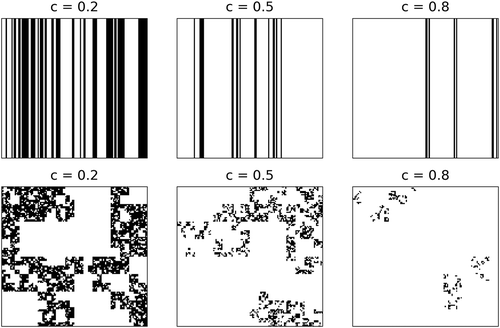
As a consequence of Equation (3)(3) ${\epsilon }_n={\epsilon }_0{\prod }_{i=0}^n\mu {\epsilon }_i$(3) , ${\epsilon }_n$ has only two possible values, either 0 or ${\lambda }_n^c$. c is the characteristic parameter of the model and is equal to the fractal co-dimension of the geometrical field made of the “alive” portion of the generated field. Figure 1 shows some simulations in 1D and 2D, with various c values to give the reader an intuitive feeling of the physical meaning of c. One can note the visible square structures, notably in 2D. This feature is not realistic and is a limitation of this model. This is due to the discrete nature of its underlying construction scheme (see Schmitt 2014 for a continuous version of the β-model). Conservation of the average activity is ensured since${\lambda }_n^c$. It should be noted that this conservation is true only on average, i.e. for numerous realizations, and not for individual ones.

Figure 1. Examples in one dimension (up) or two dimensions (bottom) of fields generated through the implementation of a β-model with various c

2.3 The conditional β-model

In this sub-section, the conditional β-model, which is at the core of this paper, is introduced. The developed process is illustrated in Fig. 2, which will be used for pedagogical purposes, while the text description is generic. More precisely, we start with a field at a given resolution made of zeros (in white), ones (in black), and missing/unknown data (in gold). The goal is to simulate realistic values for the missing portion of the field, while ensuring that the final field has the desired statistical properties; i.e. that it exhibits a fractal behaviour with the correct fractal dimension.

Figure 2. Illustration with a simple case of the successive steps of the conditional β-model. Ones are represented in black, zeros in white, and unknown/missing values in gold. (a) Start of the process: some data is missing and all the underlying increments of the process are unknown. (b) Filling the ones: all the increments needed to retrieve the ones of the original field are set to one. (c) Filling the zeros: a limited number of increments ensuring the zeros of the original field are retrieved are set to zero. (d) The remaining unknown increments are randomly drawn by using the probability distribution of Equation (5)(5) $Pr\left(\mu \epsilon ={\lambda }_1^c\right)={\lambda }_1^{-c}$(5) . More details (including the edge colour highlights can be found in the text

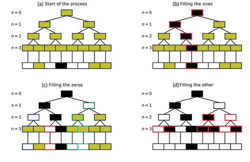
To achieve this, we suggest using a conditioned version of the previously introduced β-model. The assumption is that the field is generated through a multiplicative cascade process, as described in section 2.1. This means that the final field is actually fully defined by all the multiplicative increments of its underlying cascade process (Fig. 2(a)). For a series of length 2ⁿ, the increments to be filled can be denoted $\mu {\epsilon }_{k,i}$, where k is the cascade step ranging from 0 to n and i ranges from 1 to 2^k. They are displayed in gold in Fig. 2(a), since at the beginning of the process they are unknown. Hence, the whole concept of the conditional β-model simply consists in affecting a value to each of the cascade’s multiplicative increments, enabling the reproduction of both the available values and the statistical features. This is what is called conditioning a β-model in this paper.

The general idea of the process presented in this paper is actually rather similar to the process discussed by Tchiguirinskaia et al. (2004). It basically consists in first setting “manually” the increments needed to ensure that the available values are correctly retrieved (i.e. the first level of conditioning of the β-model). In a second step, the remaining increments are simply stochastically drawn using the laws of Equation (5)(5) $Pr\left(\mu \epsilon ={\lambda }_1^c\right)={\lambda }_1^{-c}$(5) , with a parameter c yielding to the wanted fractal dimension (i.e. the second level of conditioning of the β-model). In Tchiguirinskaia et al. (2004), it is done with continuous universal multifractals (Schertzer and Lovejoy 1987), meaning that it is not the increments but the generator that needs to be set. This might be seen as adding complexity, while enabling the handling of nonbinary fields. However, the process does not ensure that the exact values at the available locations are retrieved, but only approximations. The process is stochastic, meaning that the output is not a deterministic field, but an ensemble of realistic realizations.

More precisely, the three successive steps of the process are detailed with the illustrations in Fig. 2:

• First, the required alive increments are filled, i.e. for each strictly positive value of the field, the chain of increments (one per cascade step) leading to this value is all set to one (i.e. “alive”). In the example of Fig. 2, there is only one non-null available value, and the corresponding increments which then must be set to “alive” are outlined in red in Fig. 2(b).

• Second, the increments that are needed to correctly reproduce the zeros of the initial field are set to zero (i.e. “dead”). Given that it is a multiplicative process and that a single zero in the increments chain leading to a final value is sufficient to have it equal zero, the process is slightly more elaborate than for the “alive” values. In practice, each zero of the initial field is treated one after another. The order is randomly chosen (in practice, a random permutation between their positioning indexes is run and they are treated in the obtained order). Then, for a given zero, the chain of increments leading to it is considered. If there are no zeros, then a single increment among the available ones (there might already be some “alive” increments in the chain, and they should not be changed) is set to zero (“dead”) and the others are left unknown. Remember that, given Equation (3)(3) ${\epsilon }_n={\epsilon }_0{\prod }_{i=0}^n\mu {\epsilon }_i$(3) , a single zero is sufficient to ensure that the final value (i.e. the product of the multiplicative increments) will be equal to zero. Hence, there is no need to set more than one of the increments to zero. The increment set to zero is randomly chosen from among the available ones (in practice, a random permutation between their defining position indexes is run and the first element is selected). If there is already a zero in the chain of increments, then nothing is done. This is illustrated in Fig. 2(c). In this example, the first zero treated is the one outlined in red, with its corresponding increment at cascade step 3 set to zero (the ones of cascade step 0, 1 and 2 were already set to one and could not be altered). Then it was the green one (increment at cascade step 1 is set to zero and the ones at cascade step 2 and 3 are left unknown) followed by the dark blue one (increment at cascade step 2 is set to zero while the one at step 3 is left unknown). The last one is the light blue one. For this time step, since a zero was already in its increments’ chain, no additional zero was added. This process limits the number of increments set to zero while ensuring that available values are correctly retrieved.

• Third, all the increments that are not yet filled are randomly drawn by using the probabilities distribution of Equation (5)(5) $Pr\left(\mu \epsilon ={\lambda }_1^c\right)={\lambda }_1^{-c}$(5) . Once a value has been affected to all the increments, it is straightforward to generate a realization of the field (see Fig. 2(d) for an illustration). See section 3.3 if the parameter c is unknown.

3 Results and discussion with numerical simulations

3.1 Individual fields

In this section, the results obtained with individual fields are discussed. This is done through an example shown in Fig. 3. The initial field was generated with the help of a β-model with seven cascade steps (n = 7, leading to series of length 128) and c = 0.2. The field exhibits an excellent fractal behaviour (Fig. 4) with $D_F=0.79$. This value is close to the expected one of 0.8 (=1 − c), and the slight difference is normal given that it is a single realization, and ensemble computations with numerous samples would yield much closer results.

Figure 3. Outputs in one dimension of the conditional β-model for an initial field (top) simulated with c = 0.2. The content for each sub-figure is described through the title above it (more details can be found in the text). With regard to the “partial field” sub-figure, the yellow time steps correspond to the missing data (i.e. the time steps whose content has been artificially removed). With regard to the “Average over realizations” sub-figure, the colour scale goes from 0 (white) to 1 (black) through various levels of grey, and the gold line is simply a representation of the same information as a time series

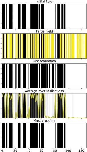
Figure 4. Computation of the fractal dimension (i.e. Equation (2)(2) $N_{\lambda ,A}\approx {\lambda }^{D_F}$(2) in log-log) of the initial field displayed in Fig. 3 (top row)

Then, a portion p of the field is set to missing data. In this example we used $p=0.5$ meaning that half of the field is removed. This is done randomly, and here, it turns out that 64 time steps were “removed” and are now considered missing. The partial field, which is the one used as input in the conditional β-model, is displayed in Fig. 3. Ones are in black, zeros in white and missing data in yellow.

The next step is to implement the conditional β-model to simulate possible realizations for the missing data. Since it is a stochastic process, various realizations ($N_{realisation}$) can be generated. Here we used $N_{realisation}=100$. For each realization, a percentage of hits (a hit rate), i.e. a time step correctly guessed, can be computed by comparing the generated values with the initial ones for all the missing data. In this example, we find that the average percentage of hits ($N_{realisation}=100$) over all realizations is 81% (with a standard deviation of approximately 5%). It should be noted that all of the realizations exhibited the same excellent scaling behaviour with similar fractal dimensions ($D_F=0.79\pm 0.01$).

The average value over all realizations is displayed in Fig. 3, in the fourth row, with shades of grey. White and black correspond to 0 and 1, respectively. In addition to improved clarity, the same quantity is plotted as a time series in yellow ranging from 0 to 1. This quantity is actually an empirically computed probability that the time step will be equal to 1, which corresponds to a probability distribution in this binary framework. Depending on the application, the whole information contained in this probability distribution could be used. In the context of this paper, and in order to remain in a binary framework, we suggest using it to extract a “most probable” (mp) field by setting a time step to 1 if this average is greater than 0.5 and 0 otherwise. This rather natural threshold of 0.5 is actually not arbitrarily chosen. Indeed, a sensitivity analysis showed (not displayed here) that it corresponds to the values leading on average over numerous samples to the maximum percentage of hits for this “most probable” field. This is the field shown in the last row of Fig. 3. The percentage of hits computed on this field (${\mathrm{\%}}_{mp}$) is equal to 87 in this example. Similar results are found with other initial fields.

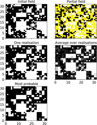
Similar results are found in 2D and illustrated in Fig. 5 for an initial field obtained with five cascade steps and c = 0.2. The same p = 0.5 as before was used and yielded in this case 49% of missing data. $D_F$ on the initial field is equal to 1.81 here with an excellent scaling behaviour. On this example we find ${\mathrm{\%}}_{avg}=79$ and ${\mathrm{\%}}_{mp}=85$.

Figure 5. Outputs in two dimensions of the conditional β-model for an initial field simulated with c = 0.2

3.2 Influence of the various parameters

In this section, the sensitivity of the results to the parameters c of the β-model and p is investigated. To achieve this, the same process as that described in the previous section is implemented on 200 samples of initial fields for each set of parameters (c, p). Results are presented for simulations in 1D, but similar ones are obtained in 2D.

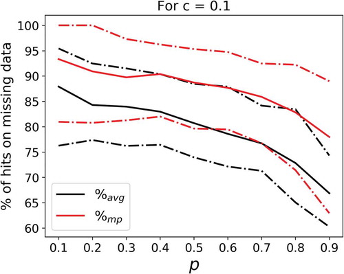
Figure 6 shows the percentage of hits on missing data (called the “hit rate” hereafter) as a function of p for c = 0.1. Black lines are for the average over realizations while red lines are for the “most probable” fields (see the previous section). The uncertainties retrieved over the 200 initial samples are represented as follows: the solid line is the 50% quantile, and the dashed ones are the 10% and 90% quantiles. As expected, the percentage of hits decreases with increasing values of p, and it is now quantified. The performance in terms of scores appears to be 5–10% better with the “most probable” approach, confirming its relevance. Similar results are found for all values of c. Finally, it should be noted that the width of the uncertainty interval is rather large (typically 15–20%), meaning that there is a significant variability of the results from one sample of the initial field to another.

Figure 6. Percentage of hits on the missing data as a function of the proportion p of missing time steps inserted in the initial one-dimensional series for c = 0.1. Black lines indicate the average over realizations while red ones show the most probable fields. Solid lines show the 50% quantile over the 200 samples of initial fields while the dashed lines correspond to the 10 and 90% quantiles

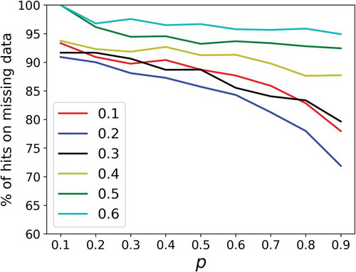
Figure 7 displays the percentage of hits on missing data as function of p for various values of c. To maintain a readable graph, only the 50% quantile over the 200 samples of initial fields with the “most probable” approach is plotted. It corresponds to the red solid line in Fig. 6. The decrease of scores with increasing values of p is found for all c. One can note that even in the worst case, i.e. removing 90% of the initial field with c = 0.2, the percentage of hits remains greater than 70%. Such achievement is possible because the developed model relies on the underlying robust structure of a multiplicative cascade. For a given value of p, there is a tendency for the scores to be better for greater values of c. This suggests that the conditional β-model is better at reproducing the zeros than the ones. This is likely due to the fact that generating an alive time step requires having all the multiplicative increments alive, which turns out to be trickier to obtain. It should be noted that this tendency actually arises only after a sufficient number of cascade steps is reached (typically n > 6–7).

Figure 7. Percentage of hits on the missing data as a function of the proportion p of missing time steps inserted in the initial one-dimensional series for various values of c. Only the 50% quantile over a set of 200 samples of initial fields through the “most probable” approach are plotted (solid red line in Fig. 6)

3.3 How to proceed when c is unknown?

A tricky point is how to proceed when the parameter c of the β-model is unknown. In the previous section, c was always assumed to be known. In situations where this is not the case, we suggest implementing the following algorithm, where $c_{algo}$ is the parameter c used for the simulations:

• Step 1: set $c_{algo}$ to a value. As we will see later, this can be done rather arbitrarily (actually, the output of the algorithm is not sensitive to this initial value), but a natural and simple choice is to set it to $d-D_{F,ini}$ where $D_{F,ini}$ is the fractal dimension of the field assuming the missing data is equal to zero.

• Step 2: compute the “most probable” field using this $c_{algo}$.

• Step 3: estimate the fractal dimension of the retrieved field and update $c_{algo}$ to d minus this fractal dimension.

• Step 4: repeat steps 2 to 4.

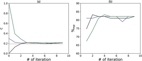
Here are some results obtained in 1D with an initial field generated with $c = 0.2$ and p = 0.7. The fractal co-dimension of the initial field is equal to 0.19. Figure 8 displays the evolution of the parameter $c_{algo}$ as well as ${\mathrm{\%}}_{mp}$ as a function of the number of iterations in the algorithm. For illustrative purposes, the algorithm was run 3 times with three different initial values for $c_{algo}$ (0, 0.3 and 1). Running the algorithms several times with the same initial $c_{algo}$ yields the same results. The first striking feature is that the algorithm rapidly converges towards an asymptotic value of the fractal dimension after only few iterations (Fig. 8(a)). Furthermore, this values does not depend on the initial value of $c_{algo}$. The combination of these two features suggests that the algorithm is robust and can simply be stopped as soon as two successive estimates of c (i.e. the fractal co-dimension of the alive portion of the field) differ by less than 0.05. The final value of c retrieved here is 0.20, which is quite close to the input value of 0.19. Similar results are found for other values of c and p in both 1D and 2D.

Figure 8. Evolution of c and ${\mathrm{\%}}_{mp}$ as a function of the number of iterations in the algorithm to run the conditional β-model when c is unknown. The initial field was generated with c = 0.2 and p = 0.7. The algorithm was started with c equal to 0 (black), 0.3 (blue) and 1 (green)

3.4 Implementation on rainfall data

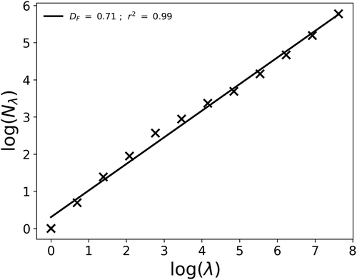
The purpose of this section is to carry out a first implementation of the developed conditional β-model on actual geophysical data. A 5-min rainfall time series of length equal to 2048 time steps is used. It corresponds to a duration of roughly 7.1 d. The series starts on 2019-06-02 00:00:00 (UTC). The studied time series is displayed in Fig. 9. The data was collected on the roof of the Carnot-Cassini building of the École des Ponts ParisTech campus near Paris using an OTT Parsivel² disdrometer (Battaglia et al. 2010, OTT 2014). It is part of the TARANIS observatory of the Fresnel Platform of École des Ponts ParisTech (https://hmco.enpc.fr/portfolio-archive/fresnel-platform/). Interested readers are referred to Gires et al. (2018), who present in details the available database with some data samples for a similar measurement campaign. The total cumulative depth of the series is 29 mm. It contains 323 rainy time steps, i.e. $\approx$16%. Its occurrence pattern, i.e. the geometrical set corresponding to the rainy time steps, exhibits an excellent scaling behaviour with a fractal dimension of 0.71 (see Fig. 10).

Figure 9. Temporal evolution of the rain rate corresponding to the 5 min time step studied rainfall series. Its length is of 2048 time steps, which corresponds to a duration of roughly 7.1 d. The series starts on 2019-06-02 00:00:00 (UTC)

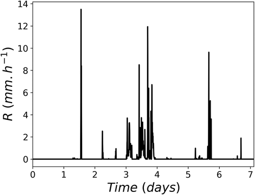
Figure 10. Computation of the fractal dimension (i.e. Equation (2)(2) $N_{\lambda ,A}\approx {\lambda }^{D_F}$(2) in log-log) of the rainfall time series displayed in Fig. 9

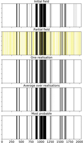
The implementation of the conditional β-model is illustrated in Fig. 11. The 2048-time-step occurrence pattern is displayed at the top of the figure. Below, a partial initial field with approximately half of the time steps set to unknown is shown (obtained with p = 0.5). This means, essentially, that 50% of the recorded data is set aside, and we attempt to reconstruct it with the help of the developed algorithm. Such degraded data was used as input into the algorithm to check its validity. The algorithm was initiated with $c_{algo}$ = 0.1, and two iterations were sufficient to ensure convergence. More precisely, the first iteration yielded a c equal to 0.28, while the second one yielded a value of 0.28 as well, which is also the expected value ($1-D_{F,rainfall}$). Figure 11 displays the outcome after this second iteration of the algorithm: one realization, average, and “most probable” field. The result ${\mathrm{\%}}_{mp}=94$is found, which is very good. Since there are numerous zeros in the field, the hit rate (the percentage of correct hits on missing data) by assuming that all the missing time steps are equal to zero was also computed, and found to be 85%. This highlights the benefits of the conditional β-model. In summary, this first implementation of the conditional β-model on actual data confirms its relevance and efficiency.

Figure 11. Outputs in one dimension of the conditional β-model as in Fig. 3 with an “initial” field consisting of the rainfall time series displayed in Fig. 9

We also tested the threshold of the series before implementing the conditional β-model, i.e. to artificially set to zero all the values below a given threshold T. It turns out that as long as $T<\approx 1$, the resulting field still exhibits good fractal behaviour ($r^2>0.98$ in the computation of $D_F$). The conditional β-model also performs well with ${\mathrm{\%}}_{mp}$ scores for p = 0.5 equal to 97 and 98% for T equal to, respectively, 0.2 and 1 mm.h⁻¹ (the hit rate assuming all missing data is equal to zero is 91% and 95%, respectively). For larger thresholds the quality of the scaling becomes dubious, meaning that the developed approach is no longer relevant. These findings (i) are consistent with the intuitive notion of multifractality, i.e. that a multifractal field consists in a hierarchy of embedded fractal fields; and (ii) confirm that a simple threshold is not appropriate to address this issue and that the notion of singularity, i.e. a kind of scale-invariant threshold, would be required. This would result in a qualitative shift, which is outside the scope of this paper. Some elements in this direction can be found in Tchiguirinskaia et al. (2004).

4 Infilling missing data of imperviousness

4.1 Presentation of the model and the studied catchment

The model and case study are identical to those used by Gires et al. (2018), so only the main elements are summarized here.

The hydrodynamic model used is Multi-Hydro, which was developed at École des Ponts ParisTech (El-Tabach et al. 2009, Giangola-Murzyn et al. 2012, Ichiba et al. 2018). It is a fully distributed, physically based, scalable model that basically consists in an iterative core between widely validated existing models, each of them representing a portion of the water cycle in an urban environment.

In this paper, only the surface and drainage model are used. The surface model is based on the Two-dimensional Runoff, Erosion and eXport model (TREX, Velleux et al. 2011), which models surface flow through a diffusive wave approximation of 2D Saint-Venant equations, and infiltration through a simplification of the Green and Ampt equation. The drainage model is based on the Storm Water Management Model (SWMM), developed by the US Environmental Agency (Rossman 2010), which models flow in the sewer network through a numerical solution of 1D Saint-Venant equations. See Ichiba et al. (2018) and references therein for examples of implementations.

Multi-Hydro requires the rasterization of available geographical information system (GIS) data into a regular grid with a fixed pixel size. For the determination of the unique land-use class for a given pixel, a priority order based on the hydrological importance is used. A pixel’s land-use class will be the one of the class with the highest priority level it contains, regardless of its surfacic significance. The order used here is: gully (because the two-way interactions between surface and drainage flow is handled through these pixels), road, house, forest, grass. This is not the only possible approach to rasterize, and a comparison with one based on surface significance can be found in Ichiba et al. (2018).

The catchment studied in this paper is a 3.017 km² semi-urban area located in Jouy-en-Josas (Yvelines County, southwest of Paris). It is mainly on the left bank of the Bièvre River, which flows general from west to east in the south of the catchment. There is a rather steep slope in the middle of the catchment, with an altitude difference of roughly 100 m between the north of the catchment and its outlet (southeast). More details on the catchment and its flooding history can be found in Gires et al. (2018).

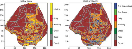
Figures 12(a) and 13(a) display a representation of the studied catchment, with pixels of 2 m and 10 m, respectively. The pixels in yellow correspond to data not available, which were simply filled with “grass” in Gires et al. (2018). They represent 16.2% of the 2 m pixels and 5.6% of the 10 m pixels. As can be seen in Figs 12(a) and 13(a), they are primarily located within the urbanized portion of the catchment around the buildings, meaning that they may typically correspond to small gardens attached to individual houses or private driveways/parking lots. Such areas were not identified on the available GIS data (BD ORTHO, professionnels.ign.fr). This suggests that the automatic treatment performed to obtain the data from the available areal photographs does not allow distinguishing this type of area at the required resolution. Improving the treatment of such pictures to refine the data could be a relevant approach, but it is another field of expertise. Here, the implementation of the conditional β-model will enable us to distinguish in a simplified binary way whether these pixels are pervious or impervious, and hence whether they behave in a very different manner hydrologically speaking.

Figure 12. Representation of the Jouy-en-Josas catchment in Multi-Hydro with 2 m pixels. (a) “Initial” data, hence with missing data. (b) “Most probable” field, where missing data has been replaced by either grass or an impervious area using the developed conditional β-model

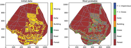
Figure 13. Same as in Fig. 12 size 10 m

4.2 Results and discussion on filling the gaps with the conditional β-model

In this section, we implement the conditional β-model on the land-use representation of the Jouy-en-Josas catchment. More precisely, two classes of pixels are distinguished in order to retrieve the binary framework of the previous sections: impervious pixels (i.e. the pixels corresponding to gully, road and building), and pervious ones (i.e. forest and grass).

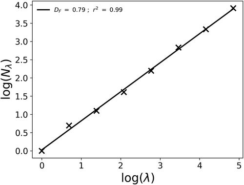
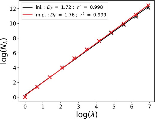
The geometrical set consisting of the impervious area of this catchment was found to exhibit an excellent scaling behaviour, with a fractal dimension of $\approx$1.7 (see Fig. 14 for a computation in an area of 1024 × 1024 pixels) (Gires et al. 2017, p. 2018). Such fractal behaviour suggests that it is possible to use the developed conditional β-model to fill the missing data.

Figure 14. Computation of the fractal dimension (i.e. Equation (2)(2) $N_{\lambda ,A}\approx {\lambda }^{D_F}$(2) in log-log) of the geometrical set made of the impervious areas of the studied catchment with 2 m pixels (i.e. the field displayed in Fig. 12)

For technical reasons, the β-model requires us to work with square fields whose size is equal to a power of two, since in the discrete cascade model, each structure is divided into two sub-structures which enables us to maximize the number of cascade steps for a given final size. In practice, here, the field is embedded in a larger one matching the requirement, which slightly increases computation costs. The added pixels are considered missing. After the conditional β-model has been run, they are simply removed and all the output analysis is carried out on the initial field. In order to limit possible bias associated with the addition of large areas with missing data, the fractal dimensions in the conditional β-model are computed only on the portion corresponding to the initial area.

Figures 12(b) and 13(b) display a representation of the studied catchment with pixels of size 2 m and 10 m respectively, with missing data filled using the “most probable” approach. The missing data found to be impervious (“alive” in the β-model) is shown in blue, while that found to be pervious (“dead” in the β-model) is shown in green (considered to be grass). As might be expected, given the lower initial amount of impervious pixels at 2 m and the priority rule set, a greater portion of pervious areas was generated at 2 m. The quality of the scaling behaviour is slightly improved with this most probable field ($r^2$ goes from 0.998 to 0.999), and the fractal dimension estimate is slightly increased as well, from 1.72 to 1.76 (Fig. 14).

The current version of the hydro-dynamic model only enables a limited number of land-use classes. Hence, we chose to use the binary output of the conditional β-model in the form of the “most probable” field. However, in terms of perspectives, with models having a different approach to represent land-use distribution, the actual probability distribution of the output for a given pixel could be used. For example, it could mean using the average output over numerous realizations to define a given level of imperviousness for each pixel, rather than the binary approach presented here. The purpose of this is simply to illustrate the other possibilities of the developed conditional β-model. Their actual implementation should be carried out in further investigations.

4.3 Results and discussion on the hydrological consequences

Hydrodynamic simulations were then carried out with the help of the Multi-Hydro model with pixels of size 10 m. The initial land-use field with missing data taken as grass, along with the 100 realizations of realistic ways of filling the 5.6% missing data, and the most probable field were used as input. All the other inputs are kept the same. A moderate rainfall event that occurred over roughly 10 h on 9 February 2009, resulting in an average cumulative depth of 9.4 mm over the catchment, is used. Distributed C-band radar rainfall provided by Meteo-France is used. This event was already studied in Gires et al. (2018) and is presented in more detail there.

As in Gires et al. (2018), a pseudocoefficient of variation $CV{ }_{95}^{\prime }$ is used to quantify the variability within the 100 realizations of the generated ensemble (here, of land-use distribution). For a given quantity, it consists in taking half of the difference between the 5% and 95% quantiles divided by the 50% quantile (median) over the 100 realizations:

(6) $CV{ }_{95}^{\prime }=\frac{1}{2}\frac{Q_{95\mathrm{\%}}-Q_{5\mathrm{\%}}}{Q_{50\mathrm{\%}}}$(6)

where Q is the studied quantity, here peak flow or maximum water depth for a given pixel.

The outcomes of the simulations are shown in Fig. 15. In panel (a), the flow at link #507 is visible. It drains the water from the north of the catchment. A zoom during the peak flow is shown in Fig. 15(b). The relative difference at the time of peak flow between the “initial” field and the “most probable” one is 2%. The uncertainty range is limited and the $CV{ }_{95}^{\prime }$ between the various realizations is only 0.5%. These variations are limited, but given that there was only 5.6% missing data, it was expected. Implementing it with the 2 m representation, for which 16.2% of pixels are missing data, would yield stronger variability.

Figure 15. Outcome of the hydrodynamic simulations carried out with the Multi-Hydro model. “Initial” land-use data with the missing data taken as “grass” is used as input along with the 100 realizations of realistic ways of filling the 5.6% missing data, and the “most probable” field. (a) Simulated flows at link #507. Time is indicated since the beginning of the simulation. (b) Zoom of (a) near the peak flow. (c) Map of the difference in simulated maximum water depth between simulations carried out with the “most probable” field and the “initial” one. (d) Map of the $CV{ }_{95}^{\prime }$ coefficient for the maximum water depth

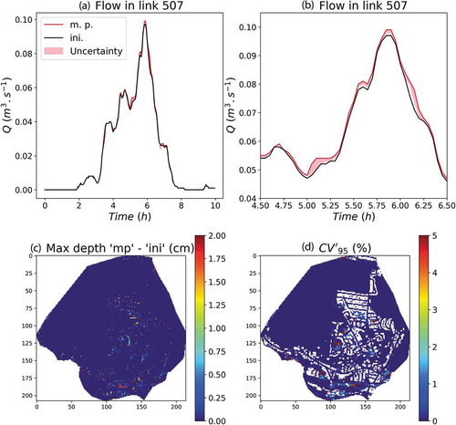
In term of maximum depth for each pixel, the difference between the “most probable” case and the “initial” one is displayed in Fig. 15(c). It reaches 2 cm and is obviously mainly located on the pixels corresponding to missing data. The $CV{ }_{95}^{\prime }$ for this maximum depth is displayed in Fig. 15(d). It can reach more than 5% for some pixels, in areas where more missing data are concentrated.

5 Conclusions and perspectives

In this paper, a conditional version of the β-model is presented. It is designed to fill gaps where there are missing data. The β-model is a binary discrete multiplicative cascade process, meaning that a final field is entirely defined by the multiplicative increments of the underlying cascade. Hence, in the conditional β-model, the multiplicative increments necessary to obtain the desired values at the available locations are set, and then the remaining ones are simply stochastically drawn. As such, an ensemble of possible fields can be obtained, from which a “most probable” field is derived. It corresponds to setting at 1 the portion of the field for which the probability of having a 1 exceeds 0.5. This threshold maximizes the performance of the model. The main advantages of this conditional model with regards to other approaches are: (i) it is physically based in the sense that it preserves and actually relies on underlying scale-invariant properties of the studied geophysical fields; (ii) it can intrinsically work at any resolution; (iii) it requires only one parameter (the fractal dimension of the studied field), thus it is parsimonious; and (iv) it requires limited computational power.

This approach was first tested on numerical simulations, notably to quantify the sensitivity of the conditional β-model to the various parameters, i.e. mainly the fractal dimension of the studied field and the percentage of missing data. When randomly removing up to 90% of a field, the hit rate with this approach when trying to reconstruct the original field is greater than 70%. Such figures can be achieved thanks to the underlying robust structure inherited from the cascade process. The algorithms were then tested on a rainfall occurrence pattern, which enabled a first validation of the developed approach on geophysical data. Finally, the conditional β-model was used to fill the gaps of missing data on imperviousness at high resolution over a 3 km² area near Paris. The ensemble of possible fields was then used as input in an available hydro-dynamic model to quantify the uncertainty associated with these missing data.

In this specific case, due to the available data (only 5% missing data) and resolution used for running the model, the hydrological consequences are limited, with for example less than 2% difference in the peak flow simulated with the various inputs. Such uncertainty in surface and sewer flow is small, and in any case smaller than that associated with other sources of uncertainty such as the spatio-temporal rainfall distribution, or the roughness coefficient variability, for which a single value per land-use type was used. Despite the limited impact, this implementation nevertheless enabled a successful proof of concept of the developed methodology, which was the purpose of this paper. Future work with other case studies, and notably cases where the impact of missing data is more striking (for example, in areas where measurements are sparser) would confirm the usefulness of the developed approach.

In addition, further investigations should compare this conditional β-model with existing methods, such as those discussed in the introduction; and with other geophysical fields. This would likely enable a clearer identification of the model’s advantages and limitations depending on the context.

In this paper, a simple and rather pedagogical conditional model is developed. Yet this conditional β-model is applicable to and has been successfully implemented with rainfall and imperviousness in urban areas. Further investigations should be devoted to shifting from binary fields to full fields and to removing the visible square structures, which would require using continuous multifractal fields.

Acknowledgements

The authors gratefully acknowledge the partial financial support from the Chair of Hydrology for Resilient Cities (endowed by Veolia) of the École des Ponts ParisTech, and the ANR JCJC RW-Turb project (ANR-19-CE05-0022-01).

Disclosure statement

No potential conflict of interest was reported by the authors.

References

- Abudu, S., Bawazir, A.S., and King, J.F., 2010. Infilling missing daily evapotranspiration data using neural networks. Journal of Irrigation and Drainage Engineering, 136 (5), 317–325. doi:10.1061/(ASCE)IR.1943-5464774.0000197.
- Bárdossy, A. and Pegram, G., 2014. Infillling missing precipitation records - a comparison of a new copula-based method with other techniques. Journal of Hydrology, 519, 1162–1170. doi:10.1016/j.jhydrol.2014.08.025.
- Battaglia, A., et al., 2010. PARSIVEL snow observations: a critical assessment. Journal of Atmospheric and Oceanic Technology, 27 (2), 333–344. doi:10.1175/2009JTECHA1332.1.
- Ben Aissia, M.-A., Chebana, F., and Ouarda, T., 2017. Multivariate missing data in hydrology – a review and applications. Advances in Water Resources, 110, 299–309. doi:10.1016/j.advwatres.2017.10.002.
- Coulibaly, P. and Evora, N.D., 2007. Comparison of neural network methods for infilling missing daily weather records. Journal of Hydrology, 341 (1), 27–41. doi:10.1016/j.jhydrol.2007.04.020.
- Dumedah, G. and Coulibaly, P., 2011. Evaluation of statistical methods for infilling missing values in high-resolution soil moisture data. Journal of Hydrology, 400 (1), 95–102. doi:10.1016/j.jhydrol.2011.01.028.
- Dumedah, G., Walker, J.P., and Chik, L., 2014. Assessing artificial neural networks and statistical methods for infilling missing soil moisture records. Journal of Hydrology, 515, 330–344. doi:10.1016/j.jhydrol.2014.04.068.
- El-Tabach, E., et al., 2009. Multi-hydro: a spatially distributed numerical model to assess and manage runoff processes in peri-urban watersheds. In: E. Pascheet, et al., eds. Final Conference of the COST Action C22, Road map towards a flood resilient urban environment. Paris, France: Hamburger Wasserbau-Schriftien.
- Frisch, U., Sulem, P.-L., and Nelkin, M., 1978. A simple dynamical model of intermittent fully developed turbulence. Journal of Fluid Mechanics, 87 (4), 719–736. doi:10.1017/S0022112078001846.
- Garciarena, U. and Santana, R., 2017. An extensive analysis of the interaction between missing data types, imputation methods, and supervised classifiers. Expert Systems with Applications, 89, 52–65. doi:10.1016/j.eswa.2017.07.026.
- Giangola-Murzyn, A. et al., 2012. Multi-component physically based model to assess systemic resilience in Paris Region. In: Proceedings Hydro-Informatics Conference, Hamburg, 14–18 July 2012 Germany.
- Gill, M.K., et al., 2007. Effect of missing data on performance of learning algorithms for hydrologic predictions: implications to an imputation technique. Water Resources Research, 43 (7). doi:10.1029/2006WR005298.
- Gires, A., et al., 2017. Fractal analysis of urban catchments and their representation in semi-distributed models: imperviousness and sewer system. Hydrology and Earth System Sciences, 21 (5), 2361–2375. doi:10.5194/hess-21-2361-2017.
- Gires, A., et al., 2018. Multifractal characterisation of a simulated surface flow: a case study with multi-hydro in Jouy-en-Josas, France. Journal of Hydrology, 558, 483–495. doi:10.1016/j.jhydrol.2018.01.062.
- Gires, A., Tchiguirinskaia, I., and Schertzer, D., 2018. Two months of disdrometer data in the Paris area. Earth System Science Data, 10 (2), 941–950. doi:10.5194/essd-10-941-2018.
- Giustarini, L., et al., 2016. A user-driven case-based reasoning tool for infilling missing values in daily mean river flow records. Environmental Modelling and Software, 82, 308–320. doi:10.1016/j.envsoft.2016.04.013.
- Hentschel, H. and Procaccia, I., 1983. The infinite number of generalized dimensions of fractals and strange attractors. Physica D. Nonlinear Phenomena, 8, 435–444. doi:10.1016/0167-2789(83)90235-X.
- Ichiba, A., et al., 2018. Scale effect challenges in urban hydrology highlighted with a distributed hydrological model. Hydrology Earth Systems Sciences, 22, 331–350. doi:10.5194/hess-22-331-2018.
- Kim, J.-W. and Pachepsky, Y.A., 2010. Reconstructing missing daily precipitation data using regression trees and artificial neural networks for SWAT streamflow simulation. Journal of Hydrology, 394, 305–314. doi:10.1016/j.jhydrol.2010.09.005.
- Lovejoy, S., Schertzer, D., and Tsonis, A.A., 1987. Function box-counting and multiple elliptical dimension in rain. Science, 235, 1036–1038. doi:10.1126/science.235.4792.1036.
- Miró, J.J., Caselles, V., and Estrela, M.J., 2017. Multiple imputation of rainfall missing data in the Iberian Mediterranean context. Atmospheric Research, 197, 313–330. doi:10.1016/j.atmosres.2017.07.016.
- Molnar, P. and Burlando, P., 2005. Preservation of rainfall properties in stochastic disaggregation by a simple random cascade model. Atmospheric Research, 77 (1–4), 137–151. doi:10.1016/j.atmosres.2004.10.024.
- Mwale, F., Adeloye, A., and Rustum, R., 2012. Infilling of missing rainfall and streamflow data in the Shire River basin, Malawi – a self organizing map approach. Physics and Chemistry of the Earth, Parts A/B/C, 50–52, 34–43. doi:10.1016/j.pce.2012.09.006.
- OTT, 2014. Operating instructions, present weather sensor ott parsivel 2. Kempten, Germany: OTT.
- Over, T.M. and Gupta, V.K., 1996. A space-time theory of mesoscale rainfall using random cascades. Journal of Geophysical Research-Atmospheres, 101 (D21), 26319–26331. doi:10.1029/96JD02033.
- Oyler, J.W., et al., 2015. Creating a topoclimatic daily air temperature dataset for the conterminous United States using homogenized station data and remotely sensed land skin temperature. International Journal of Climatology, 35, 2258–2279. doi:10.1002/joc.4127.
- Rossman, L.A., 2010. Storm water management model, user’s manual. Version 5.0. Cincinnati: U.S. Environmental Protection Agency, EPA/600/R–05/040.
- Salvadori, G., Schertzer, D., and Lovejoy, S., 2000. Multifractal objective analysis: conditioning and interpolation. Stochastic Environmental Research and Risk Analysis, 15, 261–283. doi:10.1007/s004770100070.
- Schertzer, D. and Lovejoy, S., 1987. Physical modelling and analysis of rain and clouds by anisotropic scaling and multiplicative processes. Journal of Geophysical Research, 92 (D8), 9693–9714. doi:10.1029/JD092iD08p09693.
- Schertzer, D. and Tchiguirinskaia, I., 2020. A century of turbulent cascades and the emergence of multifractal operators. Earth and Space Science, 7, e2019EA000608. doi:10.1029/2019EA000608.
- Schmitt, F.G., 2014. Continuous multifractal models with zero values: a continuous b-multifractal model. Journal of Statistical Mechanics: Theory and Experiment, 2014. doi:10.1088/1742-5468/2014/02/P02008.
- Sivapragasam, C., et al., 2015. Infilling of rainfall information using genetic programming. Aquatic Procedia, 4, 1016–1022. doi:10.1016/j.aqpro.2015.02.128.
- Tchiguirinskaia, I., et al. 2004. Multiscaling geophysics and sustainable development. Scales in Hydrology and Water Management, IAHS Publ., 287, 113–136.
- Velleux, M.L., England, J.F., and Julien, P.Y., 2011. TREX watershed modelling framework user’s manual: model theory and description. Fort Collins: Department of Civil Engineering, Colorado State University.
- Williams, D.A., et al., 2018. A comparison of data imputation methods using Bayesian compressive sensing and empirical mode decomposition for environmental temperature data. Environmental Modelling and Software, 102, 172–184. doi:10.1016/j.envsoft.2018.01.012.