Application of Granger-causality to study the climate change impacts on depletion patterns of inland water bodies

ABSTRACT

When it comes to projecting the potential effects of climate change on hydro-climatic variables using time-series models, the conventional approach has been to examine correlations with exogenous variables. Establishing correlations among endogenous and exogenous variables, however, cannot guarantee that there is a cause-effect relationship among the variables. This study, therefore, used Granger-causality for a more accurate alternative to the exogenous variables needed to expand time-series models. To demonstrate this, Maharlou Lake, Iran was selected for a case study not only because this inland water body has been exhibiting unprecedented depletion patterns recently, but also because studies are projecting that a changing local climate could add pressure to the region’s water resources. Both restricted and extended models reveal that shrinkage observed in the lake’s time-series data is expected to continue in the near future. This depletion, however, is projected to be more pronounced in August, September, and October, and milder in February, March, and April. Furthermore, the results from the extended model hint at a more severe pattern of shrinkage rooted in the adverse impacts of projected climate change.

KEYWORDS:

• time-series analysis
• shrinking lakes
• climate change
• SARIMA
• augmented Dickey-Fuller test
• Granger-causality

Editor A. Castellarin ; Associate editor H. Tyralis

1 Introduction

Studies have, time and again, proven that human activities are continuously altering the natural world, its dynamics and systems, and its typically consistent patterns, changing the status quo (Gleick 2000). It has become abundantly clear that some of these changes are likely to cause devastating consequences (Huntington 2006, AghaKouchak et al. 2015, Bozorg-Haddad et al. 2020). Perhaps the most notable alteration is anthropogenically driven global warming that is causing climates to change (Alexander et al. 2006, IPCC 2013, Stern and Kaufmann 2014). Experts have cited climate change as a main external driver of the changing patterns of hydro-climatic variables (e.g. Huang et al. 2011, Adhikari et al. 2017, Kazemzadeh and Malekian 2018, Zolghadr-Asli et al. 2019a). These changes may not only manifest in different shapes or forms in each region, but the magnitudes of such alterations may also vary from one region to another (IPCC 2014). Some impacts of shifting patterns of hydro-climate variables are changes in streamflow (e.g. Nijssen et al. 2001), flood hydrographs (e.g. Arora and Boer 2001, Hirabayashi et al. 2013), and magnitudes of droughts (e.g. Stahl et al. 2010). Accordingly, growing evidence supports the projected trends for the foreseeable future (Hakala et al. 2020), and it is clear that water resources will also be affected by such changes (Zolghadr-Asli et al. 2020a).

In the context of hydro-climatology, climate change impacts may cause the shrinkage of inland water bodies, both fresh and saline, including but not limited to lakes (Gao et al. 2011, Wurtsbaugh et al. 2017). From a hydrological standpoint, lakes refer to any body of water, other than an ocean, that is of reasonable size, impounds water, and has little to no horizontal movement of water (Cech 2010). It has been estimated that, in terms of sheer volume, large salt lakes represent 44% of all lakes on Earth (Messager et al. 2016). Unfortunately, many of these lakes are shrinking at alarming rates [e.g. Alemaya and Hora-Kilole Lakes, Ethiopia (Lemma 2003); Dead Seas, West Bank (Yechieli et al. 2006), Ebinur Lake, China (Zhang et al. 2015); Lake Chad, Africa (Coe and Foley 2001); Lake Corangamite, Australia (Timms 2005), Lake Poopó, Bolivia (Zolá and Bengtsson 2006); and Tushka Lakes, Egypt (Bastawesy et al. 2008)]. The degradation of saline lakes is complex, and as such, many factors influence such situations (Khazaei et al. 2019). Nonetheless, there is no denying that climate change either contributed to the creation of the problem (Huang et al. 2011) or has merely amplified it (Khazaei et al. 2019).

Changing climates, in most cases, influence water resources through complex and intricate mechanisms that make it difficult to project the eventual outcomes and the impacts on other systems that rely on them (Hakala et al. 2020, Zolghadr-Asli et al. 2020a). While there are different approaches available to study water bodies such as conceptual hydrological models (e.g. Pulido-Velazquez et al. 2018, Senent-Aparicio et al. 2019) and numeric-oriented techniques (e.g. Jimeno-Sáez et al. 2017), times series modelling are still considered as one of the most popular options available (Zolghadr-Asli et al. 2020b). Time-series analysis and modelling can help capture the underlying relationships between hydro-climate variables and can be used to simulate their behaviours in both absences (e.g. Durdu 2010, Myronidis et al. 2012, Mehdizadeh et al. 2019, Fathian et al. 2019a) and presence (e.g. Fathian 2019, Fathian et al. 2019b) of external stressors. In fact, some have attempted to understand saline lakes’ “behaviours” through this framework (e.g. Myronidis et al. 2012, Mehrian et al. 2016, Fathian 2019, Fathian et al. 2019b). Through modification, these models can replicate the structure of hydro-climatic variables, even when the relationships between the variables are non-linear and non-stationary in nature (Stern and Kaufmann 2014). Non-stationarity, however, can describe a vast set of stochastic behaviours, and the more complicated these patterns are, the more sophisticated are the time-series models needed to mathematically represent these phenomena (Fathian et al. 2019b). Creating hybrid time-series models (e.g. Fathian 2019) or decomposing the time-series to model each component individually (e.g. Zolghadr-Asli et al. 2019b) are commonly used approaches to simplify the said challenge. Nonetheless, when external stressors are included, studying the potential impacts of climate change on water resources, for example, the process of capturing hydro-climate variables’ reactions, becomes even more taxing computationally. The main reason is that it is difficult to objectively quantify or establish cause-effect relationships between external stressors and the behaviour of the time-series data. While statistical measures like correlation can help (Fathian 2019), correlation is not causation. A statistically significant correlation between two variables does not mean that there is a cause-effect relationship between them (Games 1990, Stigler 2005). This fact has been widely neglected in studies of the impacts of external variables on the behaviours of hydro-climatic variables (e.g. Lee et al. 2016, Mehrian et al. 2016, Fathian 2019, Fathian et al. 2019b, Zolghadr-Asli et al. 2020b).

Climate change can have significant impacts on water resources. As such, the status of the water supply is influenced by exogenous variables. The interactions between endogenous and exogenous variables are so complicated that establishing a cause-effect relationship, let alone the magnitude of such impacts, is difficult to the degree that they are often excluded in the development of hydro-climate statistical time-series models. This study explores Granger-causality as a remedy for such complications. In contrast to conventional time-series modelling, which uses correlation to incorporate exogenous variables, Granger-causality can reveal more meaningful and reliable relationships to expand time-series models. In fact, while some studies had implemented the concept of Granger causality to study hydro-climatic variables (e.g. Smirnov and Mokhov 2009, Kodra et al. 2011, McGraw and Barnes 2018), the idea of employing this notion to expand time series models have not been explored yet.

An expanded model can more realistically project the trends of water resources under climate change conditions. In order to demonstrate the use of Granger-causality in the expansion of a statistical time series model, this study focuses on Maharlou Lake, Iran, a once permanent inland water body in south-western Iran that has now reached a critical water level that seasonal drying has turned into a commonly accruing phenomenon (Brisset et al. 2018, Zolghadr-Asli and Behrooz-Koohenjani 2020). The projections of climate change in this region and its influence on water resources (Bozorg-Haddad et al. 2020) make this an ideal example to investigate such relationships as patterns of shrinkage of the lake that are amplified by a changing climate.

2 Materials & methods

Employing Granger-causality to improve the implications of exogenous factors in time-series models will enable projections of future resources that may be affected by changing climates. The two pillars that help shape the methods are statistical time-series modelling and statistical testing (Fig. 1). The former provides a structure to discern the main drivers of hydro-climatic variables. The latter helps shape this structure by determining the most suitable components to use to construct the model.

Figure 1. The flowchart of the modelling procedure

Statistical models capture and represent the time-series data set’s main characteristics using four components: trends, periodicities, autocorrelation, and irregular elements. The trends are the long-run tendencies of the series. Periodicity is the repetitive fluctuation of a time-series variable or set. Among hydro-climatic variables, repetitive patterns often manifest per annum, so they are commonly referred to as seasonal patterns. Autocorrelation is the influence of a lagged step on the “present” state. If autocorrelations of higher-order lags are deemed statistically significant, a time-series is said to have a “long memory”. And irregularity is random and unpredictable elements that bear the stochastic characteristics of white-noise (Adhikari and Agrawal 2013).

The autoregressive moving average (ARMA) is one of the most often used stochastic time-series models (Hipel and McLeod 1994). This class of linear stochastic models is premised on the Markov chain in which previous entries are used to predict the value of the current step. ARMA modelling has often been used to replicate hydro-climatic variables (Fathian et al. 2019b). Most of these variables are naturally not stationary. ARMA models are incapable of handling non-stationary time-series without pre-processing (Araghinejad 2013). Differencing operators can systematically enforce stationarity on time-series data (Ozaki 1977). Using differencing operators (i.e. backshift operators), Box and Jenkins (1970) expanded ARMA models by using a more generalized version of the model, a seasonal autoregressive integrated moving average (SARIMA). The SARIMA(p,d,q)×(P,D,Q)^s model is mathematically expressed as (Adhikari and Agrawal 2013):

(1) ${\mathrm{\Phi }}_P(L^s){\phi }_p(L)(1-L{)}^d(1-L^s{)}^D{y}_t={\mathrm{\Theta }}_Q(L^s){\theta }_q(L){\epsilon }_t$(1)

where y_t = observed value in the tth time step; ε_t = the random error in the tth time step; p = the order of the non-seasonal autoregressive model; d = the order of non-seasonal differencing; q = the order of the non-seasonal moving-average model; P = the order of the seasonal autoregressive model; D = the order of seasonal differencing; Q = the order of the seasonal moving average model; s = the time steps for seasonal differencing; φ and θ = the non-seasonal model parameters for the autoregressive and moving-average models, respectively; Φ and Θ = the seasonal model parameters for the autoregressive and moving-average models, respectively; and L() = backshift operators.

Even though the SARIMA model can capture the stochastic characteristics of a hydro-climatic variable by adjusting orders and tuning model parameters (Box and Jenkins 1973), it is not equipped to identify and replicate the impacts of external stressors. As such, while they can understand the underlying structure of hydro-climatic variables under status quo conditions, these models would struggle to adequately capture the impacts of external variables such as climate change (e.g. Zolghadr-Asli et al. 2020b). In other words, the structure of this model does not account for the impacts of exogenous variables. However, one can use a linear regression-based structure to expand the model to include exogenous variables. The mathematical structure of the expanded model, commonly referred to as a SARIMAX model, is (Araghinejad 2013):

(2) $y_t={\sum }_{i=1}^l{\beta }_i{X}_{t-1}+Z_t$(2)

where β_i = parameter of the transfer function model; X = the vector of exogenous variables; l = the order of exogenous variables; and Z_t = the unexpanded time-series model estimation in the t^th time step.

In the context of hydro-climatic studies, correlation is often used to determine the most important exogenous variables. However, an established correlation may not indicate a cause-effect relationship, so it can be misleading. Technically, exogenous variables influence but are not influenced by endogenous variables. Such relationships, however, cannot be detected by merely exploring the correlation between two variables. One should instead explore and opt for the driving variables.

Granger-causality analyses whether a variable carries unique and useful information that can predict another in a time-series (Granger 1969). As such, a statistically meaningful Granger-caused relation among two variables hints that one’s behaving pattern can be used to improve the prediction of the other variable’s time series. This notion, which in technical terms is referred to as “predictive” causality, however, should not be confused with an “actual” cause-effect relationship, for the latter is mostly a philosophical concept, while the former is a more practical interpretation used to improve the mathematical representation of a phenomenon (Diebold 1998). Though Granger-causality was initially introduced as an economic and financial concept (e.g. Thornton and Batten 1985, Joerding 1986, Hiemstra and Jones 1994), other disciplines are now using it to explore relationships between other subjects (e.g. Chen et al. 2004, Roebroeck et al. 2005, Stern and Kaufmann 2014). To conduct a Granger-causality test, one must find a time-series model that can effectively represent endogenous variables. This provides a base upon which one can add exogenous variables that carry unique and useful pieces of information to improve model performance statistically. Correlation can be used to reduce the number of potentially suitable candidates. Then t-tests can be used to determine whether each variable improves the base model’s performance. F-tests can then be used to evaluate the collective contribution of the selected set of variables. If the results of these tests indicate that an exogenous variable’s contribution was insignificant, the variable can be dropped from the set, and the F-test would be repeated. Unless an exogenous set can pass both the t- and F-tests, that they extend and improve the model’s performance, it is assumed that there is no Granger-causality between exogenous and endogenous variables (Seth 2007).

Through the processes of formation of both the restricted and expanded models, one must assess whether a specific setting can adequately capture the underlying structure of the time-series. The time-series in both formats must be stationary. The augmented Dickey-Fuller test determines whether a dataset contains a unit-root (i.e. non-stationary) (Dickey and Fuller 1981). The null hypothesis of this test is that a unit-root can be seen in the time-series, and it is therefore not stationary. Given that stochastic time-series modelling is premised on stationarity, this test can reveal whether the orders of seasonal and non-seasonal differencing operations sufficiently enforced stationarity in the data sets (Harris 1992). One must also ensure that the residuals of the modelling do not bear significant autocorrelation. The Ljung-Box test detects statically significant autocorrelations in residuals of a time-series model (Ljung and Box 1978). The null hypothesis of this test is that the chronologically ordered data are independently distributed, therefore there is no significant autocorrelation in the time-series. This test determines whether the stochastic time-series models’ seasonal and non-seasonal orders adequately captured the underlying autocorrelation structure of the dataset (Dufour and Roy 1986).

Given the premise and scope of this study, which is to employ local climate change projections as exogenous variables as guidelines to enhance the projections of endogenous variables using statistical time series models, one should obtain the local hydro-climatic projections of a given study area. Here, the climate change projections for this region are obtained using the climate simulations of CanESM2 (Canadian Earth System Model v. 2) under three representative concentration pathways (RCPs), namely RCP 2.6, 4.5, and 8.5, which were then downscaled using the change factor technique. The hydrologic response of the basin was then simulated using the IHACRES models. See Zolghadr-Asli and Behrooz-Koohenjani (2020) for more information on the technical procedure behind these local hydro-climatic projections. The data for the lake’s surface area, which has been monitored via remote sensing in a monthly time-frame, was obtained from Zolghadr-Asli et al. (2020b). It should also be noted that all the computation and statistical analysis in this study took place in Python v.3 environment.

3 Case study

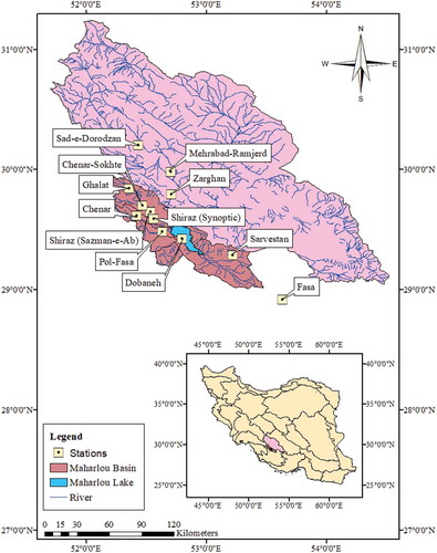
Maharlou Lake (Fig. 2) was considered a permanent inland water body, but, recently, the lake has been experiencing severe and unprecedented fluctuations in the amount of stored water (Brisset et al. 2018). Whereas the lake’s basin, with a catchment area of 4,720 km², has had mild spatial and temporal variations in precipitation, the temperatures have had relatively smaller fluctuations. The average annual precipitation in the southern part of the watershed is approximately 250 mm. In the northern and central portions, however, average annual precipitation is as high as 480 mm. The basin-wide average annual precipitation is approximately 390 mm. Average annual temperatures of the basin, however, range from 18 to 19°C. It should be noted that the said basin can be categorized as a semi-arid to arid region; as such, while temperature shows relatively smaller volatility within annum, as one would expect, precipitation and streamflow show higher inert-annual fluctuations. In fact, all notable stream flows in the region are of seasonal nature. Furthermore, it is worth mentioning that the stream network of the basin is mainly charging the lake, and no notable stream is draining the lake. Recent climate-change projections suggest that there will be a 4% decrease in average annual precipitation, a 0.38°C increase in average annual temperature, and a 24% decrease in average annual streamflow (Zolghadr-Asli and Behrooz-Koohenjani 2020).

Figure 2. The locations of stations in the study area

4 Results & discussion

Although statistical model time series models are reliable choices to understand the underlying structure of hydro-climatic variables under status quo conditions, without additional computational machniasms they are not able to capture the impact of external factors such as the impact of climate change (e.g. Zolghadr-Asli et al. 2020b). As stated, when it comes to projecting the interactions of external stressors and complex inland water bodies such as lakes, conventional statistical time series models, which are popular and efficient ways to capture the underlying structure of hydro-climatic variables, often resort to employing correlations to explore such dynamic relationships between variables. However, this approach cannot adequately do so, given that the presence of statistically significant correlations does not establish the existence of a cause-effect relationship. At the same time, a Granger-causality is an alternative statistical concept that is capable of capturing such relationships. As such, this study aims to promote a framework that is based on this very same premise, and Maharlou Lake has been selected to demonstrate the application of the said approach.

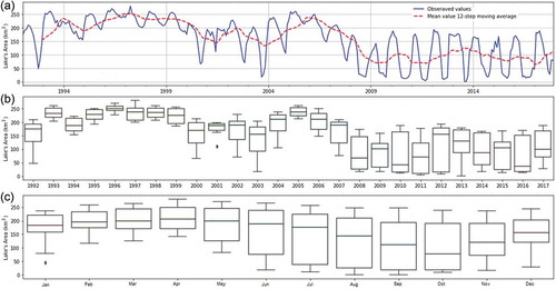
The underlying structure of Maharlou Lake basin’s time-series, monitored during 1992 to 2017, was explored (Fig. 3). The 12-step moving average of the lake’s surface area is revealing a mild downward trend (Fig. 3(a)). A boxplot of the annual observed values also indicates a similar pattern (Fig. 3(b)). A strong seasonal pattern in the data can be seen in a boxplot of monthly observed values (Fig. 3(c)). These visualizations hint that there is non-stationarity in the time-series.

Figure 3. Lake surface area monitored from (1992–2017) as (a) a time-series with a 12-step moving average of the mean and standard deviation; (b) a boxplot of the observed value in each given year; (c) a boxplot of the observed value in each given month

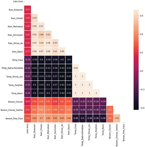
To identify the preliminary set of exogenous hydro-climatic variables that may improve projections of climate-change impacts, three hydro-climatic variables (i.e. rainfall, temperature, and streamflow) were monitored at several locations in the basin and the data were visualized as a heat map (Fig. 4). For each hydro-climatic variable, the endogenous dependent variable (i.e. lake’s surface area) depicts stronger links to individual stations than to the averages of each variable. Therefore, the initial set of exogenous variables were focused on data from individual stations rather than the behavior of the regional averages. As one might expect, though there is a positive correlation among rainfall, streamflow and surface area, temperature is negatively correlated to it. As for the magnitudes of these correlations, streamflow has the strongest relationship to surface area, and precipitation has the weakest. The Ghalat (rainfall), Sad-e-Dorodzan (temperature), and Pol-Fasa (streamflow) stations were selected as the best sources for the initial set of measures of the exogenous variables.

Figure 4. The correlation heatmap plot of the relationships between endogenous and exogenous variables

A restricted time-series model by spitting the dataset into two mutually exclusive sets for training and testing the model. The training set included the data from 1992 to 2012, and the testing includeed the data from 2013 to 2017. A grid-search was used to tune and calibrate the most suitable SARIMA(p,d,q)×(P,D,Q)¹² model for the restricted representation of the lake’s surface area. The orders of the seasonal and non-seasonal differencing ranged from 0 to 1. The orders of seasonal and non-seasonal autoregressive and moving average components ranged between 0 to 3. The grid search then explored > 324 combinations of settings for the model. The augmented Dickey-Fuller tested each setting to determine whether it could satisfactorily reflect the stationarity condition. Two hundred and forty of the settings were found to be feasible for stationarity. Both in-sample (Akaike information criterion (AIC) and Bayesian information criterion (BIC)) and out-sample (root mean square errors (RMSE) and Nash-Sutcliffe efficiency coefficient (NSEC)) measures were used to evaluate and select the best settings for the model. Although the selection criteria (i.e. AIC, BIC, RMSE, and NSEC) helped to identify the better performing settings, they were not able to identify the best setting combination as some of the alternative settings demonstrated slightly better performances based on one criterion, but were outperformed when using other criteria. Therefore, an objective-based multi-attribute decision-making platform, Shannon’s entropy, was used to rank models based on overall performance. Consequently, SARIMA(1,1,2)×(1,1,2)¹² was determined to be the best model to use to represent Maharlou Lake’s surface area (Table 1). The Ljung-Box test, performed on the residual set, indicated that at a 95% confidence level, there were no significant autocorrelation components remained in the residual dataset. Thus the selected model adequately captures the underlying autocorrelation structure of the lake’s surface area time-series.

Table 1. The parameter setting of the selected SARIMA model

The non-seasonal part (d = 1)		The seasonal part (D = 1)
Autoregrressive model (p = 1)	φ1 = 0.85	Autoregrressive model (P = 1)	Φ1 = −0.64
Moving average model (q = 2)	θ1 = −0.79; θ2 = −0.21	Moving average model (Q = 2)	Θ1 = 0.00; Θ1 = −0.50

The individual contributions of the exogenous set’s members were measured by recalibrating the model using different lag periods for each member of the set against the surface area. Based on t-tests, the variables that made significant contributions to the model’s performance were analyzed further (Table 2). As an exogenous variable, temperature made no significant contribution to improving the model’s performance. But three lags (i.e. lags 0, 10, and 11) of streamflow time-series data provided significant, unique information that improved the model’s performance. Lag 10 of rainfall data was also identified as a potentially useful exogenous variable. It is worth noting that the selected lags (i.e. 0, 10, 11, and 12) hint at the potential presence of a short-time seasonal and non-seasonal memory in the structure of the data.

Table 2. The list of potential exogenous variables for expanding the time series model

Hydro-climate variable	Order of lag
Rainfall	10
Temperature	-
Streamflow	0, 10, and 11

The reported values deemed significant at α = 0.05.

To establish Granger-causality among the endogenous and exogenous variables, one must account for the collective impact of the exogenous set on the model’s performance. An iterative testing platform used the F-test to examine the collective impact of exogenous variables. If they did not have significant influences on the model’s performance, the exogenous variables with the least individual influence would be dropped from the set, and the process would be repeated. This algorithm revealed that lag 0 of the streamflow variable (95% confidence) was the only member of the initial exogenous set to convey unique and useful information to strengthen the model. It is worth noting that streamflow is a variable that essentially integrates information about temperature and precipitation, so it was not unexpected when it was revealed that it had a Grander-causality relationship with the endogenous variable. As such, the said variable was added to expand the time-series model. The full model was then implemented to project climate-change impacts on the lake’s surface area.

Three climate-change scenarios, RCP 2.6, RCP 4.5, and RCP 8.5 (Zolghadr-Asli and Behrooz-Koohenjani 2020) were employed to project the values of the exogenous variable into the near-future. The full model then simulated the lake’s surface area under the projected conditions (Fig. 5). All three scenarios indicate that the lake will shrink.

Figure 5. Fitted model’s in-sample predictions (red) and near-future projections (yellow) (for the period from 2018 to 2021) (a) RCP 2.6; (b) RCP 4.5; and (c) RCP 8.5

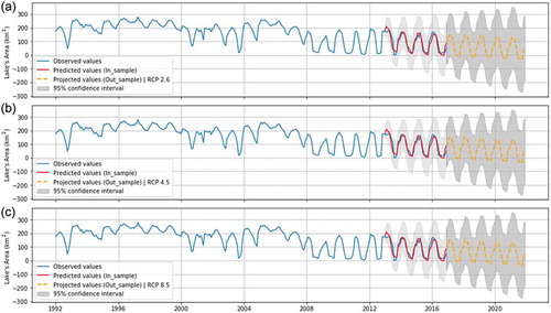
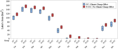
Given that all the extended model’s projections, which are guided by climate change-derived exogenous variable, more or less depict a similar picture they were combined under climate change condition projections. Alternatively, the limited model’s projection, which is not being influenced by any climate change-derived variable, can be labeled as a non-climate change condition projection. Analysis of the projected monthly fluctuations in lake area under both conditions of climate change and no climate change provided further insight into the matter at hand (Fig. 6). While the range of the projected monthly change in surface area widens under climate-change conditions, the overall expected area diminished compared to the no-climate-change effects. Near-future projections indicate that the lake’s expected surface area would drop significantly each month relative to the baseline average monthly observed value. Comparing the restricted to expanded projections, however, shows that climate change is likely to intensify the annual shrinkage of the lake. The relative changes of the average monthly surface area under the projections compared to the baseline data (Table 3) shows that the restricted model, which does not account for climate change, projected that shrinkage would be increased relative to the baseline conditions. Shrinkage would be more pronounced in October (−99%), September (−99%), and August (−96%), and less apparent in February (−23%), March (−26%), and April (−30%). When considering the impact of climate change, −100% reductions of surface area are expected in August, September, and October. The lake would disappear completely during these months. The lake will be smaller in February (−30%), March (−33%), and April (−37%), but is not likely to disappear completely. The expanded model’s projection, which factors in future climate change in the region, predicts higher rates of monthly surface area reduction than does the restricted model’s projection.

Table 3. The relative changes in the lake’s surface area in near future projections in comparison to the baseline condition

	Jan	Feb	Mar	Apr	May	Jun	Jul	Aug	Sep	Oct	Nov	Dec
NCC	−34%	−23%	−26%	−30%	−40%	−65%	−92%	−96%	−99%	−99%	−48%	−44%
CC	−43%	−30%	−33%	−37%	−48%	−76%	−99%	−100%	−100%	−100%	−61%	−55%

Figure 6. The boxplot of the near-future projection for the lake’s surface area in each month under climate-change effect and no climate-change effect conditions

5 Conclusions

Climate change is reshaping the patterns of hydro-climatic variables as well as generating modified responses in environmental systems. As such, it is essential that climate change be addressed in modeling by capturing and reflecting the underlying structures of these variables. From a time-series modeling perspective, hydro-climatic variables are exogenous. The conventional approach to incorporate and quantify the impacts of exogenous variables on the patterns of and responses by endogenous variables, has been to measure the correlations between these variables. Correlation, however, does not necessarily indicate cause and effect. Relying on correlations to improve time-series models often yields increasingly inaccurate projections. For more effective expansion of time-series models, Granger-causality can enable selection of the exogenous variables that provide unique and useful, model-strengthing information. To demonstrate this approach, Maharlou Lake, Iran, was used as a case study. It is an inland water body that has been displaying a shrinking surface area. Recent studies have projected that climate change will stress and reduce this region’s water resources. To that end, A restricted time-series model was used to capture the underlying structure of the lake’s behavior. Granger-causality was used to determine the most useful exogenous (i.e. climate-change) variables to strengthen the model. While several of these variables appeared to provide unique and useful information on their own, when they were tested as a set, it was revealed that there is overlapping information embedded among the variables. Only lag 0 streamflow had a significant Granger-causality relationship with the endogenous variable (i.e. surface area). Lag 0 was added to the restricted time-series model. The extended model was used to project the impact of climate change on the lake areal patterns into the near-future. Both the restricted and extended models revealed that the lake will be shrinking. However, depletion would be more pronounced in August, September, and October, and greater, but not to the same extent, in February, March, and April. The results of the extended model hint at more severe shrinking rooted in changing climates in the region.

Disclosure statement

No potential conflict of interest was reported by the author(s).

References

- Adhikari, R. and Agrawal, R.K., 2013. An introductory study on time series modeling and forecasting. Germany: Lambert Academic Publishing.
- Adhikari, U., et al., 2017. Multiscale assessment of the impacts of climate change on water resources in Tanzania. Journal of Hydrologic Engineering, 22 (2), 05016034. doi:https://doi.org/10.1061/(ASCE)HE.1943-5584.0001467.
- AghaKouchak, A., et al., 2015. Water and climate: recognize anthropogenic drought. Nature, 524 (7566), 409. doi:https://doi.org/10.1038/524409a.
- Alexander, L.V., et al., 2006. Global observed changes in daily climate extremes of temperature and precipitation. Journal of Geophysical Research: Atmospheres, 111 (D5). doi:https://doi.org/10.1029/2005JD006290.
- Araghinejad, S., 2013. Data-driven modeling: using MATLAB® in water resources and environmental engineering. Dordrecht, Netherland: Springer International Publishing Agency.
- Arora, V.K. and Boer, G.J., 2001. Effects of simulated climate change on the hydrology of major river basins. Journal of Geophysical Research: Atmospheres, 106 (D4), 3335–3348. doi:https://doi.org/10.1029/2000JD900620.
- Bastawesy, M.A., Khalaf, F.I., and Arafat, S.M., 2008. The use of remote sensing and GIS for the estimation of water loss from Tushka lakes, southwestern desert, Egypt. Journal of African Earth Sciences, 52 (3), 73–80. doi:https://doi.org/10.1016/j.jafrearsci.2008.03.006.
- Box, G.E.P. and Jenkins, G.M., 1970. Time series analysis: forecasting and control. San Francisco, CA: Holden-Day.
- Box, G.E.P. and Jenkins, G.M., 1973. Some comments on a paper by Chatfield and Prothero and on a review by Kendall. Journal of the Royal Statistical Society. Series A (General), 136 (3), 337–352. doi:https://doi.org/10.2307/2344995.
- Bozorg-Haddad, O., et al., 2020. Evaluation of water shortage crisis in the Middle East and possible remedies. Journal of Water Supply: Research and Technology—AQUA, 69 (1), 85–98. doi:https://doi.org/10.2166/aqua.2019.049.
- Brisset, E., et al., 2018. Late Holocene hydrology of Lake Maharlou, southwest Iran, inferred from high-resolution sedimentological and geochemical analyses. Journal of Paleolimnology, 61 (1), 1–18.
- Cech, T.V., 2010. Principles of water resources: history, development, management, and policy. Danvers, USA: John Wiley & Sons Incorporation.
- Chen, Y., et al., 2004. Analyzing multiple non-linear time series with extended Granger causality. Physics Letters A, 324 (1), 26–35. doi:https://doi.org/10.1016/j.physleta.2004.02.032.
- Coe, M.T. and Foley, J.A., 2001. Human and natural impacts on the water resources of the Lake Chad basin. Journal of Geophysical Research: Atmospheres, 106 (D4), 3349–3356. doi:https://doi.org/10.1029/2000JD900587.
- Dickey, D.A. and Fuller, W.A., 1981. Likelihood ratio statistics for autoregressive time series with a unit root. Econometrica: Journal of the Econometric Society, 49 (4), 1057–1072. doi:https://doi.org/10.2307/1912517.
- Diebold, F.X., 1998. Elements of forecasting. OH, USA: South-Western College Pub.
- Dufour, J.M. and Roy, R., 1986. Generalized portmanteau statistics and tests of randomness. Communications in Statistics-Theory & Methods, 15 (10), 2953–2972. doi:https://doi.org/10.1080/03610928608829288.
- Durdu, Ö.F., 2010. Application of linear stochastic models for drought forecasting in the Büyük Menderes river basin, western Turkey. Stochastic Environmental Research and Risk Assessment, 24 (8), 1145–1162. doi:https://doi.org/10.1007/s00477-010-0366-3.
- Fathian, F., 2019. Dynamic memory of Urmia Lake water-level fluctuations in hydroclimatic variables. Theoretical and Applied Climatology, 138 (1–2), 591–603. doi:https://doi.org/10.1007/s00704-019-02844-6.
- Fathian, F., et al., 2019a. Modeling streamflow time series using non-linear SETAR-GARCH models. Journal of Hydrology, 573, 82–97. doi:https://doi.org/10.1016/j.jhydrol.2019.03.072
- Fathian, F., et al., 2019b. Multiple streamflow time series modeling using VAR–MGARCH approach. Stochastic Environmental Research and Risk Assessment, 33 (2), 407–425. doi:https://doi.org/10.1007/s00477-019-01651-9.
- Games, P.A., 1990. Correlation and causation: a logical snafu. The Journal of Experimental Education, 58 (3), 239–246. doi:https://doi.org/10.1080/00220973.1990.10806538.
- Gao, H., et al., 2011. On the causes of the shrinking of Lake Chad. Environmental Research Letters, 6 (3), 034021. doi:https://doi.org/10.1088/1748-9326/6/3/034021.
- Gleick, P.H., 2000. A look at twenty-first century water resources development. Water International, 25 (1), 127–138. doi:https://doi.org/10.1080/02508060008686804.
- Granger, C.W., 1969. Investigating causal relations by econometric models and cross-spectral methods. Econometrica: Journal of the Econometric Society, 37 (3), 424–438. doi:https://doi.org/10.2307/1912791.
- Hakala, K., et al., 2020. Hydrological modeling of climate change impacts. In: Encyclopedia of water: science, technology, and society. doi:https://doi.org/10.1002/9781119300762.wsts0062.
- Harris, R.I., 1992. Testing for unit roots using the augmented Dickey-Fuller test: some issues relating to the size, power and the lag structure of the test. Economics Letters, 38 (4), 381–386. doi:https://doi.org/10.1016/0165-1765(92)90022-Q.
- Hiemstra, C. and Jones, J.D., 1994. Testing for linear and non-linear Granger causality in the stock price‐volume relation. The Journal of Finance, 49 (5), 1639–1664.
- Hipel, K.W. and McLeod, A.I., 1994. Time series modelling of water resources and environmental systems. Amsterdam, Netherland: Elsevier.
- Hirabayashi, Y., et al., 2013. Global flood risk under climate change. Nature Climate Change, 3 (9), 816–821. doi:https://doi.org/10.1038/nclimate1911.
- Huang, L., et al., 2011. Changing inland lakes responding to climate warming in Northeastern Tibetan Plateau. Climatic Change, 109 (3–4), 479–502. doi:https://doi.org/10.1007/s10584-011-0032-x.
- Huntington, T.G., 2006. Evidence for intensification of the global water cycle: review and synthesis. Journal of Hydrology, 319 (1–4), 83–95. doi:https://doi.org/10.1016/j.jhydrol.2005.07.003.
- IPCC, 2013. Climate change 2013: the physical science basis. Contribution of Working Group I to the Fifth Assessment Report of the Intergovernmental Panel on Climate Change. Cambridge, UK and New York, NY: Cambridge University Press.
- IPCC, 2014. Climate change 2014: impacts, adaptation, and vulnerability. Contribution of Working Group II to the Fifth Assessment Report of the Intergovernmental Panel on Climate Change. Cambridge, UK and New York, NY: Cambridge University Press.
- Jimeno-Sáez, P., et al., 2017. Estimation of instantaneous peak flow using machine-learning models and empirical formula in peninsular Spain. Water, 9 (5), 347. doi:https://doi.org/10.3390/w9050347.
- Joerding, W., 1986. Economic growth and defense spending: Granger causality. Journal of Development Economics, 21 (1), 35–40. doi:https://doi.org/10.1016/0304-3878(86)90037-4.
- Kazemzadeh, M. and Malekian, A., 2018. Changeability evaluation of hydro-climate variables in Western Caspian Sea region, Iran. Environmental Earth Sciences, 77 (4), 120. doi:https://doi.org/10.1007/s12665-018-7305-x.
- Khazaei, B., et al., 2019. Climatic or regionally induced by humans? Tracing hydro-climatic and land-use changes to better understand the Lake Urmia tragedy. Journal of Hydrology, 569, 203–217. doi:https://doi.org/10.1016/j.jhydrol.2018.12.004
- Kodra, E., Chatterjee, S., and Ganguly, A.R., 2011. Exploring Granger causality between global average observed time series of carbon dioxide and temperature. Theoretical and Applied Climatology, 104 (3), 325–335. doi:https://doi.org/10.1007/s00704-010-0342-3.
- Lee, D.E., et al., 2016. Multilevel vector autoregressive prediction of sea surface temperature in the north tropical Atlantic Ocean and the Caribbean Sea. Climate Dynamics, 47 (1–2), 95–106. doi:https://doi.org/10.1007/s00382-015-2825-5.
- Lemma, B., 2003. Ecological changes in two Ethiopian lakes caused by contrasting human intervention. Limnologica, 33 (1), 44–53. doi:https://doi.org/10.1016/S0075-9511(03)80006-3.
- Ljung, G.M. and Box, G.E., 1978. On a measure of lack of fit in time series models. Biometrika, 65 (2), 297–303. doi:https://doi.org/10.1093/biomet/65.2.297.
- McGraw, M.C. and Barnes, E.A., 2018. Memory matters: a case for Granger causality in climate variability studies. Journal of Climate, 31 (8), 3289–3300. doi:https://doi.org/10.1175/JCLI-D-17-0334.1.
- Mehdizadeh, S., et al., 2019. Comparative assessment of time series and artificial intelligence models to estimate monthly streamflow: a local and external data analysis approach. Journal of Hydrology, 579, 124225. doi:https://doi.org/10.1016/j.jhydrol.2019.124225
- Mehrian, M.R., et al., 2016. Investigating the causality of changes in the landscape pattern of Lake Urmia basin, Iran using remote sensing and time series analysis. Environmental Monitoring and Assessment, 188 (8), 462. doi:https://doi.org/10.1007/s10661-016-5456-3.
- Messager, M.L., et al., 2016. Estimating the volume and age of water stored in global lakes using a geo-statistical approach. Nature Communications, 7, 13603. doi:https://doi.org/10.1038/ncomms13603
- Myronidis, D., et al., 2012. An integration of statistics temporal methods to track the effect of drought in a shallow Mediterranean Lake. Water Resources Management, 26 (15), 4587–4605. doi:https://doi.org/10.1007/s11269-012-0169-z.
- Nijssen, B., et al., 2001. Hydrologic sensitivity of global rivers to climate change. Climatic Change, 50 (1–2), 143–175. doi:https://doi.org/10.1023/A:1010616428763.
- Ozaki, T., 1977. On the order determination of ARIMA models. Journal of the Royal Statistical Society: Series C (Applied Statistics), 26 (3), 290–301.
- Pulido-Velazquez, D., et al., 2018. Integrated assessment of future potential global change scenarios and their hydrological impacts in coastal aquifers–a new tool to analyse management alternatives in the Plana Oropesa-Torreblanca aquifer. Hydrology and Earth System Sciences, 22 (5), 3053–3074. doi:https://doi.org/10.5194/hess-22-3053-2018.
- Roebroeck, A., Formisano, E., and Goebel, R., 2005. Mapping directed influence over the brain using Granger causality and fMRI. Neuroimage, 25 (1), 230–242. doi:https://doi.org/10.1016/j.neuroimage.2004.11.017.
- Senent-Aparicio, J., et al., 2019. Coupling machine-learning techniques with SWAT model for instantaneous peak flow prediction. Biosystems Engineering, 177, 67–77. doi:https://doi.org/10.1016/j.biosystemseng.2018.04.022
- Seth, A., 2007. Granger causality. Scholarpedia, 2 (7), 1667. doi:https://doi.org/10.4249/scholarpedia.1667.
- Smirnov, D.A. and Mokhov, I.I., 2009. From Granger causality to long-term causality: application to climatic data. Physical Review E, 80 (1), 016208. doi:https://doi.org/10.1103/PhysRevE.80.016208.
- Stahl, K., et al., 2010. Streamflow trends in Europe: evidence from a dataset of near-natural catchments. Hydrology and Earth System Sciences, 14, 2367–2382. doi:https://doi.org/10.5194/hess-14-2367-2010
- Stern, D.I. and Kaufmann, R.K., 2014. Anthropogenic and natural causes of climate change. Climatic Change, 122 (1–2), 257–269. doi:https://doi.org/10.1007/s10584-013-1007-x.
- Stigler, S.M., 2005. Correlation and causation: a comment. Perspectives in Biology and Medicine, 48 (1), 88–S94. doi:https://doi.org/10.1353/pbm.2005.0045.
- Thornton, D.L. and Batten, D.S., 1985. Lag-length selection and tests of Granger causality between money and income. Journal of Money, Credit and Banking, 17 (2), 164–178. doi:https://doi.org/10.2307/1992331.
- Timms, B.V., 2005. Salt lakes in Australia: present problems and prognosis for the future. Hydrobiologia, 552 (1), 1–15. doi:https://doi.org/10.1007/s10750-005-1501-x.
- Wurtsbaugh, W.A., et al., 2017. Decline of the world’s saline lakes. Nature Geoscience, 10 (11), 816. doi:https://doi.org/10.1038/ngeo3052.
- Yechieli, Y., et al., 2006. Sinkhole ‘swarms’ along the Dead Sea coast: reflection of disturbance of lake and adjacent groundwater systems. Geological Society of America Bulletin, 118 (9–10), 1075–1087. doi:https://doi.org/10.1130/B25880.1.
- Zhang, F., et al., 2015. The influence of natural and human factors in the shrinking of the Ebinur Lake, Xinjiang, China, during the 1972–2013 period. Environmental Monitoring and Assessment, 187 (1), 4128. doi:https://doi.org/10.1007/s10661-014-4128-4.
- Zolá, R.P. and Bengtsson, L., 2006. Long-term and extreme water level variations of the shallow Lake Poopó, Bolivia. Hydrological Sciences Journal, 51 (1), 98–114. doi:https://doi.org/10.1623/hysj.51.1.98.
- Zolghadr-Asli, B. and Behrooz-Koohenjani, S., 2020. Adverse impacts of climate change in Maharlou Lake Basin, Iran. Hydro Science & Marine Engineering. doi:https://doi.org/10.30564/hsme.v2i1.1507.
- Zolghadr-Asli, B., Bozorg-Haddad, O., and Chu, X., 2019a. Effects of the uncertainties of climate change on the performance of hydropower systems. Journal of Water and Climate Change, 10 (3), 591–609. doi:https://doi.org/10.2166/wcc.2018.120.
- Zolghadr-Asli, B., Bozorg-Haddad, O., and Chu, X., 2020a. Hydropower in climate change. In: Encyclopedia of water: science, technology, & society. Wiley & Sons Publication Inc. doi:https://doi.org/10.1002/9781119300762.wsts0089.
- Zolghadr-Asli, B., et al., 2019b. Investigating the variability of GCMs’ simulations using time series analysis. Journal of Water and Climate Change, 10 (3), 449–463. doi:https://doi.org/10.2166/wcc.2018.099.
- Zolghadr-Asli, B., et al., 2020b. A linear/non-linear hybrid time-series model to investigate the depletion of inland water bodies. Environment, Development and Sustainability. doi:https://doi.org/10.1007/s10668-020-01081-6.