Daily streamflow prediction in ungauged basins: an analysis of common regionalization methods over the African continent

ABSTRACT

Predicting streamflow in ungauged basins is a critical task in many projects. This study investigates the applicability and performance of three common regionalization methods over 314 catchments distributed throughout Africa, using the HMETS hydrological model. This study finds that regionalization methods that work well in other regions of the world also do so in the African catchments, except for multiple linear regression which performs worse than expected. Furthermore, skill-based donor filtering is shown to be problematic in some circumstances, notably when the filter rejects mediocre but still useful donors. This study shows that regionalization performance depends more on the hydrological regime of the ungauged catchment and the capacity of hydrological models to adapt to that regime, rather than on any physiographic or climatological metric. In the context of ungauged basins, this indicates that there is no easy recipe to predict the skill of regionalization methods on any given catchment.

KEYWORDS:

• Africa
• regionalization
• prediction ungauged catchment
• physical similarity
• spatial proximity
• regression-based methods
• hydrological model

Editor A. Fiori Associate editor S. Huang

Introduction

Water resources management requires knowledge of streamflow characteristics, including various flow quantiles, for efficient decision-making. This information allows developing water resources systems for hydropower generation, flood protection, irrigation and agricultural use, among others. However, in some regions across the globe, the flow gauging density is either poor or non-existent (Kapangaziwiri et al. 2012). Historically, hydrologists have used methods to transfer flow information from gauged (i.e. “donor”) to ungauged basins using various methods, typically referred to as “regionalization” methods. A large number of regionalization methods have been proposed in the literature since the “decade on the prediction in ungauged basins” of the International Association of the Hydrological Sciences (IAHS) (Sivapalan et al. 2003). Over the past few years, multiple authors have reviewed progress made during this decade and in the years since, and, as can be gleaned from these reviews, there seems to be no consensus on which methods perform best or how to predict if a regionalization method will perform well on a given ungauged catchment (He et al. 2011, Blöschl et al. 2013, Hrachowitz et al. 2013, Parajka et al. 2013, Razavi and Coulibaly 2013, Guo et al. 2021). However, multiple methods with varying degrees of complexity and overall objectives have been proposed over the years.

One of the most prevalent methods is that of the hydrological model parameter regionalization method, which allows the hydrologist to estimate model parameters at the ungauged site and then drive a hydrological model using observed meteorological data to generate continuous streamflow at the ungauged site, usually on a daily or monthly time step. The alternative is estimating hydrological signatures to identify behavioural characteristics at the ungauged site and then generating simulations that fit the characteristics (Bárdossy 2007, Yadav et al. 2007) or regionalizing flow quantiles directly, if the user only needs these metrics for design purposes (e.g. Shu and Ouarda (2007)).

Africa with a size of over 30 million km², is the second largest continent after Asia, and is home to over 1.2 billion people. Some of the largest rivers in the world are found in Africa (Congo River, Nile River, etc.) and so are the largest deserts (Sahara, Kalahari, etc.). Its extremely variable hydrological and climatological regimes make it difficult to apply regionalization methods over the continent (Kapangaziwiri et al. 2012). Even on smaller scales, regionalization methods have been shown to be limited for highly variable hydrological regimes, such as in contrasting climates of Mexico (Arsenault et al. 2019). Furthermore, only approximately 1200 streamflow gauges are publicly available over all of Africa, many of which having only a few years of data, leading to one of the lowest streamflow-station densities in the world (Schuol et al. 2008). Of course, these stations are not uniformly distributed and are mostly located at the outlets of the larger rivers, meaning that the literature contains studies mostly focused on single catchments or on small clusters of catchments.

Three main regions of Africa have been studied at least partially in terms of regionalization. First, the South African region, with its relatively high station density, has received the most attention. Smakhtin et al. (1997) regionalized daily streamflow characteristics in part of the Eastern Cape of South Africa; Smakhtin and Toulouse (1998) studied the impacts of regionalizing low-flow metrics in over 200 catchments of South Africa; Makungo et al. (2010) applied two models using spatial proximity for estimating daily streamflow at a single catchment in South Africa; Kapangaziwiri et al. (2012) compared model-dependent and model-independent regionalization methods in Southern Africa, with similar uncertainty assessments; Winsemius et al. (2009) proposed a framework to integrate soft and hard hydrological information to calibrate a hydrological model on the large ungauged Luangwa River catchment in Zambia; and Ndzabandzaba and Hughes (2017) used hydrological signatures and behavioural parameters to predict flow in five catchments that flow through Swaziland.

The second most studied region is East Africa, mostly in Ethiopia. Kim and Kaluarachchi (2008) found that regional calibration provided more accurate streamflow estimates on the Upper Blue Nile River compared to the multiple linear regression (MLR) regionalization method; Onyutha and Willems (2015) produced empirical regionalization of amplitude-duration-frequency curves for Lake Victoria Basin, East Africa; Tegegne and Kim (2018) compared four regionalization methods using the SWAT hydrological model over the Lake Tana basin in Ethiopia; and Jillo et al. (2017) estimated the water balance on the Omo-Ghibe River basin in Ethiopia using the HBV hydrological model.

The third area of interest in the literature is the Volta River basin in West Africa and its tributaries. Ibrahim et al. (2015) compared multiple linear regression and a parameter kriging method for three of the Volta subcatchments; and Amisigo et al. (2008) studied the monthly streamflow prediction in twelve Volta sub-catchments. Kittel et al. (2020) recently showed for three catchments (two in central Africa and one in North-Western Africa) that transferring parameter sets from a more similar donor catchment performed better in simulating daily streamflow than using closer donor catchments when regionalizing to an ungauged basin. Algeria has also seen some research performed in the field of regionalization, with Zamoum and Souag-Gamane (2019) using classification techniques (principal component analysis – PCA and self-organizing maps – SOM) to provide a basis to regionalize monthly streamflows to 64 river catchments in Algeria, and showing that SOM performed better than PCA when using the GR2M hydrological model. Their results were very promising for monthly and annual streamflow values.

Finally, Beck et al. (2016) performed a global regionalization study using the HBV hydrological model and they integrated 34 hydrometric stations over Africa, with the nearest donor catchment being >5000 km away, on average. They found that the HBV model using global regionalized parameters fared better in Africa than the simple simulation of the global-scale model.

The performance of regionalization over Africa in its entirety, using all available information, has never been performed before. As it can be seen, previous studies have investigated either small or single-catchment sample sizes, have focused on small regional clusters, or have investigated metrics other than daily streamflow. Furthermore, the recommended approaches do not agree from one study to the next. These studies are thus fragmented and do not paint a clear picture of regionalization at the continental scale for Africa. A research gap exists on whether performing regionalization at the continental scale can provide more useful information in the context of daily streamflow prediction in ungauged basins.

The main objective of this study is to analyse and recommend daily streamflow regionalization methods for catchments in Africa by making use of all available gauged catchments to try and determine the best options for various sub-regions and climates. Secondary objectives include comparing results to those obtained in the literature in terms of geography (i.e. the three regional subsets of the African continent as described above) and in terms of similarity (i.e. with similar climates found around the globe), and evaluating the impact of climatological and hydrological regimes on regionalization method performance.

The paper is organized as follows. Following this introduction, a description of the regionalization methods and implementations will be provided. Then, the study area and data will be described, followed by an overview of the methodology. Finally, results and a discussion will be provided in light of the stated study objectives.

Regionalization methods description

Three main model-dependent regionalization methods can be found in the literature and are the most often compared in the regionalization review papers. They are the multiple linear regression (MLR), physical similarity (PS) and spatial proximity (SP) methods. Details for each of these methods implementation can be found in Arsenault and Brissette (2014), but an overview is given here for the sake of clarity. In all cases, the methods depend on transferring the parameters from a hydrological model calibrated on one or more gauged catchments (i.e. donors) to the ungauged site. This allows the hydrological model to be run and to simulate the streamflows at the ungauged site. The regionalization methods are the methods used to perform the actual transfer of parameters and provide the best hydrograph estimation at the ungauged site.

Multiple linear regression (MLR)

The MLR method is based on the assumption that hydrological model parameters represent physical hydrological processes, and that these processes are linked to catchment descriptors (CDs). Catchment descriptors are indicators of catchment physiography, morphology, lithology, climatology and other possible predictors of streamflow regime. In MLR, hydrological model parameters calibrated on donor catchments are used as predictands of a linear regression model that uses the donor catchment CDs as predictors. Therefore, there exists one linear regression model per hydrological model parameter. The models are then applied on the ungauged basin using its CDs to obtain the estimated ungauged basin parameter set. This parameter set is used to run the hydrological model on the ungauged catchment. This method has been shown to perform well in particular circumstances, notably in semi-arid and flat catchments (Blöschl et al. 2013). However, one major problem with this method is that the parameters are evaluated independently, which can be suboptimal if the model parameters are not independent or if the relationships between the CDs and the model parameters are not linear. He et al. (2011) recommend using as many donor catchments as possible to establish these relationships, which is a challenge in poorly gauged regions such as Africa.

Physical similarity (PS)

In PS, the main advantage is that the donor catchment model parameters are kept as an intact set, rather than estimating parameters one at a time such as in MLR. This is done by classifying donor catchments in terms of similarity to the ungauged site and selecting the most similar catchment(s) to transfer the entire parameter set(s). The similarity index θ is used as a metric to quantify the degree of similarity (Burn and Boorman 1993):

(1) $\theta =\sum _{\mathrm{i}=1}^{\mathrm{k}}\frac{\left|{\mathrm{C}\mathrm{D}}_{\mathrm{i}}^{\mathrm{G}}-{\mathrm{C}\mathrm{D}}_{\mathrm{i}}^{\mathrm{U}}\right|}{\mathrm{\Delta }\mathrm{C}{\mathrm{D}}_{\mathrm{i}}}$(1)

where CD_i represents the CD values vector for the gauged (G) and ungauged sites (U), k is the number of catchment descriptors (seven descriptors are used in this study) and ΔCD_i is the range of values that CD can take from the list of available CDs. This method is used to scale the CD values to the same range to equalize their weights in the similarity calculation. This method is based on the hypothesis that similar catchments will have similar hydrological responses, and that the model parameters reflect the hydrological processes in their parameters and structures. However, Oudin et al. (2010) studied this question in detail and showed that this hypothesis is often not verified. Nonetheless, it is still widely used due to its performance compared to other methods (Parajka et al. 2013). The most similar catchment (i.e. the one with the lowest similarity index) is used as the donor and its parameter set is transferred to the ungauged basin to run the hydrological model.

Spatial proximity (SP)

The SP method is a subset of the PS method in which the only CDs used are the latitude and the longitude of the catchment centroids. This becomes equivalent to the Euclidean distance for ranking purposes and thus the model parameters are transferred not from the most similar (in a hydrological and physiographical sense) but from the nearest in the geographical sense. This method is based on the hypothesis that neighboring catchments often share similar attributes, such as soil composition, land cover, land use, slope, elevation, etc. Therefore, in regions where little information on CDs is known, SP can be an enticing option. Furthermore, some CDs are more difficult to measure (such as soil types and bedrock type/depth), meaning that these variables cannot be used in the PS approach. In such cases, SP can contain more information under the proximity hypothesis than by removing these CDs from the equation entirely.

Multi-donor averaging

For the PS and SP methods, the parameter set of the most similar (or nearest) catchment are transferred to the ungauged catchment allowing to simulate a daily hydrograph. However, it has been systematically shown that repeating the process for the second most similar (or nearest) catchment and then averaging both hydrographs usually produces a hydrograph that is more accurate than any of the two individual hydrographs taken individually (Oudin et al. 2008, Reichl et al. 2009, Zhang and Chiew 2009, Samuel et al. 2011). This multi-donor averaging performance increase has been shown to peak at around five to eight donor catchments, after which the added donors typically start to reduce the skill, possibly due to their increasing distance or dissimilarity (Arsenault and Brissette 2014).

One option that was investigated by Oudin et al. (2008) is the idea of using an inverse-distance weighting (IDW) instead of a simple average, whereby the weights are inversely proportional to their distance (or similarity) to the ungauged catchment. Therefore, a very close (or similar) donor would have a greater weight than a very far (or dissimilar) one, reducing the impacts of adding donors that are too different and allowing for a more robust and simple implementation. This strategy has been successfully implemented in (Zhang and Chiew 2009, Samuel et al. 2011). For this study, due to the highly variable nature of the catchments, it is expected that using IDW will reduce the risk associated with considering donors that are too dissimilar or too far from the ungauged catchment.

Skill-based filtering

In the aforementioned regionalization approaches, donors are gauged catchments that: 1) Have been modelled and calibrated with a hydrological model and 2) are near or similar to the ungauged catchment. However, there is no control over the quality of the data at the donor sites, nor is there any requirement regarding the hydrological model’s ability to simulate the streamflows at the donor site. Therefore, it is quite possible that some poorly modelled catchments become donors and negatively influence the results. To mitigate this, Oudin et al. (2008) implemented a filter on donor catchments, by which any catchments that did not obtain a satisfactory calibration skill were excluded from being donors at all, and could not participate in the elaboration of the linear regression models of MLR. Oudin et al. (2008) used donors that had a calibration Nash-Sutcliffe Efficiency of 0.7 or more. Results showed that using this filter improved the regionalization skill across all catchments, including those catchments that were not considered as donors (i.e. had a lower calibration NSE).

Study area and data

Study area

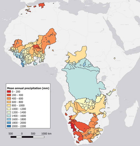
This study was conducted on 314 catchments across all regions of Africa, where catchment boundaries and streamflow gauges of sufficient quality were available, as discussed in the following section. Figure 1 presents the catchment locations and land cover, while Fig. 2 presents the average annual precipitation for each catchment. Table 1 also presents the statistics of the various CDs used in this study.

Table 1. Statistics of the catchment descriptors

Catchment descriptors used in regionalization	Minimum	Maximum	Median	Mean
Mean elevation (m)	32	2550	574	770
Drainage area (km^2)	303	3.65x10^6	6960	64,900
Average slope (%)	0.7	38	3.4	5.5
Land use – Forest (%)	0	98.2	0	4.12
Land cover – Grasslands (%)	0	100	0.32	9.94
Land cover – Savannas (%)	0	100	65.54	54.12
Mean annual precipitation, P (mm)	130	2118	1005	957
Aridity index (P/PET)	0.097	1.268	0.666	0.639
Other catchment properties not used in regionalization	Minimum	Maximum	Median	Mean
Mean annual PET (mm) *	745	1.92x10^3	1.61x10^3	1.49x10^3
Average streamflow, Q (m^3/s) *	0.021	3.98x10^4	16.83	261.3
Runoff ratio (Q/P) *	1.97x10^−4	0.746	0.092	0.129

* PET is used to compute the aridity index but is not used on its own for regionalization. The average streamflow and runoff ratio are for analysis only and not used for regionalization because, by definition, flow and runoff is not available at ungauged sites.

Figure 1. Land cover of Africa with the boundaries of the 314 catchments used in this study. MODIS land cover classes were combined into simpler classes (all types of forest are considered in the “Forest” class), and some minor and insignificant classes (urban, wetlands, snow/ice) were not added to the legend

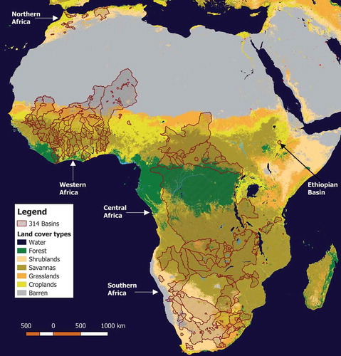
Figure 2. Average annual precipitation for each of the 314 African catchments used in this study. The large spatial variability of precipitation within and across regions can be noted

It can be seen that the selected catchments cover the same regions as those explored individually in previous studies (i.e. the South African region, Volta River basin/West Africa, the Maghreb in Northern Africa and one catchment in Ethiopia/East Africa). There are also some catchments located in Central Africa.

Catchments range in size from 300 km² to over 3 million km², and it can be seen that there are large variations in land cover and precipitation distributions for each of the main regions in the continent. It is also interesting to note that the largest catchment (the Congo River basin corresponding to 13% of the African landmass area) also receives some of the largest precipitation in Africa, which explains why it is the second largest river in the world with average streamflows of almost 40,000 m³/s at the gauging location.

Data

Three types of data were required for this study: (1) climate data to calibrate and drive the hydrological models, (2) observed streamflow data for the hydrological models calibration as well as regionalization performance evaluation, and (3) catchment descriptors derived from multiple geophysical datasets.

Station-based data in Africa is difficult to obtain and generally sparse and of poor quality. Therefore, alternative and well-known data sources were used instead: The ERA5 reanalysis (Hersbach et al. 2020) product for temperature data and the Multi-Source Weighted Ensemble Precipitation (MSWEP; Beck et al. 2017) data for precipitation. Both products cover the period 1981–2018, which were used throughout this study. The ERA5 reanalysis is a gridded near-real-time product that represents the best state of the atmosphere during the assimilation of the European Centre for Medium-Range Weather Forecasts (ECMWF) model. It provides a large set of hydrometeorological variables at the hourly time step and at a ~ 31 km spatial resolution over the entire globe. Previous studies have found that ERA5 climate data is an excellent alternative to station-based data when the weather station network is sparse or of poor quality (Tarek et al. 2020) and was found to be one of the best options for hydrological modelling over Africa (Tarek et al. 2021). MSWEP is a merged multi-source precipitation product that combines gauge, reanalysis and satellite data into a blended product spanning the globe. It was also shown to outperform other precipitation datasets over Africa for hydrological modelling purposes (Tarek et al. 2021). It is available on a 0.25° spatial resolution on a 3-hour time step.

Both ERA5 and MSWEP do not contain any missing data for the entire period and domain. Since there were typically many ERA5 and MSWEP grid points per catchment, all data points located within a given catchment’s boundaries were simply averaged to provide a single time-series for each weather variable. Since this study was performed at the daily scale, the hourly ERA5 data and the 3-hourly MSWEP data were also aggregated by summing precipitation over 24-hour periods coinciding with local time zones, and daily minimum and maximum temperatures were established by taking the minimum and maximum value over the same 24-hour period, respectively.

The hydrometric data was all sourced from the Global Runoff Data Center (GRDC) archive, which contains 9213 stations over all continents, including 1182 over Africa (Do et al. 2017). It is operated by the World Meteorological Organization (WMO) for scientific research purposes. It has been used extensively in the literature as a source of data when hydrometric data is required (Donnelly et al. 2010, Haddeland et al. 2011, Trambauer et al. 2013, Zhao et al. 2017).

Finally, the CDs were computed from the HydroSHEDS (Hydrological data and maps based on the SHuttle Elevation Derivatives at multiple Scales) database (Lehner et al. 2008) and the HydroATLAS database (Linke et al. 2019). HydroSHEDS was used to delineate the catchments at the GRDC gauging stations, and resulting catchment areas were compared to those in the GRDC database. Catchments where GRDC and HydroSHEDS areas were significantly different (i.e. more than 10%) were discarded. Furthermore, a filtering was applied on the catchments to ensure a certain robustness of the regionalization methods. First, only GRDC stations with more than five consecutive years of available data in the (1983–2018) period were kept, to ensure model warm-up and calibration could be performed adequately. Second, all catchments with a surface area less than 300 km² were excluded to eliminate problems related to streamflow timing on sub-daily scales. After the geographic and physiographic processing, 314 catchments across the African continent remained and used in this work (shown in Figs. 1 and Figs. 2).

HydroATLAS provided the other geophysical information data required, namely the physiography data based on the catchment boundaries. Land cover data was sampled from the Moderate Resolution Imaging Spectroradiometer (MODIS) satellite imagery database (Friedl et al. 2002) and grouped by land cover type. Data were catchment-averaged and their statistics are presented in Table 1. Note that some typical indices such as the average streamflow and the runoff ratio are computed and included in Table 1 for information purposes, but they were not used during regionalization as they are not available for ungauged basins, by definition.

Methodology

Hydrological model and calibration

The HMETS (Hydrological Model – École de technologie supérieure; Martel et al. 2017) 21-parameter lumped model has been developed for both research and teaching purposes. While this model has a large number of calibration parameters, 10 of these parameters are used for the snowmelt routine. Considering that none of the study catchments receive any significant snowfall, the model snowmelt routine was removed, substantially simplifying the model. Potential evapotranspiration data are also an input of the HMETS model and is computed using a radiation-based formula developed by Oudin et al. (2005) that has shown to be simple and efficient for rainfall-runoff modelling.

The HMETS model was calibrated using the Kling-Gupta efficiency (KGE; Gupta et al. 2009) metric which aims to provide a multi-objective evaluation based on correlation, variability bias and mean bias. The modified version of the KGE suggested by Kling et al. (2012) is used in this paper and is defined as follows:

(2) $\mathrm{K}\mathrm{G}\mathrm{E}=1-\sqrt{{\left(\mathrm{r}-1\right)}^2+{\left(\alpha -1\right)}^2+{\left(\beta -1\right)}^2}$(2)

where r is the linear correlation coefficient, α is represented by the ratio of the coefficients of variation and β is the ratio of means, all dimensionless statistics computed between the simulated and observed streamflow. The KGE ranges from – ∞ to 1, where 1 indicates a perfect fit and a value of −0.41 indicates that the simulation offers an equivalent performance to the mean streamflow (Knoben et al. 2019). The benchmarks used in this study follows the work of Gutenson et al. (2020) and Pechlivanidis and Arheimer (2015) and are defined as follows: poor (KGE < 0.4), acceptable (0.4 ≤ KGE < 0.7) and good (KGE ≤ 0.7).

The calibration of the HMETS model was done using the CMA-ES (Covariance Matrix Adaptation – Evolution Strategy; Hansen and Ostermeier 1996, 2001) stochastic optimization method. This algorithm has shown to perform better than other methods for hydrological models of larger parameter spaces such as HMETS (Arsenault et al. 2014). The calibration was first performed over all odd years and validation was performed on even years. In all cases, the validation skill was deemed acceptable compared to the calibration skill. Then, as suggested by Arsenault et al. (2018), the calibration was made over all available observations to provide the most optimal results possible. Two calibrations were done for each catchment using the KGE objective function limiting the CMA-ES to a maximum of 15,000 model evaluations, and the best KGE obtained from the two calibrations was kept for the rest of the study.

Regionalization method application and cross-validation

In order to evaluate the regionalization methods’ performance, a typical leave-one-out cross-validation (LOOCV) framework was employed. The implementation is a sequential evaluation of the individual regionalization method’s accuracy to predict streamflow on one of the gauged sites that is considered as ungauged (or pseudo-ungauged) for testing purposes. Each catchment is in turn used as a pseudo-ungauged catchment, and the results of the regionalization over the aggregated set of pseudo-ungauged catchments can be analysed. For each turn, the pseudo-ungauged catchment is not used as a donor, and the model parameters and CDs are not used in establishing the MLR relationships. Therefore, it is considered completely ungauged and can be analysed as such. The hydrographs estimated by regionalization can finally be compared to the actual observed streamflow, and the process is repeated for the next gauged catchment until they have all been the pseudo-ungauged catchment.

All methods are implemented and compared using the LOOCV approach. The MLR, PS and SP are first implemented on their own using a single donor only. Nine CDs were used in defining the similarity metric for PS and to establish the regression models for MLR, which are the eight metrics of Table 1 in addition to the centroid distance between catchments. Then, the PS and SP methods are re-implemented but with increasing numbers of donors. This allows seeing the impact of multi-donor averaging. The IDW averaging implementation was used in this study as previous studies have shown this method to be more robust (as discussed earlier). Then, the skill-based filtering was applied for all methods to evaluate the impact of using a smaller number of high-quality donors instead of a larger set of more varied-quality donors. The skill filtering was performed on the basis of having a calibration KGE > 0.6 and calibration KGE > 0.8 to get a better sense of the impact of calibration skill on regionalization performance. It is important to note that using CDs to characterize similarity has shown limited success in the literature (e.g. Oudin et al. 2010), but can still provide valuable information in data-scarce regions such as the one in this study.

Finally, the regionalization methods were compared by analysing their relative performance at predicting streamflow on the pseudo-ungauged basins and investigating their skill as a function of their size, their relationship with various CDs and their relative distance and similarity to potential donors.

Results

Hydrological model calibration on the donor catchments

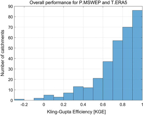
The first step in the methodology was to calibrate all 314 catchments to be used as donors during the regionalization. Figure 3 shows the results of the calibration performance based on the KGE metric for all catchments. Note that most catchments are satisfactorily calibrated, with 250 catchments having KGE values above 0.6 and 156 catchments having KGE values above 0.8. It should be noted that all the KGE values shown are over the calibration period consisting of all available observations. These two thresholds are used in the skill-based filtering tests shown below, as described previously.

Figure 3. Calibration KGE for the 314 catchments. Three catchments have −0.25 < KGE < 0; 30 catchments have 0 < KGE < 0.4; 32 catchments have 0.4 < KGE < 0.6; 96 catchments have 0.6 < KGE < 0.8; and 156 catchments have KGE > 0.8

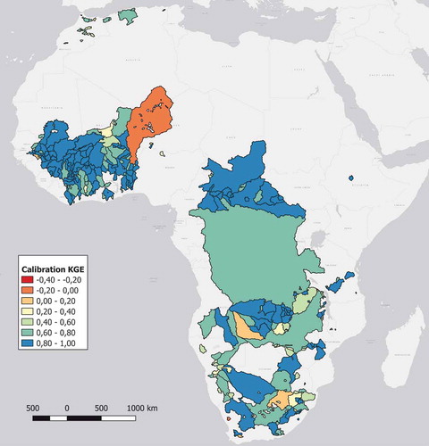
Figure 4 shows the distribution of KGE values over the study area. Smaller catchments are superimposed over the larger ones in the case of nested basins. It can be seen that the larger catchments typically have higher KGE values than the smaller ones, except for the notable case of the Niger River basin (KGE of −0.08 shown in orange) which has a large dried-up section located in the Sahara desert (the Azawagh sub-catchment) which could pose significant challenges to the hydrological model used in this study.

Figure 4. Spatial distribution of the calibration KGE values of the 314 catchments over Africa. Note that the larger catchments typically see better calibration KGE values than smaller catchments, except for the Niger River which is one of the worst in the dataset (KGE of −0.08)

The impact of drainage area on the calibration performance was next investigated. Table 2 shows the average KGE score for the catchments within certain size ranges. It can be seen that there is an increase in average KGE score as the catchment sizes increase.

Table 2. Calibration KGE for different catchment size categories

Size lower bound (km^2)	Size upper bound (km^2)	Number of basins in group	Average calibration KGE score
-	1000	40	0.61
1000	5000	98	0.69
5000	10,000	42	0.77
10,000	100,000	89	0.82
100,000	-	45	0.77*
	Total	314	0.74

* Includes Niger River, with KGE = −0.08. Average becomes 0.79 when Niger River is excluded.

Regionalization method results overview

The next step was to perform the leave-one-out cross-validation (LOOCV) of the three regionalization methods and their variants. Figure 5 shows the results of the SP and PS methods over the 314 pseudo-ungauged catchments while using 1 to 10 donors with the IDW averaging. It can be seen that for both methods, IDW averaging is able to improve the regionalization KGE by adding more than one donor. This gain is more pronounced for the PS method than the SP method. However, it can also be seen that adding more than 4 or 5 donors does not contribute to improving the regionalization performance. This is in line with the findings in the literature for other regions. Since the MLR method does not have any multi-donor (or other) options, its results are shown in each of the panels in Fig. 5 as a comparison measure.

Figure 5. KGE of multiple donor averaging generated hydrographs using the IDW approach for SP (top panel) and PS (bottom panel). Note that improvements plateau at approximately four or five donors for both methods. The x-axis indicates the number of donors that were weighted (Wt1 = one donor, Wt2 = two donors, etc.). The MLR box plot indicates the performance of the MLR method over the study domain and is identical in both panels

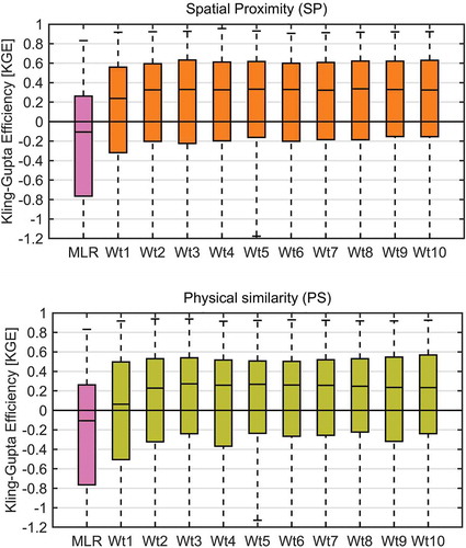
It can be seen from Fig. 5 that the SP method slightly outperforms the PS method, with median KGE values of 0.33 and 0.27, respectively. MLR results are clearly worse, with a negative median KGE value. Figure 6 shows the spatial distribution of the results for each method as well as the comparison of the MLR, PS and SP methods overall, using five donor catchments for PS and SP.

Figure 6. Spatial distribution of the three regionalization methods’ behaviour for the 314 catchments. Each dot’s color represents the ratio between the regionalized (Wt5) and the calibrated (Cal) KGE score for a given pseudo-catchment. The SP and PS regionalization KGE reflects that obtained by using the 5-donor weighted average

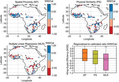
It can be seen in Fig. 6 that the MLR method struggles to obtain positive KGE values, whereas PS and SP show overall more encouraging results. The catchments in the Southern African region are also more distant from one another than those in Western Africa, which could explain the slightly better performance in Western Africa for SP compared to PS. An interesting case is that of the sole Ethiopian catchment, which has a strong calibration KGE (KGE = 0.88) and is located more than 1000 km away from the nearest donor. It is safe to assume, given the variations in land cover between that catchment and its nearest neighbors (see Fig. 1), that the catchments are not close enough for the spatial proximity hypothesis to hold true, i.e. that closer catchments should be more similar and thus should react similarly hydrologically. For this catchment, the PS and MLR methods are able to generate good KGE values (KGE > 0.5), whereas the SP does not perform as well, with KGE < 0.5, as would be expected for a catchment that is far from its donors.

Skill-based filtering

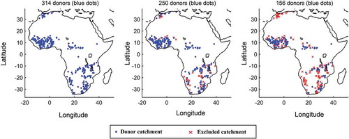
The impact of applying a calibration skill filter was next investigated. Figure 7 shows the spatial distribution of the catchments that are removed after each filtering pass.

Figure 7. Catchments removed from the list of donors following the skill-based filtering. The three panels present the case with all donors (314 donors, left panel), with the KGE > 0.6 filter (250 donors, centre panel) and with the KGE > 0.8 filter (156 donors, right panel). Note that all North Africa and many Southern African catchments are removed with KGE > 0.8

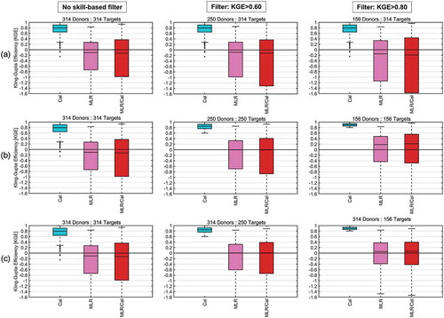
Figures 8–10 respectively show the results for SP, PS and MLR methods. For each of the three regionalization methods, three approaches were tested. First, the regionalization methods used the filtering to remove poorly-calibrated catchments (KGE ≤ filter value) from the donor list, but the regionalization was performed on all sites, including the poorly-calibrated ones (row “A” in Figs. 8–10). The second approach was to remove the poorly-calibrated catchments entirely from the process and to analyse the results of regionalizing only on “well-calibrated” catchments (KGE > filter value) using “well-calibrated” donors (row “B” in Figs. 8–10). Finally, all donors were used to regionalize to only the “well-calibrated” catchments (KGE > filter value) (row “C” in Figs. 8–10). In Figs. 8–10, the left panels represent the base case using all catchments, the centre panels show the results after applying a filter of calibration KGE > 0.6, and the rightmost panels present the results after applying a filter of calibration KGE > 0.8. Therefore, the number of donors reduces from 314 to 250 after the first filter, and from 250 to 156 after the second filter. Results are shown for the calibration, nearest donor, and 5^th nearest donor regionalization KGE for comparison purposes. The results also show the weighted 5-donor KGE values (“Wt5”). The ratio of the 5-donor weighted KGE over the calibration KGE is also presented to contextualize the regionalization skill, since it is not theoretically possible for regionalization to perform better than the calibration.

Figure 8. Spatial proximity (SP) regionalization KGE with skill-based filtering; row (a) regionalizing on all 314 pseudo-ungauged basins, row (b) regionalizing only on the subset of pseudo-ungauged basins that also pass through the filter (regionalizing only on well-calibrated pseudo-ungauged basins), and row (c) using all catchments as donors but regionalizing only on the “well-calibrated” catchments. The left column represents the base case (using all donors on all targets, and all three graphs are therefore identical), the centre column applies the first filter (KGE > 0.60) and the right column applies the second filter (KGE > 0.80). Titles indicate the number of donors and pseudo-ungauged targets used. Each panel has 5 box-plots: “Cal” is the calibration KGE for comparison purposes, “Near_1” is the regionalization KGE using the nearest single donor catchment, “Near_5” is the regionalization KGE using only the 5^th nearest donor catchment, “Wt5” is the weighted 5-donor KGE and “Wt5/Cal” represents the Wt5/Cal ratio to scale the results as a function of the maximum possible attainable skill (i.e. the calibration skill)

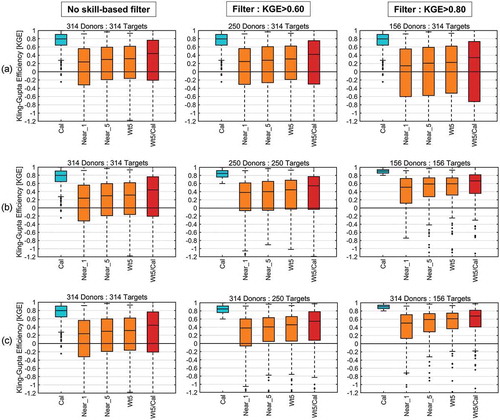
Figure 9. Same as Fig. 8 but for the physical similarity (PS) method

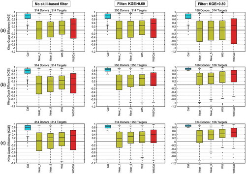
Figure 10. Same as Fig. 8 but for the multiple linear regression (MLR) regionalization method. Each panel presents the calibration KGE, the MLR KGE and the ratio of MLR/Calibration

Results from Fig. 8(a) show that there is practically no difference between regionalizing using all donors and applying a filter of KGE < 0.6 for the SP method. The “Wt5/Cal” ratio even shows a small loss for the bottom quartile of catchments. Surprisingly, applying the second filter (KGE > 0.8) definitely worsens the regionalization skill. Therefore, having “higher-quality”, but fewer donors seems to be detrimental past a certain point. Results from Fig. 8(b) show a different picture: applying the filter to also remove the poorly-calibrated catchments from the regionalization results significantly improves the results. This can be seen in the calibration KGE distribution which progressively increases as the filter removes the poorly-calibrated catchments. The regionalization results follow suit, with net increases after each filter is applied. This points to regionalization method applicability and performance being a function of the hydrological regime and the ability of the hydrological model to model streamflows correctly, rather than other physiographic metrics. Interestingly, using all donors to regionalize to the “well-calibrated” ungauged catchments (Fig. 8(c)) shows similar results to those obtained in (Fig. 8(b)), indicating that most of the improvement comes not from the donors but from the ability of the hydrological model to simulate flows on the target catchments, as evidenced by their high calibration KGE score.

Figure 9 shows the same results as Fig. 8 but for the PS method. Results are somewhat similar, however, the first filter in Fig. 9(a) slightly improves the results. The method still performs slightly worse than the SP method (see Fig. 8(a), centre panel) with this filter. However, the results for the second filter confirm the finding that fewer high-quality donors can be worse than having a larger set of more variable donor catchments. Figure 9(b) shows similar results to those in Fig. 8(b), in that regionalizing on well-calibrated catchments provides better regionalization performance, even after scaling to account for calibration skill. Likewise, regionalizing on only the well-calibrated catchments using all donor catchments performs as well as using only the subset of well-calibrated catchments as donors (Fig. 9(c) vs (Figs. 9b)).

Finally, results for MLR are presented in Fig. 10. For MLR, donors are the catchments that contribute their parameters during the establishment of the parameter-CD relationship. The figure presents the calibration KGE of the target set, the MLR regionalization score and the ratio between both KGE scores.

It can be seen in Fig. 10 that the MLR method’s performance is worse than that of SP (Fig. 8) and PS (Fig. 9) in all cases, both with and without filtering. However, as was the case for SP and PS, the application of the MLR regionalization method on only well-calibrated catchments caused an increase in the regionalization accuracy. Therefore, the MLR method, which is highly dependent on parameter identifiability and relationships with the catchment descriptors, also perform best when applied to catchements whose hydrograph is easier to simulate for the hydrological model. Furthermore, using all donors to establish the MLR regression models only marginally reduces the method’s performance, which further indicates that the regionalization method performance is a function mainly of the target catchment’s ability to be modelled by the hydrological model than by any relationship to CDs or model parameters.

Analysis of predictability of regionalization skill

Finally, the regionalization skill was investigated in light of certain predictors which could potentially be used to predict the regionalization performance on a given ungauged catchment. Table 3 presents the correlation coefficients between the KGE of the MLR, 5-donor SP and 5-donor PS methods and CD values that describe the ungauged catchments.

Table 3. Correlation coefficients between regionalization KGE and the catchment descriptors used in regionalization

	Drainage area	Mean slope	Elevation	Forests	Grass-	Savannas	Ann. Precip.	Aridity
					lands			index
SP_5 Wt	0.01	0.04	−0.08	0.04	0.02	0.07	0.11	0.09
PS_5 Wt	0.03	0.07	−0.08	0.05	−0.01	0.09	0.18	0.18
MLR	0.02	0.02	0.08	−0.13	0.03	0.08	−0.17	−0.15

Table 3 clearly shows that there is no significant correlation between any regionalization method’s performance and values of catchment descriptors. Using them as potential predictors of regionalization skill does not seem to be possible. Similar results were obtained by Kling and Gupta (2009). Other metrics such as the runoff ratio (RR) were also investigated deeper, but yielded very weak correlation with the regionalization skill for any method (not shown).

Discussion

Overview of the regionalization methods’ performance

The overall performance of the regionalization methods used in this study are very similar to those obtained in similar studies across the globe (Oudin et al. 2008, Parajka et al. 2013). SP and PS are still recommended over the MLR method to transfer coherent parameter sets when there are either 1) many parameters used, such as the 11 in this study; or 2) strong links between the parameter values and the CDs, and strong links between the CDs and the hydrological process representation. In this study, MLR performed poorly, which was somewhat expected due to the high levels of parameter interactions in HMETS (Arsenault et al. 2014, Martel et al. 2017).

The multi-donor IDW approach also performed as expected, with regionalization skill improving with the use of two or more donors. Skill seemed to plateau at four or five donors (see Fig. 5), which is also in line with the literature (Oudin et al. 2008, Samuel et al. 2011, Arsenault and Brissette 2014). This is especially important in a hydrologically diverse region such as Africa, due to the higher likelihood of selecting a very different catchment as the first donor. Multi-donor averaging allows mitigating this risk by pooling different simulations and averaging them, typically reducing the errors by averaging them out in the process. It is thus recommended to apply this strategy de facto, especially considering the poor predictability of regionalization method performance in advance.

The SP method also showed slightly better performance than PS in all tests performed in this study. The fact that the catchments were clustered in a few regions also means that the selection of donors is done in the same cluster for SP, whereas for PS the catchments can come from any of the sub-regions. This gives weight to the idea that SP is also a better strategy than PS when a higher density of donor stations is available (Oudin et al. 2008), ultimately selecting more similar neighboring catchments. Furthermore, the incidental test on the isolated Ethiopian catchment (see Fig. 6) showed that it suffered from being distant from its donors and that the MLR and PS methods performed best.

Parajka et al. (2013) performed a meta-analysis of 34 regionalization studies and provided insight on overall regionalization method implementation, predictability and skill depending on catchment attributes and hydroclimatological controls. Here, our study is compared to the meta-analysis of Parajka et al. (2013) to find similarities and differences with the literature. The meta-analysis presents six main points that are applicable worldwide and that we can share comments on:

Regionalization is more accurate in humid than in arid catchments;

Regionalization is more accurate in large than in small catchments;

There is typically a lower performance of regression-based methods (e.g. MLR) compared to SP and PS for studies that compare the three methods;

In humid catchments, SP and PS perform better than regression-based methods;

In arid catchments PS and regression-based methods perform better than SP; and

In regions with dense hydrometric networks, SP’s performance is typically the best.

In this study, the humidity (average precipitation) and aridity index displayed small correlations with regionalization KGE for the PS and MLR methods. SP, which was the most accurate over the entire study on average, had the weakest correlations with the CDs in general. The results also show that regionalization performs best on the catchments that have a higher calibration KGE, and that the larger catchments have a higher calibration KGE, on average. However, the correlation between regionalization KGE and the catchment drainage area is weak (ρ < 0.03). This may be caused by the high variability of catchment drainage areas and the fact that the correlation was performed on all catchments rather than the subset of smaller catchments (point 2). Therefore, although there were arid and humid catchments in this study, the SP method still performed best overall (points 1,4 and 5). We also found that MLR was indeed the worst method in the study when compared to SP and PS, which is in-line with Parajka et al. (2013)’s analysis (point 3). Finally, for point 6, we can state that the SP method performed better than PS in denser regions, as shown in Table 4 below.

Table 4. Average distance (in kilometers) between the ungauged catchment and its nearest donor based on the filtering level for both the SP and PS methods

Filter level	Number of donors left	SP (centroid distance, km)	PS (centroid distance, km)	PS (similarity index, unitless)
No filter	314 donors	140.65	339.11	0.364
KGE > 0.60	250 donors	167.63	371.2	0.398
KGE > 0.80	156 donors	370.55	572.11	0.504

Finally, it is important to recall that there have not been any large-scale regionalization studies over Africa in the literature, even less so at the daily time step. Some studies showed promising results using MLR (e.g. Kim and Kaluarachchi 2008, Ibrahim et al. 2015) but these are at the monthly time step, which makes comparing these studies difficult. The few that have worked on a daily time step show similar results to those in this study, namely in terms of the density of donor stations and data availability (e.g. Makungo et al. 2010). More recently, Kittel et al. (2020) showed that PS performed better than SP on three west African catchments at the daily time step.

Analysis of skill-based filtering

As seen in Figs. 8–10, the skill-based filtering can play a significant role on the regionalization method performance. Oudin et al. (2008) and Arsenault and Brissette (2014) showed that adding a filter increased performance and recommended its application. However, gains were marginal at best for this study for the relatively lax filter. The stricter filter actually reduced performance for all methods. This leads to the finding that the filter can potentially be a good way to exclude poor parameter sets from the process, but removing too many donors also reduces the pool of potential donors, perhaps leading to less similar and more distant donors with an overall negative score. The optimal filter level seems to be case dependent, but it is important to consider in future studies. Table 4 presents an analysis of the impact of donor filtering on the average distance between the ungauged and donor basins. It shows that the first filter (KGE > 0.60) increases the mean distance slightly, but the second filter doubles the average distance for SP and increases the distance from 371 to 572 km for PS. The PS similarity index also increases approximately linearly with the increase in geographical distance.

It is also demonstrated that regionalization methods perform very well on catchments that have high calibration KGE scores and perform poorly on catchments that have poor calibration KGE scores. This indicates that the extent to which an ungauged catchment’s streamflow can be predicted is largely related to the ability of the hydrological model to simulate its hydrological regime, and has less to do with the relationships between catchment descriptors and parameter sets. These findings corroborate those of Knoben et al. (2020) who also found few links between hydrological model performance, the number of model parameters and a large set of hydrological, climatological and physiographic descriptors. Instead, the ability of the hydrological model to simulate the hydrological regime is key, and therefore the same is true in regionalization: the most important variable in regionalization is the model structure and how it is able to represent the ungauged catchment’s streamflow regime. This can be highly affected by the quality of the hydrometric data, as poor-quality streamflow data will de facto cause modelling errors that will pose difficulties for any regionalization method. Therefore, finding a filter level that removes poorly-calibrated catchments from the donor pool without increasing the distance too much could be an approach worth investigating further.

The MLR method is not nearly as affected as PS and SP by the skill-based filter. Reasonably, since MLR uses all available donors to establish the regression models, removing some donors should not drastically influence the established relationships, and thus they are more robust to this filter. However, it is important to recall that even if MLR is more robust to skill-based filtering, it still performs significantly worse than the other two methods.

Limitations

This study was performed using all the data that was publicly available over Africa and for which catchment contours and other physiographic attributes were available. This resulted in a selection of 314 catchments that could be used for the analysis. Many regionalization studies have used more catchments on much smaller domains: Oudin et al. (2008) worked with 913 catchments in France, Patil and Stieglitz (2015) regionalized 756 catchments in the United States, Parajka et al. (2015) performed a similar study by top-kriging interpolation on 555 catchments in Austria and Li and Zhang (2017) used 605 catchments in Australia, for example. The density of catchments is thus much smaller in this study than in previous ones using similar numbers of catchments. It is important to note, however, that the spatial distribution of the 314 catchments in this study is not uniform, but clustered around the humid regions and large river catchments. Regionalization within these clusters is thus more similar to typical regionalization studies. However, the few catchments in North Africa and in Ethiopia in this study do not benefit from this clustering effect, and could be more negatively impacted by the regionalization approaches as was the Ethiopian catchment in Fig. 6. For example, Parajka et al. (2015) found that a station density of at least 2 stations per 1000 km² was a good indicator of strong Nash-Sutcliffe regionalization, whereas densities of less than 1 station per 1000 km² was an indicator of less accurate regionalization efficiency. Oudin et al. (2008), on the other hand, found that SP and PS performed very similarly for station densities of 0.6 stations per 1000 km², and SP gained an increasing edge over PS as the station density increased. This is in line with the findings of this study.

Another limitation is the relatively small scope of this study in terms of methodological choices. For example, a single hydrological model (HMETS) was used instead of repeating the study with two or more models. This would have allowed to better assess the uncertainty related to the choice of a hydrological model, at the expense of more complexity during the results analysis. However, other studies that used more than one hydrological model typically found similar results across models, i.e. the best regionalization method for one model was also the best method for the other models, regardless of the actual evaluation metric score. Furthermore, using more complex models such as distributed and more physically-based models could influence the results and remains to be done in future work. In the same vein, objective function selection for model calibration and regionalization evaluation definitely plays a role on the results. KGE was selected as a good, overall metric; however, if specific objective functions were to be required (e.g. extreme events), the conclusions of this study could be different.

Finally, some of the rivers could be partially regulated, which can influence the streamflow to some extent and cause more modelling problems due to the inability of HMETS to simulate lakes and reservoirs. Since most catchments displayed good calibration and validation KGE scores, it was assumed that any impoundments or water control structures did not play a crucial role in the ability of HMETS to simulate flow in the study area basins.

Conclusion

Predicting streamflow in ungauged catchments has always been an important goal in the hydrological sciences. Numerous methods, and even multiple classes of methods, have been developed to aid in this pursuit. This study compared three hydrological-model based regionalization methods on 314 catchments throughout Africa to compare their performance on a large set of hydrologically diverse catchments and to perform the first large-sample regionalization study on the continent.

This study concludes that, as is the case in most other regions of the world, physical similarity (PS) and spatial proximity (SP) perform better than the multiple linear regression (MLR) approach, due to the transfer of coherent parameter sets rather than parameter sets that are estimated piecewise. The results also show that inverse distance weighting (IDW) of multiple donors still adds value to the regionalization methods, despite the high variability of the catchment climatological and physiographic attributes.

It was also shown that filtering donor catchments based on their calibration skill can have a significant impact on the results, depending on how strict the filter is. Indeed, the results point to the regionalization performance being highly correlated with the ability of the hydrological model to simulate the flows on the ungauged catchment. Therefore, having more information on the type of hydrological regime could help identify appropriate model structures that would allow more accurate regionalization method application.

Taken together, these points paint a clear picture on the applicability of regionalization methods in Africa. It seems clear that, for daily hydrograph regionalization, the following conditions would need to be met:

1. There should be a wide array of donor catchments (ideally a minimum of four or five), ideally located near the ungauged site;

The hydrological model used should be selected carefully to ensure it is able to represent the processes as well as possible (e.g. arid vs humid climates);

SP should be used if the number of nearby catchments is significant, PS should be used otherwise;

Implementing the IDW framework is essential to reduce the risk of selecting a poor donor catchment.

These conditions can be met in multiple regions of Africa (Central, Western and Southern Africa in this study), however, regionalizing in areas which are not currently densely gauged is therefore a riskier proposition that cannot be validated. Testing this directly, however, should be performed in a future study.

Acknowledgements

The authors would like to thank ECMWF for making available the ERA5 reanalysis data and the GRDC for providing the streamflow observation data. We would like to acknowledge the contribution of the creators of the HydroSHEDS and HydroATLAS databases for making this study possible.

ERA5 data are available at: https://cds.climate.copernicus.eu/cdsapp#!/dataset/reanalysis-era5-single-levels?tab=overview

GRDC data are available at: https://www.bafg.de/GRDC/EN/Home/homepage_node.html

HydroSHEDS The HydroSHEDS database and more information are available at http://www.hydrosheds.org.

HydroATLAS data are available at: https://www.hydrosheds.org/page/hydroatlas.

Finally, we extend our thanks to the anonymous reviewers whose comments helped improve the paper and shape it into its current form.

Disclosure statement

No potential conflict of interest was reported by the author(s).

Additional information

Funding

This study has been partly funded by the Egyptian Armed Forces (Ministry of Defense). The Natural Sciences and Engineering Research Council of Canada (NSERC) also partly funded this project through François Brissette and Richard Arsenault’s respective discovery grants [grant nos. RGPIN-2015-05048 and RGPIN-2018-04872].

References

- Amisigo, B.A., et al., 2008. Monthly streamflow prediction in the Volta Basin of West Africa: a SISO NARMAX polynomial modelling. Physics and Chemistry of the Earth, Parts A/B/C, 33 (1), 141–150. doi:https://doi.org/10.1016/j.pce.2007.04.019.
- Arsenault, R., et al., 2014. Comparison of stochastic optimization algorithms in hydrological model calibration. Journal of Hydrologic Engineering, 19 (7), 1374–1384. doi:https://doi.org/10.1061/(ASCE)HE.1943-5584.0000938.
- Arsenault, R., et al., 2019. Streamflow prediction in ungauged basins: analysis of regionalization methods in a hydrologically heterogeneous region of Mexico. Hydrological Sciences Journal, 64 (11), 1297–1311. doi:https://doi.org/10.1080/02626667.2019.1639716.
- Arsenault, R., Brissette, F., and Martel, J.-L., 2018. The hazards of split-sample validation in hydrological model calibration. Journal of Hydrology, 566, 346–362. doi:https://doi.org/10.1016/j.jhydrol.2018.09.027
- Arsenault, R. and Brissette, F.P., 2014. Continuous streamflow prediction in ungauged basins: the effects of equifinality and parameter set selection on uncertainty in regionalization approaches. Water Resources Research, 50 (7), 6135–6153. doi:https://doi.org/10.1002/2013WR014898.
- Bárdossy, A., 2007. Calibration of hydrological model parameters for ungauged catchments. Hydrology and Earth System Sciences Discussions, 11 (2), 703–710. doi:https://doi.org/10.5194/hess-11-703-2007.
- Beck, H.E., et al., 2016. Global-scale regionalization of hydrologic model parameters. Water Resources Research, 52 (5), 3599–3622. doi:https://doi.org/10.1002/2015WR018247.
- Beck, H.E., et al., 2017. MSWEP: 3-hourly 0.25 global gridded precipitation (1979–2015) by merging gauge, satellite, and reanalysis data. Hydrology and Earth System Sciences, 21 (1), 589–615. doi:https://doi.org/10.5194/hess-21-589-2017.
- Blöschl, G., et al., 2013. Runoff prediction in ungauged basins: synthesis across processes, places and scales. New York, United-States: Cambridge University Press.
- Burn, D.H. and Boorman, D.B., 1993. Estimation of hydrological parameters at ungauged catchments. Journal of Hydrology, 143 (3), 429–454. doi:https://doi.org/10.1016/0022-1694(93)90203-L.
- Do, H.X., Westra, S., and Leonard, M., 2017. A global-scale investigation of trends in annual maximum streamflow. Journal of Hydrology, 552, 28–43. doi:https://doi.org/10.1016/j.jhydrol.2017.06.015
- Donnelly, C., et al., 2010. High-resolution, large-scale hydrological modelling tools for Europe. IAHS Publication, 340, 553–561.
- Friedl, M.A., et al., 2002. Global land cover mapping from MODIS: algorithms and early results. Remote Sensing of Environment, 83 (1), 287–302. doi:https://doi.org/10.1016/S0034-4257(02)00078-0.
- Guo, Y., et al., 2021. Regionalization of hydrological modeling for predicting streamflow in ungauged catchments: a comprehensive review. WIREs Water, 8 (1), e1487. doi:https://doi.org/10.1002/wat2.1487.
- Gupta, H.V., et al., 2009. Decomposition of the mean squared error and NSE performance criteria: implications for improving hydrological modelling. Journal of Hydrology, 377 (1), 80–91. doi:https://doi.org/10.1016/j.jhydrol.2009.08.003.
- Gutenson, J.L., et al., 2020. Comparison of generalized non-data-driven lake and reservoir routing models for global-scale hydrologic forecasting of reservoir outflow at diurnal time steps. Hydrology and Earth System Sciences, 25 (5), 2711–2729. doi:https://doi.org/10.5194/hess-24-2711-2020.
- Haddeland, I., et al., 2011. Multimodel estimate of the global terrestrial water balance: setup and first results. Journal of Hydrometeorology, 12 (5), 869–884. doi:https://doi.org/10.1175/2011JHM1324.1.
- Hansen, N. and Ostermeier, A., Adapting arbitrary normal mutation distributions in evolution strategies: the covariance matrix adaptation. In: ed. Proceedings of IEEE International Conference on Evolutionary Computation, 20–22 May 1996 Nagoya, Japan. 312–317.
- Hansen, N. and Ostermeier, A., 2001. Completely derandomized self-adaptation in evolution strategies. Evolutionary Computation, 9 (2), 159–195. doi:https://doi.org/10.1162/106365601750190398.
- He, Y., Bárdossy, A., and Zehe, E., 2011. A review of regionalisation for continuous streamflow simulation. Hydrology and Earth System Sciences, 15 (11), 3539–3553. doi:https://doi.org/10.5194/hess-15-3539-2011.
- Hersbach, H., et al., 2020. The ERA5 global reanalysis. Quarterly Journal of the Royal Meteorological Society, 146 (730), 1999–2049. doi:https://doi.org/10.1002/qj.3803.
- Hrachowitz, M., et al., 2013. A decade of Predictions in Ungauged Basins (PUB)—a review. Hydrological Sciences Journal, 58 (6), 1198–1255. doi:https://doi.org/10.1080/02626667.2013.803183.
- Ibrahim, B., et al., 2015. Hydrological predictions for small ungauged watersheds in the Sudanian zone of the Volta basin in West Africa. Journal of Hydrology: Regional Studies, 4, 386–397.
- Jillo, A.Y., et al., 2017. Characterization of regional variability of seasonal water balance within Omo-Ghibe River Basin, Ethiopia. Hydrological Sciences Journal, 62 (8), 1200–1215. doi:https://doi.org/10.1080/02626667.2017.1313419.
- Kapangaziwiri, E., Hughes, D.A., and Wagener, T., 2012. Incorporating uncertainty in hydrological predictions for gauged and ungauged basins in southern Africa. Hydrological Sciences Journal, 57 (5), 1000–1019. doi:https://doi.org/10.1080/02626667.2012.690881.
- Kim, U. and Kaluarachchi, J.J., 2008. Application of parameter estimation and regionalization methodologies to ungauged basins of the Upper Blue Nile River Basin, Ethiopia. Journal of Hydrology, 362 (1), 39–56. doi:https://doi.org/10.1016/j.jhydrol.2008.08.016.
- Kittel, C.M.M., et al., 2020. Informing hydrological models of poorly gauged river catchments – a parameter regionalization and calibration approach. Journal of Hydrology, 587, 124999. doi:https://doi.org/10.1016/j.jhydrol.2020.124999.
- Kling, H., Fuchs, M., and Paulin, M., 2012. Runoff conditions in the upper Danube basin under an ensemble of climate change scenarios. Journal of Hydrology, 424–425, 264–277. doi:https://doi.org/10.1016/j.jhydrol.2012.01.011
- Kling, H. and Gupta, H., 2009. On the development of regionalization relationships for lumped watershed models: the impact of ignoring sub-basin scale variability. Journal of Hydrology, 373 (3), 337–351. doi:https://doi.org/10.1016/j.jhydrol.2009.04.031.
- Knoben, W.J.M., et al., 2020. A brief analysis of conceptual model structure uncertainty using 36 models and 559 catchments. Water Resources Research, 56 (9), e2019WR025975. doi:https://doi.org/10.1029/2019WR025975.
- Knoben, W.J.M., Freer, J.E., and Woods, R.A., 2019. Technical note: inherent benchmark or not? Comparing Nash–Sutcliffe and Kling–Gupta efficiency scores. Hydrology and Earth System Sciences, 23 (10), 4323–4331. doi:https://doi.org/10.5194/hess-23-4323-2019.
- Lehner, B., Verdin, K., and Jarvis, A., 2008. New global hydrography derived from spaceborne elevation data. Eos, Transactions American Geophysical Union, 89 (10), 93–94. doi:https://doi.org/10.1029/2008EO100001.
- Li, H. and Zhang, Y., 2017. Regionalising rainfall-runoff modelling for predicting daily runoff: comparing gridded spatial proximity and gridded integrated similarity approaches against their lumped counterparts. Journal of Hydrology, 550, 279–293. doi:https://doi.org/10.1016/j.jhydrol.2017.05.015
- Linke, S., et al., 2019. Global hydro-environmental sub-basin and river reach characteristics at high spatial resolution. Scientific Data, 6 (1), 283. doi:https://doi.org/10.1038/s41597-019-0300-6.
- Makungo, R., et al., 2010. Rainfall–runoff modelling approach for ungauged catchments: a case study of Nzhelele River sub-quaternary catchment. Physics and Chemistry of the Earth, Parts A/B/C, 35 (13), 596–607. doi:https://doi.org/10.1016/j.pce.2010.08.001.
- Martel, J.-L., et al., 2017. HMETS—A simple and efficient hydrology model for teaching hydrological modelling, flow forecasting and climate change impacts. International Journal of Engineering Education, 33 (4), 1307–1316.
- Ndzabandzaba, C. and Hughes, D.A., 2017. Regional water resources assessments using an uncertain modelling approach: the example of Swaziland. Journal of Hydrology: Regional Studies, 10, 47–60.
- Onyutha, C. and Willems, P., 2015. Spatial and temporal variability of rainfall in the Nile Basin. Hydrology and Earth System Sciences, 19 (5), 2227–2246. doi:https://doi.org/10.5194/hess-19-2227-2015.
- Oudin, L., et al., 2005. Which potential evapotranspiration input for a lumped rainfall–runoff model?: part 2—Towards a simple and efficient potential evapotranspiration model for rainfall–runoff modelling. Journal of Hydrology, 303 (1), 290–306. doi:https://doi.org/10.1016/j.jhydrol.2004.08.026.
- Oudin, L., et al., 2008. Spatial proximity, physical similarity, regression and ungaged catchments: a comparison of regionalization approaches based on 913 French catchments. Water Resources Research, 44 (3). doi:https://doi.org/10.1029/2007WR006240.
- Oudin, L., et al., 2010. Are seemingly physically similar catchments truly hydrologically similar? Water Resources Research, 46 (11). doi:https://doi.org/10.1029/2009WR008887.
- Parajka, J., et al., 2013. Comparative assessment of predictions in ungauged basins – part 1: runoff-hydrograph studies. Hydrology and Earth System Sciences, 17 (5), 1783–1795. doi:https://doi.org/10.5194/hess-17-1783-2013.
- Parajka, J., et al., 2015. The role of station density for predicting daily runoff by top-kriging interpolation in Austria. Journal of Hydrology and Hydromechanics, 63 (3), 228–234. doi:https://doi.org/10.1515/johh-2015-0024.
- Patil, S.D. and Stieglitz, M., 2015. Comparing spatial and temporal transferability of hydrological model parameters. Journal of Hydrology, 525, 409–417. doi:https://doi.org/10.1016/j.jhydrol.2015.04.003
- Pechlivanidis, I. and Arheimer, B., 2015. Large-scale hydrological modelling by using modified PUB recommendations: the India-HYPE case. Hydrology and Earth System Sciences, 19 (11), 4559–4579. doi:https://doi.org/10.5194/hess-19-4559-2015.
- Razavi, T. and Coulibaly, P., 2013. Streamflow prediction in ungauged basins: review of regionalization methods. Journal of Hydrologic Engineering, 18 (8), 958–975. doi:https://doi.org/10.1061/(ASCE)HE.1943-5584.0000690.
- Reichl, J.P.C., et al., 2009. Optimization of a similarity measure for estimating ungauged streamflow. Water Resources Research, 45 (10). doi:https://doi.org/10.1029/2008WR007248.
- Samuel, J., Coulibaly, P., and Metcalfe, R.A., 2011. Estimation of continuous streamflow in Ontario ungauged basins: comparison of regionalization methods. Journal of Hydrologic Engineering, 16 (5), 447–459. doi:https://doi.org/10.1061/(ASCE)HE.1943-5584.0000338.
- Schuol, J., et al., 2008. Modeling blue and green water availability in Africa. Water Resources Research, 44 (7). doi:https://doi.org/10.1029/2007WR006609.
- Shu, C. and Ouarda, T.B.M.J., 2007. Flood frequency analysis at ungauged sites using artificial neural networks in canonical correlation analysis physiographic space. Water Resources Research, 43 (7). doi:https://doi.org/10.1029/2006WR005142.
- Sivapalan, M., et al., 2003. IAHS Decade on Predictions in Ungauged Basins (PUB), 2003–2012: shaping an exciting future for the hydrological sciences. Hydrological Sciences Journal, 48 (6), 857–880. doi:https://doi.org/10.1623/hysj.48.6.857.51421.
- Smakhtin, V.Y., Hughes, D.A., and Creuse-Naudin, E., 1997. Regionalization of daily flow characteristics in part of the Eastern Cape, South Africa. Hydrological Sciences Journal, 42 (6), 919–936. doi:https://doi.org/10.1080/02626669709492088.
- Smakhtin, V.Y. and Toulouse, M., 1998. Relationships between low-flow characteristics of South African streams. Water SA, 2, 107–112.
- Tarek, M., Brissette, F., and Arsenault, R., 2021. Uncertainty of gridded precipitation and temperature reference datasets in climate change impact studies. Hydrology and Earth System Sciences, 25 (6), 3331–3350. doi:https://doi.org/10.5194/hess-25-3331-2021.
- Tarek, M., Brissette, F.P., and Arsenault, R., 2020. Evaluation of the ERA5 reanalysis as a potential reference dataset for hydrological modelling over North America. Hydrology and Earth System Sciences, 24 (5), 2527–2544. doi:https://doi.org/10.5194/hess-24-2527-2020.
- Tegegne, G. and Kim, Y.-O., 2018. Modelling ungauged catchments using the catchment runoff response similarity. Journal of Hydrology, 564, 452–466. doi:https://doi.org/10.1016/j.jhydrol.2018.07.042
- Trambauer, P., et al., 2013. A review of continental scale hydrological models and their suitability for drought forecasting in (sub-Saharan) Africa. Physics and Chemistry of the Earth, Parts A/B/C, 66, 16–26. doi:https://doi.org/10.1016/j.pce.2013.07.003.
- Winsemius, H.C., et al., 2009. On the calibration of hydrological models in ungauged basins: a framework for integrating hard and soft hydrological information. Water Resources Research, 45 (12). doi:https://doi.org/10.1029/2009WR007706.
- Yadav, M., Wagener, T., and Gupta, H., 2007. Regionalization of constraints on expected watershed response behavior for improved predictions in ungauged basins. Advances in Water Resources, 30 (8), 1756–1774. doi:https://doi.org/10.1016/j.advwatres.2007.01.005.
- Zamoum, S. and Souag-Gamane, D., 2019. Monthly streamflow estimation in ungauged catchments of northern Algeria using regionalization of conceptual model parameters. Arabian Journal of Geosciences, 12 (11), 342. doi:https://doi.org/10.1007/s12517-019-4487-9.
- Zhang, Y. and Chiew, F.H.S., 2009. Relative merits of different methods for runoff predictions in ungauged catchments. Water Resources Research, 45 (7). doi:https://doi.org/10.1029/2008WR007504.
- Zhao, F., et al., 2017. The critical role of the routing scheme in simulating peak river discharge in global hydrological models. Environmental Research Letters, 12 (7), 075003. doi:https://doi.org/10.1088/1748-9326/aa7250.